On the measurement of the proton-air cross section
using cosmic ray data

Abstract

Cosmic ray data may allow the determination of the proton-air cross section at ultra-high energy. For example, the distribution of the first interaction point in air showers reflects the particle production cross section. As it is not possible to observe the point of the first interaction $X_{\rm 1}$ of a cosmic ray primary particle directly, other air shower observables must be linked to $X_{\rm 1}$. This introduces an inherent dependence of the derived cross section on the general understanding and modeling of air showers and, therfore, on the hadronic interaction model used for the Monte Carlo simulation. We quantify the uncertainties arising from the model dependence by varying some characteristic features of high-energy hadron production.

1 Introduction

The natural beam of cosmic ray particles extends to energies far beyond the reach of any earth-based accelerator. Therefore cosmic ray data provides an unique opportunity to study interactions at extreme energies. Unfortunately, the cosmic ray flux is extremely small making direct measurements of the particles and their interactions impossible above $\sim$ 100 TeV. One is forced to rely on indirect measurements such as extensive air shower studies, where interpretation of the data is very difficult.

In this contribution we will briefly discuss different methods of measuring the proton-air cross section, focusing on methods that are based on extensive air shower (EAS) data. Figure 1 shows a compilation of proton-air cross section measurements and predictions of hadronic interaction models currently used in cosmic ray studies [1, 2, 3, 4, 5, 6, 7, 8, 9, 10, 11]

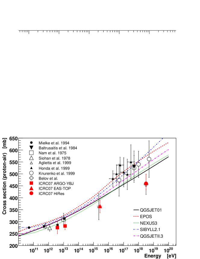
Figure 1: Current data of proton-air production cross section measurements [1, 2, 3, 4, 5, 6, 7, 8, 9, 10, 11] and model predictions [12, 13, 14, 15, 16, 17, 18].

2 Methods of cross section measurements using cosmic ray data

2.1 Primary cosmic ray proton flux

Already in the 60’s first estimates of the proton-air cross section $\sigma_{\rm p-air}$ were made using cosmic ray data [1]. These early measurements are relying on two independent observations of the flux of primary cosmic ray protons after different amounts of traversed atmospheric matter. Firstly the primary proton flux $\Phi(X_{\rm top})$ is measured at the top of the atmosphere with a satellite or at least very high up in the atmosphere on a balloon at $X_{\rm top}=0-5$ gcm^-2. The second flux $\Phi(X_{\rm bottom})$ is measured with a ground based calorimeter at $X_{\rm bottom}=600-1000$ gcm^-2, preferentially at high altitude and using efficient veto detectors to select unaccompanied hadrons. The effective attenuation length can then be calculated straightforwardly from

$$\lambda_{\rm prod}=(X_{\rm bottom}-X_{\rm top})/\log(\Phi_{\rm top}/\Phi_{\rm bottom}).$$ (1)

As it is impossible to veto all hadronic interactions along the cosmic ray passage through the atmosphere, this attenuation length can only be used to obtain a lower bound to the high energy particle production cross section

$$\sigma_{\rm p-air}\geq\frac{\langle m\rangle}{\lambda_{\rm prod}},$$ (2)

where $\langle m\rangle$ is the mean mass of air. The method is limited to proton energies lower than $\sim$TeV, since no sufficiently precise satellite or balloon borne data is available above this energy. By design the unaccompanied hadron flux is only sensitive to the particle production cross section, since primary protons with interactions without particle production cannot be separated from protons without any interaction.

2.2 Extensive air showers

In order to measure $\sigma_{\rm p-air}$ at even higher energies it is necessary to rely on EAS data [6, 7, 8, 9, 10, 11]. The characteristics of the first few extremely high energy hadronic interactions during the startup of an EAS are paramount for the resulting air shower. Therefore it should be possible to relate EAS observations like the shower maximum $X_{\rm max}$, or the total number of electrons $\left.N_{\rm e}(X)\right|_{X=X_{\rm obs}}=N_{\rm e}^{\rm rec}$ and muons $\left.N_{\mu}(X)\right|_{X=X_{\rm obs}}=N_{\mu}^{\rm rec}$ at a certain observation depth $X_{\rm obs}$, to the depth of the first interaction point and the characteristics of the high energy hadronic interactions.
Ground based observations

In case of ground based extensive air shower arrays, the frequency of observing EAS of the same energy at a given stage of their development is used for the cross section measurement. By selecting EAS of the same energy but different directions, the point of the first interaction has to vary with the angle to observe the EAS at the same development stage. The selection of showers of constant energy and stage depends on the particular detector setup, but the typical requirement is $\left(N_{\rm e}^{\rm rec},\;N_{\mu}^{\rm rec}\right)=\rm{const}$ at observation level.

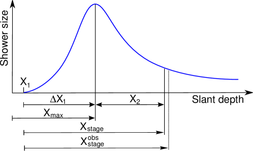
Figure 2: Definition of variables to characterize EAS longitudinal profiles.

With the naming conventions given in Fig. 2, the probability of observing a shower of a given energy $E_{0}$ and shower stage at the zenith angle $\theta$ can be written as

$$\frac{1}{N}\left.\frac{dN}{d\cos\theta}\right|_{N_{\rm e}^{\rm rec},N_{\mu}^{\rm rec}} = \int dX_{1}\int d\Delta X_{1}\int d\Delta X_{2}\;\;\frac{e^{-X_{\rm 1}/\lambda_{\rm int}}}{\lambda_{\rm int}}$$ (3)

$$\times\;P_{1}(\Delta X_{1})\times P_{2}(\Delta X_{2})$$

$$\times\;P_{\rm res}(X^{\rm rec}_{\rm stage},X_{1}+\Delta X_{1}+\Delta X_{2}).$$

Here $X_{\rm stage}$ defines the distance between the first interaction point and the depth at which the shower reaches a given number of muons and electrons as defined by the selection criteria. The experimentally inferred shower stage at observation level $X^{\rm rec}_{\rm stage}$ does, in general, not coincide with the true stage due to the limited detector and shower reconstruction resolution. This effect is accounted for by the factor $P_{\rm res}$. The functions $P_{1}$ and $P_{2}$ describe the shower-to-shower fluctuations. The probability of a shower having its maximum at $X_{\rm max}=X_{1}+\Delta X_{1}$ is expressed by $P_{1}$. The probability $P_{2}$ is defined correspondingly with $X_{\rm stage}=\Delta X_{1}+\Delta X_{2}$.

In cross section analyses, Eq. (3) is approximated by an exponential function of $\sec\theta$. Assuming that the integration of (3) over the distributions $P_{1}$, $P_{2}$, and $P_{\rm res}$ does not yield any generally non-exponential tail at large $\sec\theta$, it can be written as

$$\frac{1}{N}\left.\frac{dN}{d\cos\theta}\right|_{N_{\rm e}^{\rm rec},N_{\mu}^{\rm rec}}\;\propto\;e^{-X_{\rm obs}/\Lambda_{\rm obs}^{\rm S}}\;\propto\;e^{-\sec\theta/\Lambda_{\rm obs}^{\rm S}}.$$ (4)

However, the slope parameter $\Lambda_{\rm obs}^{\rm S}$ does not coincide with the interaction length $\lambda_{\rm int}$ due to non-Gaussian fluctuations and a possible angle-dependent experimental resolution. Therefore the measured attenuation length can be written as

$$\Lambda_{\rm obs}^{\rm S}=\lambda_{\rm int}\cdot k_{\Delta X_{\rm 1}}\cdot k_{\Delta X_{\rm 2}}\cdot k_{\rm resolution}^{\rm S}=\lambda_{\rm int}\cdot k_{\rm S}.$$ (5)

The $k$-factors $k_{\Delta X_{\rm 1}}$, $k_{\Delta X_{\rm 2}}$ and $k_{\rm resolution}^{\rm S}$ parametrize the contributions to $\Lambda_{\rm obs}^{\rm S}$ from the corresponding integrations. However, these integrations are difficult to perform separately and the individual $k$-factors are not known in most analyses (for a partial exception, see [10]).
Observations of the shower maximum $\mathbf{X_{\rm max}}$

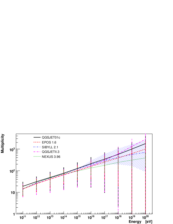
Figure 3: Model predictions for the secondary particle multiplicity in high energy hadronic interactions. The lines denote the mean while the error bars indicate the RMS of the distributions. The shaded area is the range for SIBYLL using $0.3\geq f_{\rm 10EeV}\geq 3$.

Observing the position of the shower maximum directly allows one to simplify (3) by removing the term due to the shower development after the shower maximum $P_{2}$. Also the detector resolution $P_{\rm res}$ is much better under control for $X_{\rm max}$ and can be well approximated by a Gaussian distribution. The resulting distribution is

$$P(X_{\rm max}^{\rm rec}) = \int dX_{\rm 1}\int d\Delta X_{\rm 1}\;\;\frac{e^{-X_{\rm 1}/\lambda_{\rm int}}}{\lambda_{\rm int}}\times\;P_{1}(\Delta X_{1})\times\;P_{res}(X_{\rm max}^{\rm rec}-X_{\rm max}),$$ (6)

with $X_{\rm 1}+\Delta X_{\rm 1}=X_{\rm max}$. In analogy to Eq. (4) only the tail of $P(X_{\rm max}^{\rm rec})$ at large $X_{\rm max}^{\rm rec}$ is approximated by an exponential distribution

$$P(X_{\rm max}^{\rm rec})\;\propto\;e^{-X_{\rm max}^{\rm rec}/\Lambda_{\rm obs}^{\rm X}},$$ (7)

whereas the exponential slope $\Lambda_{\rm obs}$ can be deduced from the convolution integral (6) as

$$\Lambda_{\rm obs}^{\rm X}=\lambda_{\rm int}\cdot k_{\Delta X_{\rm 1}}\cdot k_{\rm resolution}^{\rm X}=\lambda_{\rm int}\cdot k_{\rm X}.$$ (8)

Again $k_{\Delta X_{\rm 1}}$ and $k_{\rm resolution}^{\rm X}$ are the contributions to $\Lambda_{\rm obs}^{\rm X}$ from the corresponding integrations of (6).
It was also recognized that (6) can be unfolded directly to retrieve the original $X_{\rm 1}$-distribution, if the $\Delta X_{\rm 1}$-distribution is previously inferred by Monte-Carlo simulations [11]. Recently this triggered some discussion about the general shape and model dependence of the $\Delta X_{\rm 1}$-distribution [19]. This directly implies a corresponding model dependence of the $k_{\Delta X_{\rm 1}}$-factors.

3 Impact of high energy interaction model characteristics on air shower development

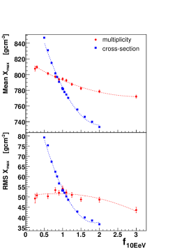
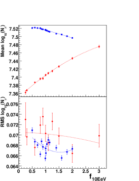
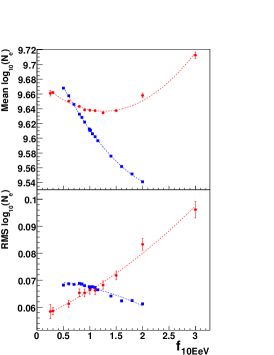
Figure 4: Mean and RMS values for the resulting $X_{\rm max}$, $\left.N_{\mu}(X)\right|_{X=1000\textrm{~{}gcm}^{-2}}$ and $\left.N_{\rm e}(X)\right|_{X=1000\textrm{~{}gcm}^{-2}}$ distributions as a function of $f_{\rm 10EeV}$ using SIBYLL 2.1. For each data point with changed multiplicity, 1000 air showers are simulated and 10000 for a changed cross section. The dashed lines are polynomial fits of 2^nd order to guide the eye.

To explore the impact of uncertainties of the present high energy hadronic interaction models on the interpretation of EAS observables, we modified the CONEX [20] program to change some of the interaction characteristics during EAS simulation. To achieve this, individual hadronic interaction characteristics are altered by the energy-dependent factor

$$f(E)=\left\{\begin{array}[]{l l}1&\quad\mbox{{E}$\leq$1~{}PeV}\\ 1+(f_{\rm 10EeV}-1)\cdot\log_{10}(E/1\rm{PeV})/\log_{10}(10\rm{EeV}/1\rm{PeV})&\quad\mbox{{E}$>$1~{}PeV}\end{array}\right.$$ (9)

which was chosen to be $1$ below 1 PeV, because at these energies accelerator data is available (Tevatron corresponds to 1.8 PeV). Above 1 PeV, $f(E)$ increases logarithmically with energy, reaching the value of $f_{\rm 10EeV}$ at 10 EeV.
The factor $f(E)$ is then used to re-scale specific characteristic properties of the high energy hadronic interactions such as the interaction cross section, secondary particle multiplicity or inelasticity. Obviously by doing this we may leave the parameter space allowed by the original model, but nevertheless one can get a clear impression of how the resulting EAS properties are depending on the specific interaction characteristics.
We demonstrate the impact of a changing multiplicity $n_{\rm mult}$ and cross section $\sigma$ on the following, important air shower observables: shower maximum $X_{\rm max}$, and the total number of electrons $N_{\rm e}^{\rm rec}$, as well as muons $N_{\mu}^{\rm rec}$ arriving at an observation level of $X_{\rm obs}=1000$ gcm^-2. Figure 3 shows the range of extrapolations of $n_{\rm mult}$ used by the current hadronic interaction models and thus motivates the energy dependent re-scaling of $n_{\rm mult}$ by $0.3\geq f_{\rm 10EeV}\geq 3$.
All simulations are performed for primary protons at 10 EeV using the SIBYLL 2.1[17] interaction model. Figure 4 summarizes the results, which are discussed below.
Multiplicity of secondary particle production
The effect of a changed multiplicity on the $X_{\rm max}$-distribution is a shift to shallower $X_{\rm max}$ with increasing $n_{\rm mult}$. This is what is already predicted by the extended Heitler model [21]

$$X_{\rm max}\propto\lambda_{r}\cdot\ln\frac{E_{0}}{n_{\rm mult}\cdot E^{\;\rm e.m.}_{\rm crit}},$$ (10)

where $\lambda_{r}$ is the electromagnetic radiation length and $E^{\;\rm e.m.}_{\rm crit}$ the critical energy in air. This is a consequence of the distribution of the same energy onto a growing number of particles. The resulting lower energy electromagnetic sub-showers reach their maximum earlier. The impact on the RMS of the $X_{\rm max}$-distribution is small, but there is a trend to smaller fluctuations for an increasing number of secondaries.
The total muon number after 1000 gcm^-2 of shower development is rising if the multiplicity increases. This reflects the overall increased number of particles. The fluctuations are not significantly affected.
More interesting is the impact on the electron number $N_{\rm e}^{\rm rec}$, which shows a minimum close to $f_{\rm 10EeV}=1$. The rising trend in the direction of smaller $n_{\rm mult}$ can be explained by the increase of $X_{\rm max}$ and therefore the shower maximum coming closer to the observation level. On the other hand the rising trend in the direction of larger $n_{\rm mult}$ is again just the consequence of a generally growing number of particles. In contrary to the muon number the RMS does significantly change while $n_{\rm mult}$ gets larger. This can be explained by the strong dependence of fluctuations in $N_{\rm e}^{\rm rec}$ from the distance to the shower maximum.
Cross section
By construction, scaling the cross section does affect all hadronic interactions above 1 PeV, not only the first interaction.
The mean as well as the RMS of the $X_{\rm max}$-distribution are decreasing with an increasing cross section. The effect is very pronounced, since the depth of the first interaction $X_{\rm 1}$ is affected as well as the shower startup phase. Both effects are pointing to the same direction. This makes $X_{\rm max}$ a very sensitive observable for a cross section measurement.
The impact on the muon number $N_{\mu}^{\rm rec}$ is not very large. Since the shower maximum moves away from the observation level with increasing cross section, we just see the slow decrease of the muon number at late shower development stages, while the fluctuation of $N_{\mu}^{\rm rec}$ stay basically constant.
The mean electron number as well as its fluctuations depend strongly on the distance of $X_{\rm max}$ from the observation level. Combined with the influence of the modified cross section on $X_{\rm max}$ this explains well the strong decrease of the mean $N_{\rm e}^{\rm rec}$ as well as the RMS with increasing cross section. At very small cross sections the shower maximum comes very close to the observation level, which can be observed as a flattening in the mean $N_{\rm e}^{\rm rec}$ and the decrease of the fluctuations in $N_{\rm e}^{\rm rec}$ against the trend of increasing fluctuations of the position of the shower maximum itself.

4 Summary

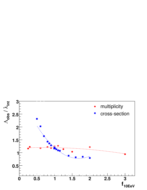
Figure 5: Simulated $k_{\rm X}$-factors ($k_{\rm X}=\Lambda^{\rm X}_{\rm obs}/\lambda_{\rm int}$) for SIBYLL at 10 EeV with modified cross section and multiplicity. $\Lambda_{\rm obs}^{\rm X}$ is obtained by an exponential fit to the tail of the resulting CONEX $X_{\rm max}$-distribution. An ideal detector is assumed, hence $k_{\rm X}=k_{\Delta X_{\rm 1}}$. The polynomial fits of 2^nd order are only plotted to guide the eye.

All methods of EAS-based cross section measurements are very similar and thus suffer from the same limitations.

• The values of all $k$-factors must be retrieved from massive Monte-Carlo simulations. All analysis attempts so far have only calculated the combined factor of $k_{\rm S}$, respectively $k_{\rm X}$.

• $k$-factors depend on the resolution of the experiment and can therefore not be transferred simply to other experiments.

• $k_{\rm X}$-factors are inherently different from $k_{\rm S}$-factors and can therefore not be transferred from an $X_{\rm max}$-tail analysis to that of ground based frequency attenuation or vice versa.

• It cannot be disentangled whether a measurement of $\Lambda_{\rm obs}$ can be attributed to $\lambda_{\rm int}$ entirely or at least partly to changed fluctuations in $\Delta X_{\rm 1}$ and/or $\Delta X_{\rm 2}$.

• Generally the $P_{\rm 1}$ and $P_{\rm 2}$ distributions have a complex shape and therefore the integrations of (3) and (6) to yield the approximations (5) and (8) are leading to non-exponential contributions.

• Any non-exponential contribution creates a strong dependence of the fitted $\Lambda_{\rm obs}$ on the chosen fitting range [22]. A strong non-exponential contribution makes the $k$-factor analysis unusable.

• It can be shown that the $P_{\rm 1}(\Delta X_{\rm 1})$-distributions is very sensitive to changes of the high energy hadronic interaction characteristics and thus $P(\Delta X)=f(\sigma,n_{\rm mult},...)$ is a function of $\sigma$ , $n_{\rm mult}$ and other high energy model parameters. Consequently this also makes the $k$-factors depending on the high energy interaction characteristics $k=f(\sigma,n_{\rm mult},...)$, which certainly must be considered for any cross section analysis.

In Fig. 5 we show how the here presented simulations can be used to quantify the uncertainty caused in the $k$-factors due to the dependence on $n_{\rm mult}$ to about $\pm\sim 0.1$ for a variation of the multiplicity by a factor from 0.3 up to 3. It is clear that even without considering the multiplicity as a possible source of uncertainty the $\sigma$-dependence of the $k$-factors certainly needs to be taken into account. Otherwise a systematic shift will be introduced into the resulting $\sigma_{\rm p-air}$, since part of the observed signal in $\Lambda_{\rm obs}$ is wrongly assigned to $\lambda_{\rm int}$, while in fact it must be attributed to $k(\sigma,n_{\rm mult},\dots)$ [23]. This has not been considered in any EAS-based $\sigma_{\rm p-air}$ measurement so far.

References

- [1] N. L. Grigorov et al. (1965). Proc. of 9th Int. Cosmic Ray Conf. (London), vol. 1, p. 860
- [2] G. B. Yodh, Y. Pal, and J. S. Trefil, Phys. Rev. Lett. 28, 1005 (1972)
- [3] R. A. Nam, S. I. Nikolsky, V. P. Pavluchenko, A. P. Chubenko, and V. I. Yakovlev (1975). In Proc. of 14th Int. Cosmic Ray Conf. (Munich), vol. 7, p. 2258
- [4] F. Siohan et al., J. Phys. G4, 1169 (1978)
- [5] H. H. Mielke, M. Föller, J. Engler, and J. Knapp, J. Phys. G 20, 637 (1994)
- [6] R. M. Baltrusaitis et al., Phys. Rev. Lett. 52, 1380 (1984)
- [7] M. Honda et al., Phys. Rev. Lett. 70, 525 (1993)
- [8] M. Aglietta et al. (1999). In Proc. of 26th International Cosmic Ray Conference (ICRC 99), Salt Lake City, Utah, 17-25 Aug 1999, vol. 1, p. 143
- [9] T. Hara et al., Phys. Rev. Lett. 50, 2058 (1983)
- [10] S. P. Knurenko, V. R. Sleptsova, I. E. Sleptsov, N. N. Kalmykov, and S. S. Ostapchenko (1999). In Proc. of 26th International Cosmic Ray Conference (ICRC 99), Salt Lake City, Utah, 17-25 Aug 1999, vol. 1, p. 372-375
- [11] K. Belov, Nucl. Phys. Proc. Suppl. 151, 197 (2006)
- [12] J. Ranft, Phys. Rev. D51, 64 (1995)
- [13] T. Pierog and K. Werner (2006). astro-ph/0611311
- [14] H. J. Drescher, M. Hladik, S. Ostapchenko, T. Pierog, and K. Werner, Phys. Rept. 350, 93 (2001). hep-ph/0007198
- [15] N. N. Kalmykov, S. S. Ostapchenko, and A. I. Pavlov, Nucl. Phys. Proc. Suppl. 52B, 17 (1997)
- [16] S. Ostapchenko, Phys. Rev. D74, 014026 (2006). hep-ph/0505259
- [17] R. Engel, T. K. Gaisser, T. Stanev, and P. Lipari (1999). In Proc. of 26th International Cosmic Ray Conference (ICRC 99), Salt Lake City, Utah, 17-25 Aug 1999, p. 415-418
- [18] R. S. Fletcher, T. K. Gaisser, P. Lipari, and T. Stanev, Phys. Rev. D50, 5710 (1994)
- [19] R. Ulrich, J. Blumer, R. Engel, F. Schussler, and M. Unger (2006). In Proc. of XIV ISVHECRI 2006, Weihai, China, 2006, astro-ph/0612205
- [20] T. Bergmann et al., Astropart. Phys. 26, 420 (2007). astro-ph/0606564
- [21] J. Matthews, Astropart. Phys. 22, 387 (2005)
- [22] J. Alvarez-Muniz, R. Engel, T. K. Gaisser, J. A. Ortiz, and T. Stanev, Phys. Rev. D69, 103003 (2004). astro-ph/0402092
- [23] R. Ulrich, J. Blumer, R. Engel, F. Schussler, and M. Unger (2007). In Proc. of 30th International Cosmic Ray Conference (ICRC 07), Merida, Mexico, 2007, 2007, vol. 1, p. 143, arXiv:0706.2086 [astro-ph].