Entanglement of Uniformly Accelerating Schrödinger, Dirac, and Scalar Particles

Abstract

We study how the entanglement of an entangled pair of particles is affected when one or both of the pair is uniformly accelerated, while the detector remains in an inertial frame. We find that the entanglement is unchanged if all degrees of freedom are considered. However, particle pairs are produced when a relativistic particle is accelerated, and more bipartite systems emerge, the entanglements of some of which may change as the acceleration. In particular, the entanglement of a pair of accelerating fermions is transferred preferentially to the produced antiparticles when the acceleration is large, and the entanglement transfer is complete when the acceleration approaches infinity. However, no such entanglement transfer to the antiparticles is observed for scalar particles.

I Introduction

Entanglement is an important property of quantum mechanical systems. It is useful in the field of quantum information and quantum computing, such as in quantum teleportation qutele . It also finds many applications in quantum control qc and quantum simulations qs . Studying quantum entanglement in relativistic systems may give us insights on the relationship between quantum mechanics and general relativity. It has been shown that entanglement is Lorentz invariant adami ; alsing . However, an accelerating observer measures less entanglement than an inertial observer in both the scalar tele ; nb and fermion nf cases. This degradation in entanglement is due to the splitting of space-time, as a result of which the vacuum observed in one frame can become excited in another frame - the case of Unruh effect unruh . Classically, the trajectory of a uniformly accelerating particle observed by an inertial observer is the same as that of an inertial particle measured by a uniformly accelerating observer with appropriate acceleration. We are interested in how the acceleration of particles affects the entanglement of the originally entangled states.

In this paper, we analyze the entanglement of accelerating particles in three cases: a non-relativistic wave packet, scalar and fermion particles. We compare the entanglement of accelerating particles, as seen by an inertial detector, with that of inertial particles observed by an accelerating detector tele ; nb ; nf ; zhang . We find that when all degrees of freedom are considered, the entanglement is unchanged. However, pair production occurs when a relativistic particle accelerates, and there are new bipartite systems. We find that the entanglements of some of the new bipartite systems can depend on the acceleration. In particular, a pair of accelerating fermions transfer their entanglement preferentially to the produced antiparticles when the acceleration is large, and the entanglement transfer is complete when the acceleration approaches infinity. However, no such entanglement transfer to the antiparticles is observed for scalar particles.

This paper is organized as follows. In Sec. II, we add a potential term in the Schrödinger equation that would lead to uniform acceleration in the classical limit. Then we construct a wave packet solution and a two-body entangled wave function, and we calculate the entanglement by Schmidt decomposition sd as a function of acceleration. In Sec. III, we add the same potential term in the Klein-Gordon equation and Dirac equation. A wave packet solution can be obtained kgwp_0 to give an intuitive picture of how a relativistic particle accelerates and pair production occurs. We quantize the fields and use the in/out formalism to calculate the pair production, and we introduce the logarithmic negativity lne to calculate the entanglements in different bipartite systems. In Sec. IV, we consider the case when one or both Dirac particles are accelerated. Entanglements between different degrees of freedom are calculated and entanglement transfer to the antiparticles will be shown. In Sec. V, we calculate the particle spectrum for scalar particles, and the results are compared with those observed by an accelerating observer. We also repeat the calculation of entanglements in Sec. IV but for scalar particles. A summary and discussion of results and further work is given in Sec. VI.

II Accelerating schrödinger particles

A free non-relativistic particle with mass $m$ represented by a gaussian wave packet

$$\psi_{0}(x,t)=\frac{(8b/\pi)^{1/4}}{\sqrt{4b+2it/m}}\exp\left(-\frac{x^{2}}{4b+2it/m}\right)$$ (1)

satisfies the Schrödinger equation $(\hbar=c=1)$,

$$i\frac{\partial\psi}{\partial t}=\frac{-1}{2m}\frac{\partial^{2}\psi}{\partial x^{2}}.$$ (2)

It is reasonable to assume that the center of the wave packet follows the classical trajectory of the corresponding particle accwp . Therefore, when a linear potential is added to the Schrödinger equation,

$$i\frac{\partial\psi}{\partial t}=\frac{-1}{2m}\frac{\partial^{2}\psi}{\partial x^{2}}-max\psi,$$ (3)

we use an ansatz of the form

$$\psi(x,t)=\psi_{0}(x-x_{0}-v_{0}t-\frac{1}{2}at^{2},t)e^{iS(x,t)},$$ (4)

which when substituted into Eq. (3) produces an accelerating wave packet with

$$\frac{1}{m}S(x,t;v_{0},a)=v_{0}x+axt-\frac{1}{2}av_{0}t^{2}-\frac{1}{6}a^{2}t^{3}-\frac{1}{2}v_{0}^{2}t,$$ (5)

where $v_{0}$ and $a$ are treated as parameters that represent the initial velocity and acceleration in the classical limit.

We write down the two-body entangled wave functions as follows,

$$\Psi_{\pm}(x,y,t) = N[\psi(x,t;v_{1},a_{1})\psi(y,t;v_{2},a_{2})\pm\psi(x,t;v_{2},a_{1})\psi(y,t;v_{1},a_{2})],$$ (6)

where $N$ is the normalization factor. For simplicity, we have just set the masses, initial positions and widths of the two particles in the wave packet to be the same. If $a_{1}$ or $a_{2}$ $\neq$ 0, the two-body wave function accelerates in a specific direction (see Figs. 1 and 2 for examples).

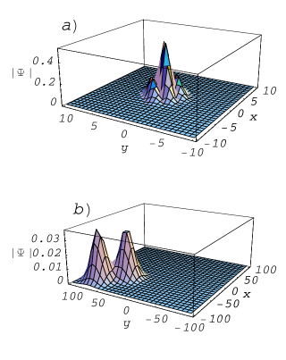
Figure 1: a) A 3D plot of the absolute value of the two-body wave function $\Psi_{+}$ Eq. (6) at $t$ = 0, for $v_{1}$ = -1, $v_{2}$ = 1, $x_{1}$ = $x_{2}$ = 0, $m_{1}$ = $m_{2}$ = 1, $a_{1}$ = -0.5, $a_{2}$ = 0.5. b) Same as Fig. 1a, but for $t$ = 15.

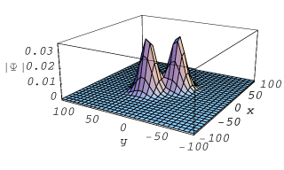
Figure 2: Same as Fig. 1b, but for $a_{1}$ = $a_{2}$ = 0 (free evolution).

We can calculate the purity $P$ of the wave function

$$P = \int\int\int\int\Psi(x,y,t)\Psi(x^{\prime},y^{\prime},t)\Psi^{*}(x,y^{\prime},t)\Psi^{*}(x^{\prime},y,t)dxdx^{\prime}dydy^{\prime},$$ (7)

and hence the Schmidt number: $K\equiv 1/P$. For a product state, $K=1$, and for entangled states, $K$ is greater than 1. The entanglement depends on the relative velocity of the two particles $v$ instead of the velocity of each of the particles. Therefore, we can choose to calculate the entanglement in the frame that $v_{1}$ = 0 and $v_{2}$ = $v$. The Schmidt number for $\Psi_{+}(x,y,t)$ is calculated to be (see Fig. 3)

$$K_{+}=\frac{2}{1+{4f}/{(1+f)^{2}}},$$ (8)

where $f=\exp(-\tilde{v}^{2})$ and $\tilde{v}\equiv vm\sqrt{b}$. In this case, the entanglement depends only on the product $bv^{2}m^{2}$ and is independent of the acceleration. This result can be easily understood. In the wave function, $a$ appears always as a product with $t$. As the Hamiltonian is Hermitian, the evolution operator is unitary, and the entanglement is unchanged under a unitary transformation. Thus we can choose to calculate the entanglement at time $t$ = 0, and all the acceleration terms will disappear. For $\Psi_{+}$, $K_{+}$ is equal to 1 when $v$ is equal to 0, and $K_{+}$ is equal to 2 when $v$ tends to infinity. For $\Psi_{-}$, $K_{-}$ is always equal to 2. Although the entanglement is independent of acceleration in both cases, there is a difference between the entanglements of $\Psi_{+}$ and $\Psi_{-}$. The entanglement depends on the orthogonality of the two terms in $\Psi_{\pm}$. For $\Psi_{+}$, a greater $v$ increases the orthogonality of the two terms in the wavefunction. The minus sign in $\Psi_{-}$ cancels the overlap region between the two terms in Eq. (6), and the remaining parts are orthogonal. As a result, the entanglement of $\Psi_{-}$ is always maximum in the system.

Figure 3: The Schmidt numbers $K_{\pm}$ as function of the relative velocity of the two particles, made dimensionless by  $\tilde{v}\equiv vm\sqrt{b}$, of the two-body wave functions $\Psi_{\pm}$.

III Relativistic Formalism

III.1 Quantization of Fields

In order to accelerate a relativistic particle, the Klein-Gordon (KG) or Dirac equation with an electric field is considered. A strong electric field makes the vacuum unstable and leads to pair production  fs ; wh ; jsch , which has been studied in the time dependent gauge pptg_1 ; pptg_2 , in Rindler coordinates  ppr and in a finite region  ppf_1 ; ppf_2 ; ppf_3 .

The pair production of scalar particles can be understood in the picture of a wave packet  kgwp_0 ; kgwp_1 . A wave packet uniformly accelerates from the far past, and then tunneling occurs in the region when it meets the potential barrier. The transmission wave packet represents the antiparticles while the reflected wave packet represents the particles. Therefore, pair production occurs in the tunneling region, and this solves the Klein paradox  klein . Although the wave packet formalism is more intuitive, it is not clear how to construct a two-body entangled probability density in the Klein-Gordon field. Thus, we quantize the field and calculate the Bogoliubov coefficients in the in/out formalism.

III.1.1 Scalar Particles

The Klein-Gordon equation  kgwp_0 ; kgwp_1 for a unit-charged particle with mass $m$ in a uniform electric field $E$ is

$$(D_{\mu}D^{\mu}+m^{2})\phi=0,$$ (9)

where $D_{\mu}=\partial_{\mu}+iA_{\mu}$ and the gauge is chosen to be $A_{0}$ = $-Ex$ and $A_{x}$ = 0. We assume $\phi_{\omega}(t,x)=C\exp{(i\omega t)}\chi_{\omega}(x)$, and the spatial part solutions are parabolic cylinder functions, $D_{-a-\frac{1}{2}}(x)$. Details of obtaining the solutions are shown in Appendix A. Then we classify the solutions in the in/out basis kgwp_0 ; greiner , such that we have two complete bases to quantize the field as

$$\phi=\sum_{\omega}(a_{\omega}^{in}\phi_{\omega,p}^{in}+b_{\omega}^{in\dagger}\phi_{\omega,a}^{in*}),$$ (10)

or

$$\phi=\sum_{\omega}(a_{\omega}^{out}\phi_{\omega,p}^{out}+b_{\omega}^{out\dagger}\phi_{\omega,a}^{out*}),$$ (11)

where the subscripts $p$ and $a$ label the particles and antiparticles respectively. The operators $a_{\omega}^{in}$($b_{\omega}^{in\dagger}$) and $a_{\omega}^{out}$($b_{\omega}^{out\dagger}$) are the annihilation (creation) operators in the in-basis and out-basis, and they are related by the Bogoliubov transformation,

$$a_{\omega}^{out}=\alpha^{*}a^{in}_{\omega}-\beta^{*}b_{\omega}^{in\dagger},$$ (12)

$$b_{\omega}^{out}=\alpha^{*}b_{\omega}^{in}-\beta^{*}a_{\omega}^{in\dagger},$$

where

$$\alpha=\frac{\sqrt{2\pi}e^{-i\pi/4}e^{-\pi\mu^{2}/2}}{\Gamma(1/2+i\mu^{2})},$$ (13)

$$\beta=e^{i\pi/2}e^{-\pi\mu^{2}},$$

with $\mu^{2}=m^{2}/2E$, and

$$|\alpha|^{2}-|\beta|^{2}=1.$$ (14)

We can express the in-vacuum state as the linear combination of out states kgwp_0 as,

$$|0\rangle_{in}=\prod_{\omega}\frac{1}{\alpha}\exp\left[\left(-\frac{\beta^{*}}{\alpha}\right)a^{out\dagger}_{\omega}b^{out\dagger}_{\omega}\right]|0\rangle_{out}.$$ (15)

We let $\alpha=e^{i\phi_{1}}\cosh{r}$ and $\beta=e^{i\phi_{2}}\sinh{r}$, where $0<r\lesssim 0.88$ is a parameter related to acceleration, and we neglect the phase factors which do not affect the following calculations of entanglement. Taking the single-mode approximation, we get the in-vacuum state in terms of the out states,

$$|0_{p}\rangle_{in}=\frac{1}{\cosh{r}}\sum_{n=0}^{\infty}\tanh^{n}{r}|n_{p}\rangle_{out}|n_{a}\rangle_{out}.$$ (16)

Similarly the one-particle state is

$$|1_{p}\rangle_{in}=\frac{1}{\cosh^{2}{r}}\sum^{\infty}_{n=0}\tanh^{n}{r}\sqrt{n+1}|(n+1)_{p}\rangle_{out}|n_{a}\rangle_{out}.$$ (17)

III.1.2 Fermions

For a unit-charged fermion with mass $m$ coupled to an uniform electric field,

$$[\gamma^{\mu}(p_{\mu}-A_{\mu})-m]\psi=0,$$ (18)

where $A_{\mu}$ is the vector potential and $\gamma_{\mu}$ is the gamma matrix. Eq. (18) can be reduced to two Klein-Gordon equations which are shown in Appendix B. The solutions are still the parabolic cylinder functions. The in/out basis solution of the second order ODE is still the in/out basis solution of the Dirac equation Eq. (18). Therefore, we obtain the Bogoliubov coefficients, which have been calculated in Ref. niki ,

$$a_{n}^{out}=\alpha_{f}a_{n}^{in}-\beta_{f}^{*}b_{n}^{in\dagger},$$ (19)

$$b_{n}^{out\dagger}=\beta_{f}a_{n}^{in}+\alpha_{f}^{*}b_{n}^{in\dagger},$$

where

$$\beta_{f}=e^{-\pi\mu^{2}},$$ (20)

$$\alpha_{f}^{*}=-i\sqrt{\frac{2\pi}{\mu^{2}}}\frac{e^{-\pi\mu^{2}/2}}{\Gamma(i\mu^{2})},$$

with $\alpha_{f}$ and $\beta_{f}$ having the relation,

$$|\alpha_{f}|^{2}+|\beta_{f}|^{2}=1.$$ (21)

We let $\alpha_{f}$ = $\cos{r_{f}}e^{i\phi}$ and $\beta_{f}$ = $\sin{r_{f}}$, $r_{f}$ being a parameter with values between 0 and ${\pi}/{2}$ and related to the acceleration. Also, we can relate the incoming states with the outgoing states as in the case of an accelerating detector nf ,

$$|0_{p}\rangle_{in}=\cos{r_{f}}e^{-i\phi}|0_{p}\rangle_{out}|0_{a}\rangle_{out}-\sin{r_{f}}|1_{p}\rangle_{out}|1_{a}\rangle_{out},$$ (22)

$$|1_{p}\rangle_{in}=|1_{p}\rangle_{out}|0_{a}\rangle_{out}.$$

III.2 Logarithmic Negativities

The entanglement can be quantified by the logarithmic negativity ne_1 ; ne_2 . For a density operator $\rho_{A,B}$ corresponding to a bipartite system $A$ and $B$, we define the trace norm $||\rho_{A,B}||$ $\equiv$ $tr|\rho_{A,B}|$ = $tr\sqrt{\rho_{A,B}^{\dagger}\rho_{A,B}}$ and the negativity

$$N_{e}\equiv\frac{||\rho^{T_{A}}||-1}{2},$$ (23)

where $\rho^{T_{A}}$ is the partial transpose of $\rho_{A,B}$ with respect to the party A. $N_{e}$ can be calculated from the absolute value of the sum of the negative eigenvalues of $\rho^{T_{A}}$. Then the logarithmic negativity of the bipartite system $A$ and $B$ is defined by,

$$LN(\rho_{A,B})\equiv\log_{2}||2N_{e}+1||.$$ (24)

For a product state, $LN(\rho_{A,B})$ = 0, and for entangled states, $LN(\rho_{A,B})>0$.

IV Accelerating fermions

Initially, we have the incoming entangled state,

$$\Psi_{i}=\frac{1}{\sqrt{2}}\left[|0_{s,p}\rangle_{in}|0_{\omega,p}\rangle_{in}+|1_{s,p}\rangle_{in}|1_{\omega,p}\rangle_{in}\right].$$ (25)

Then either one or both of the particles in $\omega$ and $s$ modes are accelerated by the electric field, and the in states in Eq. (25) are replaced by the out states as in Eq. (22). If only the $\omega$ mode is accelerated, we have

$$\Psi_{f} = \frac{1}{\sqrt{2}}\left\{|0_{s,p}\rangle_{out}\right.\otimes\left[\cos{r_{f}}e^{-i\phi}|0_{\omega,p}\rangle_{out}|0_{\omega,a}\rangle_{out}-\sin{r_{f}}|1_{\omega,p}\rangle_{out}|1_{\omega,a}\rangle_{out}\right]$$

$$\left.+|1_{s,p}\rangle_{out}\otimes(|1_{\omega,p}\rangle_{out}|0_{\omega,a}\rangle_{out})\right\}.$$

If both the $s$ and $\omega$ modes are accelerated with the same $r_{f}$, we have

$$\Psi_{f} = \frac{1}{\sqrt{2}}\left\{\left[\cos{r_{f}}e^{-i\phi_{1}}|0_{s,p}\rangle_{out}|0_{s,a}\rangle_{out}\right.-\sin{r_{f}}|1_{s,p}\rangle_{out}|1_{s,a}\rangle_{out}\right]$$

$$\otimes\left[\cos{r_{f}}e^{-i\phi_{1}}|0_{\omega,p}\rangle_{out}|0_{\omega,a}\rangle_{out}-\sin{r_{f}}|1_{\omega,p}\rangle_{out}|1_{\omega,a}\rangle_{out}\right]$$

$$\left.+\left[(|1_{s,p}\rangle_{out}|0_{s,a}\rangle_{out})\otimes(|1_{\omega,p}\rangle_{out}|0_{\omega,a}\rangle_{out})\right]\right\}.$$

The degradation of entanglement in the case of an accelerating detector is due to the fact that some degrees of freedom have been traced out. An accelerating detector ’sees’ the space-time being split into two causally disconnected regions, and it cannot access information in one of them. We have verified explicitly that the entanglement between the particles in $s$ mode and $\omega$ mode is unchanged if there is no tracing out of any space-time region. On the other hand, in the case of accelerating particles, the detector, which is in an inertial frame, can access all degrees of freedom and the orthogonality of the states is unchanged; therefore, the entanglement of accelerating particles is unchanged.

However, more degrees of freedom are produced and we can calculate the entanglements between different bipartite systems. In Ref. adami , it was shown that entanglement is Lorentz invariant. If one traces out the momentum, the entanglement decreases, and the entanglement is transferred from the momentum to the spin degrees of freedom. We will show that entanglement transfer also occurs in accelerating fermions, from the particles to the produced antiparticles.

If only the particle in the $\omega$ mode is accelerated, we can study the three bipartite systems: $A$ = the $s$ mode, $B$ = the particles in the $w$ mode, the antiparticles in $w$ mode, or the entire $w$ mode including both the particles and antiparticles. The density matrices are called $\rho_{s,p}$, $\rho_{s,a}$, and $\rho_{s,(p,a)}$ respectively. The entanglements are

$$\left\{\begin{array}[]{ll}LN(\rho_{s,(p,a)})=1,&\\ LN(\rho_{s,p})=\textrm{log}_{2}(1+\cos^{2}{r_{f}}),&\\ LN(\rho_{s,a})=\textrm{log}_{2}(1+\sin^{2}{r_{f}}),&\end{array}\right.$$ (31)

which are plotted in Fig. 4. It is obvious that the entanglement of $\rho_{s,p}$ is transferred to $\rho_{s,a}$.

When both the $s$ and $\omega$ modes are accelerated with the same $r_{f}$, we can calculate the entanglements between the five bipartite systems: particles in $s$ mode and particles in $\omega$ mode ($\rho_{p,p}$), antiparticles in $s$ and antiparticles in $\omega$ ($\rho_{a,a}$), antiparticles in $s$ and particles in $\omega$ ($\rho_{a,p}$), particles in $s$ and antiparticles in $\omega$ ($\rho_{p,a}$), and the entire $s$ and $\omega$ modes ($\rho_{(p,a),(p,a)}$). The logarithmic negativities are

$$\left\{\begin{array}[]{ll}LN(\rho_{(p,a),(p,a)})=1,\\ LN(\rho_{p,p})=\textrm{log}_{2}\left[1+\cos^{4}{r_{f}}\right],\\ LN(\rho_{a,a})=\textrm{log}_{2}\left[1+\sin^{4}{r_{f}}\right],\\ LN(\rho_{p,a})=\textrm{log}_{2}\left[1+\cos^{2}{r_{f}}\sin^{2}{r_{f}}\right].\end{array}\right.$$ (36)

By symmetry, $LN(\rho_{a,p})=LN(\rho_{p,a})$. The results are shown in Fig. 4. The entanglement is transferred from $\rho_{p,p}$ not only to $\rho_{p,a}$, but also to $\rho_{a,a}$. In fact, when the acceleration of the particles tends to infinity, the entanglement is completely transferred to between the antiparticles $\rho_{a,a}$. Note that in both cases, the negativities of the subsystems add up to the that of the total system, i.e., $N_{e}[\rho_{s,(p,a)}]=N_{e}[\rho_{s,p}]+N_{e}[\rho_{s,a}]$, $N_{e}[\rho_{(p,a),(p,a)}]=N_{e}[\rho_{p,p}]+N_{e}[\rho_{a,a}]+N_{e}[\rho_{p,a}]+N_{e}[\rho_{a,p}]$.

Figure 4: Logarithmic negativities of several bipartite systems when one or both fermions are accelerated, the magnitude of which is parameterized by $r_{f}$. In both cases, the entanglement between the entire $s$ mode and $\omega$ mode is unchanged (dot-dashed line). The solid lines show the results when both particles are accelerated together, for three bipartite systems: particles in $s$ mode and particles in $\omega$ mode ($\rho_{p,p}$), particles in $s$ mode and antiparticles in $\omega$ mode ($\rho_{p,a}$), and antiparticles in $s$ mode and antiparticles in $\omega$ mode ($\rho_{a,a}$). For comparison, the dashed lines show the results when only the particle in the $\omega$ mode is accelerated, in which case the two bipartite systems are particle in $s$ mode and particles in $\omega$ ($\rho_{s,p}$), and particle in $s$ mode and antiparticles in $\omega$ ($\rho_{s,a}$).

V Accelerating scalar particles

V.1 Spectrum

The relation between the in states and out states for scalar particles is just the same as the relation between the Minkowski states and Rindler states in  tele ; nb . However, their spectra are different. For both cases of accelerating particles with an inertial observer and inertial particles with an accelerating observer, the spectra are

$$S_{\omega}=\vskip 12.0pt plus 4.0pt minus 4.0pt_{in}\langle 0|a_{\omega}^{out\dagger}a_{\omega}^{out}|0\rangle_{in}=\sinh^{2}{r}.$$ (37)

The spectrum of accelerating particles with an inertial observer is $S_{\omega}=\exp(-\pi m/a)$, where $a=E/m$ corresponds to the acceleration of the particle in the classical limit. However, a uniformly accelerating detector measures a spectrum $S_{\omega}=1/[\exp({2\pi|\omega|}/{a})-1]$. In the classical limit, the detectors observe the same particle trajectories; however, a uniformly accelerating detector measures a different spectrum of particles as that by an inertial detector on uniformly accelerating particles.

V.2 Entanglement

For scalar particles, we have the same initially entangled state in Eq. (25). If only the particle in $\omega$ mode is put in a uniform electric field, the entangled state becomes

$$\Psi_{f} = \frac{1}{\sqrt{2}}\left\{|0_{p,s}\rangle_{out}\otimes\left[\frac{1}{\cosh{r}}\sum_{n=0}^{\infty}\tanh^{n}{r}|n_{p,\omega}\rangle_{out}|n_{a,\omega}\rangle_{out}\right]+\right.$$

$$\left.|1_{p,s}\rangle_{out}\otimes\left[\frac{1}{\cosh^{2}{r}}\sum^{\infty}_{n=0}\tanh^{n}{r}\sqrt{n+1}|(n+1)_{p,\omega}\rangle_{out}|n_{a,\omega}\rangle_{out}\right]\right\}.$$

If both particles in $\omega$ and $s$ modes are put in the electric field with same $r$, we have,

$$\Psi_{f} =\frac{1}{\sqrt{2}}\left\{\frac{1}{\cosh^{2}{r}}\left[\sum_{n=0}^{\infty}\tanh^{n}{r}|n_{p,s}\rangle_{out}|n_{a,s}\rangle_{out}\right]\otimes\left[\sum_{n=0}^{\infty}\tanh^{n}{r}|n_{p,\omega}\rangle_{out}|n_{a,\omega}\rangle_{out}\right]\right.$$

$$\left.+\frac{1}{\cosh^{4}{r}}\left[\sum^{\infty}_{n=0}\tanh^{n}{r}\sqrt{n+1}|(n+1)_{p,s}\rangle_{out}|n_{a,s}\rangle_{out}\right]\right.$$

$$\left.\otimes\left[\sum^{\infty}_{n=0}\tanh^{n}{r}\sqrt{n+1}|(n+1)_{p,\omega}\rangle_{out}|n_{a,\omega}\rangle_{out}\right]\right\}.$$

More degrees of freedom have arisen due to pair production. Again, the entanglement between the entire $s$ and $\omega$ modes remains unchanged, such that $LN(\rho_{s,\omega})=LN(\rho_{s,(p,a)})=LN(\rho_{(p,a),(p,a)})=1$ for all $r$. This is because the Bogoliubov transformation is linear, and the orthogonality property of the states is unchanged.

Figure 5: Same as Fig. 4, but for scalar particles. Again, the entanglement of the entire $s$ mode and $\omega$ mode, indicated by the dot-dashed line, remains unchanged. Note that $LN(\rho_{s,a})=LN(\rho_{p,a})=LN(\rho_{a,a})=0$ for all $r$.

We calculate the entanglements of $\rho_{s,p}$, $\rho_{s,a}$, $\rho_{p,p}$, $\rho_{a,a}$ and $\rho_{p,a}$. To calculate the density matrix, $\rho_{s,p}$ ($\rho_{s,a}$), we trace over the antiparticles (particles). We take the partial transpose, $\rho_{s,p}^{T}$, by interchanging the s mode’s qubits to get an infinite block-diagonal matrix. The ($n$, $n+1$) block matrix is,

$$\frac{\tanh^{2n}{r}}{2\cosh^{2}{r}}\left(\begin{array}[]{cc}\frac{n}{\sinh^{2}{r}}&\frac{\sqrt{n+1}}{\cosh{r}}\\ \frac{\sqrt{n+1}}{\cosh{r}}&\tanh^{2}{r}\\ \end{array}\right).$$ (42)

Then we calculate the negative eigenvalues from each block matrix and obtain the logarithmic negativity of $\rho_{s,p}$,

$$LN(\rho_{s,p}) = \textrm{log}_{2}\left[\frac{1}{2\cosh^{2}{r}}+\sum_{n=0}^{\infty}\frac{\tanh^{2n}{r}}{2\cosh^{2}{r}}\sqrt{\left(\frac{n}{\sinh^{2}{r}}+\tanh^{2}{r}\right)^{2}+\frac{4}{\cosh^{2}{r}}}\right].$$ (43)

We also calculate the $LN(\rho_{p,p})$ numerically. The results are shown in Fig. 5.

In contrast to fermions, there is no entanglement transfer to the antiparticles for scalar particles, and $LN(\rho_{s,a})=LN(\rho_{p,a})=LN(\rho_{a,a})=0$ for all $r$, even though the entanglement between the particles in the $s$ and $\omega$ modes decreases as $r$ increases.

V.3 Entanglements if the Number of Produced Pairs is Restricted

However, if we constrain the number of pairs produced, $LN(\rho_{s,a})$, $LN(\rho_{p,a})$ and $LN(\rho_{a,a})$ are all nonzero. If only $M$ pairs can be produced in a mode,

$$|0\rangle_{in}=\frac{N_{1}}{\cosh{r}}\sum_{n=0}^{M}\tanh^{n}{r}|n_{p}\rangle_{out}|n_{a}\rangle_{out},$$ (44)

$$|1_{p}\rangle_{in}=\frac{N_{2}}{\cosh^{2}{r}}\sum^{M-1}_{n=0}\tanh^{n}{r}\sqrt{n+1}|(n+1)_{p}\rangle_{out}|n_{a}\rangle_{out},$$

where $N_{1}$ and $N_{2}$ are normalization factors,

$$N_{1}=\left({1-\tanh^{2M+2}{r}}\right)^{-1/2},$$ (45)

$$N_{2}=\left[{{1-(M+1)\tanh^{2M}{r}+M\tanh^{2M+2}{r}}}\right]^{-1/2}.$$

We take the partial transpose of $\rho_{s,p}$ which has $M$ diagonal block matrices and the $n$th block is,

$$\frac{\tanh^{2n-4}{r}}{2\cosh^{2}{r}}\left(\begin{array}[]{cc}\frac{N_{2}^{2}}{\cosh^{2}{r}}(n-1)&\frac{N_{2}N_{1}\tanh^{2}{r}}{\cosh{r}}\sqrt{n}\\ \frac{N_{2}N_{1}\tanh^{2}{r}}{\cosh{r}}\sqrt{n}&N_{1}^{2}\tanh^{4}r\end{array}\right).$$ (48)

We then sum up the negative eigenvalues of the $n$th blocks to calculate the logarithmic negativity

$$LN(\rho_{s,p}) = \textrm{log}_{2}\left\{1-\sum_{n=1}^{M}\frac{\tanh^{2n-4}{r}}{2\cosh^{2}{r}}\left[\frac{(n-1)N_{2}^{2}}{\cosh^{2}{r}}+{N_{1}^{2}\tanh^{4}{r}}-\right.\right.$$

$$\left.\left.\sqrt{\left[\frac{(n-1)N_{2}^{2}}{\cosh^{2}{r}}+{N_{1}^{2}\tanh^{4}{r}}\right]^{2}+\frac{4N_{1}^{2}N_{2}^{2}\tanh^{4}{r}}{\cosh^{2}{r}}}\right]\right\}.$$

The partial transpose of $\rho_{s,a}$ also has a block diagonal structure and only the last block

$$\frac{\tanh^{2n-2}{r}}{2\cosh^{2}{r}}\left(\begin{array}[]{cc}N_{1}^{2}&\frac{N_{1}N_{2}\tanh{r}}{\cosh{r}}\sqrt{n}\\ \frac{N_{1}N_{2}\tanh{r}}{\cosh{r}}\sqrt{n}&0\\ \end{array}\right)$$ (52)

contributes to the negative eigenvalue. Then the logarithmic negativity of $\rho_{s,a}$ is

$$LN(\rho_{s,a}) = \textrm{log}_{2}\left\{1-\frac{N_{1}^{2}\tanh^{2M-2}{r}}{2\cosh^{2}{r}}\left[1-\sqrt{1+\frac{4N_{2}^{2}M\tanh^{2}{r}}{N_{1}^{2}\cosh^{2}{r}}}\right]\right\}.$$ (53)

We show the results $M$ = 1 and 2 in Fig. 6. In both cases, $LN(\rho_{s,(p,a)})$ is equal to 1.

Figure 6: Same as Fig. 5, but for $M$ = 1 (solid lines) and $M$ = 2 (dashed lines), and $\rho_{s,a}$ is shown as well.

When $M$ is finite, the entanglement of $\rho_{s,a}$ is not zero and increases with $r$ while that of $\rho_{s,p}$ decreases with $r$. However, the entanglements of both $\rho_{s,p}$ and $\rho_{s,a}$ are reduced if more particles are produced ($M$ increases). The dependence of $LN(\rho_{s,p})$ and $LN(\rho_{s,a})$ on $M$ at infinite acceleration are shown in Fig. 7. Although the entanglement of $\rho_{s,p}$ decreases more for greater $M$, the entanglement of $\rho_{s,a}$ also decreases with a similar trend and goes to zero when $M\rightarrow\infty$. Therefore, there is no transfer of entanglement to the antiparticles for scalar particles when the number of produced pairs is not restricted.

Figure 7: Logarithmic negativity of $\rho_{s,p}$ and $\rho_{s,a}$ at infinite acceleration (r = 0.88) as a function of the number of produced pairs $M$.

We next calculate the case when both particles in $\omega$ and $s$ modes are put in the uniform electric field such that they are both accelerated and have the same $r$. In the out basis, the state in Eq. (25) becomes,

$$\Psi_{f}=\frac{1}{\sqrt{2}}\left\{\frac{N_{1}^{2}}{\cosh^{2}{r}}\left[\sum_{n=0}^{M}\tanh^{n}{r}|n_{p,s}\rangle_{out}|n_{a,s}\rangle_{out}\right]\otimes\left[\sum_{n=0}^{M}\tanh^{n}{r}|n_{p,\omega}\rangle_{out}|n_{a,\omega}\rangle_{out}\right]+\right.$$ (54)

$$\left.\frac{N_{2}^{2}}{\cosh^{4}{r}}\left[\sum^{M}_{n=0}\tanh^{n}{r}\sqrt{n+1}|(n+1)_{p,s}\rangle_{out}|n_{a,s}\rangle_{out}\right]\otimes\left[\sum^{M}_{n=0}\tanh^{n}{r}\sqrt{n+1}|(n+1)_{p,\omega}\rangle_{out}|n_{a,\omega}\rangle_{out}\right]\right\}.$$

Now, we can consider even more bipartite systems between the two modes. We calculate the entanglements between the particles or antiparticles in the $s$ mode and the particles or antiparticles in the $\omega$ mode, i.e., of $\rho_{p,p}$, $\rho_{a,a}$, $\rho_{p,a}$ and $\rho_{a,p}$ for the cases $M=1$ and $2$. As expected from symmetry, $LN(\rho_{p,a})$ is equal to $LN(\rho_{a,p})$. The results are shown in Figs. 8 and 9 for $M=1$ and $2$ respectively. As in the case when only one of the particles is accelerated, the entanglement between the particles in $s$ and $\omega$ modes is degraded when $M$ increases. It seems that entanglement transfer also occurs for scalar particles for finite $M$. However, in this case we note that the negativities of the $\rho_{a,a}$, $\rho_{p,a}$, $\rho_{a,p}$, and $\rho_{p,p}$ do not sum to a constant, and we cannot identify a causal relation between the decrease in entanglement between the particles and the increase in entanglement between the antiparticles. A more rigorous definition of entanglement transfer is needed before we can discuss the issue for scalar particles further.

Figure 8: Logarithmic negativities of different bipartite systems when the particles in both $\omega$ and $s$ modes are accelerated, indicated by $\rho_{p,p}$ (between the particles and particles), $\rho_{p,a}$ (between particles in $s$ and antiparticles in $\omega$ modes), and $\rho_{a,a}$ (between antiparticles in $s$ and $\omega$ modes), for $M=1$. For comparison, the previous results (shown in Fig. 6) when only the particle in $\omega$ is accelerated are plotted as dashed lines.

Figure 9: Same as Fig. 8, but for $M=2$.

VI Conclusion

We have studied how the entanglement of a pair of particles is affected when one or both of the pair is uniformly accelerated, as measured by an inertial detector, and compared the results with that of inertial particles observed by a uniformly accelerating detector. While there is a degradation of entanglement in the latter case due to the splitting of the space-time, the entanglement in the former case is unchanged by the acceleration when all degrees of freedom are considered. Furthermore, the spectrum of the uniformly accelerating particles is different from that seen by uniformly accelerating detectors.

When one of the particles - the one in $\omega$ mode - is uniformly accelerated, the entanglement is transferred to the produced antiparticles for fermions, while there is no such entanglement transfer for scalar particles. For scalar particles, when the number of produced pairs is restricted, the entanglement of $\rho_{s,a}$ increases with $r$. However, at any $r$, $LN(\rho_{s,a})$ decreases as $M$ increases and goes to zero when $M\rightarrow\infty$.

When both particles in $s$ and $\omega$ modes are uniformly accelerated (with the same $r$ or $r_{f}$), we have even more bipartite systems. For fermions, $\rho_{a,a}$ takes up all the entanglement at large acceleration. For scalar particles with restricted number of produced pairs, the entanglements of $\rho_{p,a}$ and $\rho_{a,a}$ increase with $r$. However, if there is no restriction of the number of produced pairs, no entanglement transfer to the antiparticles is observed for scalar particles.

Our results raise the possibility that when an entangled pair falls into a black hole, their entanglement may be partially transferred to the produced particles, which should not be ignored in considering the black hole information paradox. Studying quantum entanglement in curved space-time may therefore give us insights on the relation between quantum mechanics and general relativity.

Appendix A The bogoliubov coefficients in the scalar case

We assume the form of solution of Eq. (9) as

$$\phi_{\omega}(t,x)=Ce^{i\omega t}\chi_{\omega}(x),$$ (55)

where $C$ is a normalization constant, and we obtain from Eq. (9)

$$\left[\frac{\partial^{2}}{\partial x^{2}}+E^{2}(x-\omega/E)^{2}\right]\chi_{\omega}(x)=m^{2}\chi_{\omega}(x).$$ (56)

The solutions of Eq. (56) can be found in  hand , and they are parabolic cylinder functions,

$$D_{i\mu^{2}-\frac{1}{2}}[\pm(1+i)\sqrt{E}(x-\omega)/E],$$ (57)

$$D_{-i\mu^{2}-\frac{1}{2}}[\pm(1-i)\sqrt{E}(x-\omega)/E].$$

We can use the saddle point method to classify the solutions in the in/out basis  kgwp_0 ; greiner and have the in-basis functions,

$$\phi^{in}_{\omega,p}(x,t)=\frac{e^{-3\pi\mu^{2}/4}}{(2E)^{1/4}}e^{i\omega t}D_{i\mu^{2}-1/2}[e^{-3i\pi/4}\sqrt{2E}(x-\omega/E)],$$ (58)

$$\phi^{in}_{\omega,a}(x,t)=\phi^{in}_{-\omega,p}(-x,t),$$ (59)

where $\mu^{2}=m^{2}/2E$. The subscripts $p$ and $a$ stand for particles and antiparticles respectively. We also obtain the out-basis solutions,

$$\phi^{out}_{\omega,p}(x,t)=\phi^{in*}_{\omega,p}(x,-t),$$ (60)

$$\phi^{out}_{\omega,a}(x,t)=\phi^{in*}_{-\omega,p}(-x,-t).$$ (61)

The solutions have been normalized by the Klein-Gordon scalar product,

$$\int dx\phi_{\omega^{{}^{\prime}},p}^{in*}(x,t)i\overleftrightarrow{D_{t}}\phi_{\omega,p}^{in}(x,t)=+\delta(\omega-\omega^{{}^{\prime}}),$$ (62)

$$\int dx\phi_{\omega^{{}^{\prime}},a}^{in*}(x,t)i\overleftrightarrow{D_{t}}\phi_{\omega,a}^{in}(x,t)=-\delta(\omega-\omega^{{}^{\prime}}).$$

As there are two different complete bases, we can quantize the field in two ways,

$$\phi=\sum_{\omega}(a_{\omega}^{in}\phi_{\omega,p}^{in}+b_{\omega}^{in\dagger}\phi_{\omega,a}^{in*}),$$ (63)

or

$$\phi=\sum_{\omega}(a_{\omega}^{out}\phi_{\omega,p}^{out}+b_{\omega}^{out\dagger}\phi_{\omega,a}^{out*}).$$ (64)

From hand , we can get a relation between the out-basis and in-basis solutions,

$$D_{-\frac{1}{2}-i\mu^{2}}[-(1+i)\sqrt{E}(x-\omega/E)]$$ (65)

$$=e^{-\pi\mu^{2}+\frac{i\pi}{2}}D_{-\frac{1}{2}-i\mu^{2}}[(1+i)\sqrt{E}(x-\omega/E)]+\frac{\sqrt{2\pi}e^{-i\pi/4}e^{-\pi\mu^{2}/2}}{\Gamma(\frac{1}{2}+i\mu^{2})}D_{-\frac{1}{2}+i\mu^{2}}[-(1-i)\sqrt{E}(x-\omega/E)].$$

We write Eq. (65) in the form of in-basis and out-basis solutions explicitly,

$$\phi_{\omega,p}^{out}=\beta\phi_{\omega,a}^{in*}+\alpha\phi_{\omega,p}^{in}.$$ (66)

Since $\beta=e^{i\phi_{2}}\sinh{r}$, $r=\sinh^{-1}[\exp(-\pi m/2a)]$.

Appendix B Reducing the Dirac equations to two Klein-Gordon equations

From Eq. (18), we let

$$\psi=(\gamma^{\nu}(p_{\mu}-A_{\mu})+m)\phi$$ (67)

to obtain

$$[(p-A)^{2}-m^{2}-{i}\sigma^{\mu\nu}(p_{\mu}-A_{\mu})(p_{\nu}-A_{\nu})]\phi=0,$$ (68)

where $\sigma^{\mu\nu}={i[\gamma^{\mu},\gamma^{\nu}]}/{2}$. We choose the gauge to be $A_{0}=0$, $A_{3}=-Et$. We then substitute the potential in Eq. (68) to get

$$\left[-\frac{\partial^{2}}{\partial t^{2}}-\left(i\frac{\partial}{\partial z}+Et\right)^{2}-m^{2}+iE\alpha_{3}\right]\phi=0,$$ (69)

where

$$\alpha_{3}=\left(\begin{array}[]{cc}0&\sigma_{3}\\ \sigma_{3}&0\\ \end{array}\right),$$ (72)

and $\sigma_{3}$ is the Pauli matrix. We then assume that the solution has the form

$$\phi=e^{ikz}n(t),$$ (73)

where

$$n(t)=\sum^{4}_{\lambda=1}f_{\lambda}(t)u_{\lambda},$$ (74)

with the spinors,

$$u_{1}=\frac{1}{\sqrt{2}}\left(\begin{array}[]{c}1\\ 0\\ 1\\ 0\\ \end{array}\right),u_{2}=\frac{1}{\sqrt{2}}\left(\begin{array}[]{c}0\\ 1\\ 0\\ -1\\ \end{array}\right),$$ (83)

$$u_{3}=\frac{1}{\sqrt{2}}\left(\begin{array}[]{c}1\\ 0\\ -1\\ 0\\ \end{array}\right),u_{4}=\frac{1}{\sqrt{2}}\left(\begin{array}[]{c}0\\ 1\\ 0\\ 1\\ \end{array}\right).$$ (92)

With the relations,

$$\alpha_{3}u_{\lambda}=\eta u_{\lambda},\left\{\begin{array}[]{ll}\eta=1,&\hbox{for }\lambda=1,2,\\ \eta=-1,&\hbox{for }\lambda=3,4,\end{array}\right.$$ (95)

we can get two Klein-Gordon equations,

$$\left[\frac{\partial^{2}}{\partial t^{2}}+E^{2}\left(t-\frac{k}{E}\right)^{2}+m^{2}-iE\eta\right]f_{\lambda}(t)=0.$$ (96)

The solutions are parabolic cylinder functions.

We can then classify the in/out solutions kgwp_1 ; Aniki . $f_{3}$ and $f_{4}$ are dependent on $f_{1}$ and $f_{2}$, and so we just consider the cases of $\lambda=1,2$ in the following. Neglecting the normaliazation factors, we write down the in/out solutions,

$$\begin{array}[]{ll}&\phi_{p}^{in}=e^{ikz}D_{i\mu^{2}}[-(1-i)\sqrt{E}(t-k/E)],\\ &\phi_{a}^{in}=e^{ikz}D_{-i\mu^{2}-1}[-(1+i)\sqrt{E}(t-k/E)],\\ &\phi_{p}^{out}=e^{ikz}D_{-i\mu^{2}-1}[(1+i)\sqrt{E}(t-k/E)],\\ &\phi_{a}^{out}=e^{ikz}D_{i\mu^{2}}[(1-i)\sqrt{E}(t-k/E)],\end{array}$$ (101)

where $\mu^{2}=m^{2}/2E$. We substitute the solutions in Eq. (101) into Eq. (67), to obtain the solutions in the Dirac equation, i.e., Eq. (18). We show the calculation of $\phi_{p}^{in}$ with $\lambda=1$ as follows.

$$\psi_{p,1}^{in} = \left[\gamma^{\mu}(p_{\mu}-A_{\mu})+m\right]u_{1}e^{ikz}D_{i\mu^{2}}[-(1-i)\sqrt{E}(t-k/E)]$$

$$= e^{ikz}\left[mu_{1}D_{i\mu^{2}}[-(1-i)\sqrt{E}(t-{k}/{E})]-(1-i)\mu^{2}\sqrt{E}u_{1}^{{}^{\prime}}D_{i\mu^{2}-1}[-(1-i)\sqrt{E}(t-{k}/{E})]\right],$$

where $u_{1}^{{}^{\prime}}=\gamma^{0}u_{1}=\gamma^{3}u_{1}$. We normalize it and calculate $\psi_{a}^{in}$, $\psi_{p}^{out}$ and $\psi_{a}^{out}$. We can relate the solutions using two mathematical relations

$$D_{i\mu^{2}-1}[(1-i)x]=-e^{-{\pi\mu^{2}}}D_{i\mu^{2}-1}[-(1-i)x]+\frac{\sqrt{2\pi}e^{-\pi\mu^{2}/2}}{\Gamma(1-{i\mu}^{2})}D_{-i\mu^{2}}[-(1+i)x],$$ (103)

$$D_{i\mu^{2}}[(1-i)x]=e^{-{\pi\mu^{2}}}D_{i\mu^{2}}[-(1-i)x]+\frac{i\sqrt{2\pi}e^{-\pi\mu^{2}/2}}{\Gamma(-{i\mu}^{2}/{2})}D_{-1-i\mu^{2}}[-(1+i)x],$$

and so we can obtain the Bogoliubov coefficients,

$$\beta_{f}=e^{-\pi\mu^{2}},$$ (104)

$$\alpha_{f}^{*}=-i\sqrt{\frac{2\pi}{\mu^{2}}}\frac{e^{-\pi\mu^{2}/2}}{\Gamma(i\mu^{2})}.$$

Since $\beta_{f}=\sin{r_{f}}$, $r_{f}=\arcsin{[\exp(-\pi m/2a)]}$.

References

• (1) C. H. Bennett et al., Phys. Rev. Lett. 70, 1895 (1993).
• (2) S. F. Huelga, M. B. Plenio, and J. A. Vaccaro, Phys. Rev. A 65, 042316 (2002).
• (3) J. L. Dodd, M. A. Nielsen, M. J. Bremner, and R. T. Thew, Phys. Rev. A 65, 040301(R) (2002).
• (4) R. M. Gingrich and C. Adami, Phys. Rev. Lett. 89, 270402 (2002).
• (5) P. M. Alsing and G. J. Milburn, Quantum Inf. Comput. 2, 487 (2002); eprint quant-ph/0203051.
• (6) P. M. Alsing and G. J. Milburn, Phys. Rev. Lett. 91, 180404 (2003).
• (7) I. Fuentes-Schuller and R. B. Mann, Phys. Rev. Lett. 95, 120404 (2005).
• (8) P. M. Alsing, I. Fuentes-Schuller, R. B. Mann, and T. E. Tessier, quant-ph/0603269v2.
• (9) W. G. Unruh, Phys. Rev. D 14, 870 (1976).
• (10) Y. Ling et al., J. Phys. A: Math. Theor. 40, 9025 (2007).
• (11) S. Parker et al., Phys. Rev. A 61, 032305 (2000).
• (12) R. Brout, S. Massar, R. Parentani, and Ph. Spindel, Phys. Rep. 260, 329 (1995).
• (13) G. Vidal and R. F. Werner, Phys. Rev. A 65, 032314 (2002).
• (14) G. Vandegrift, Am. J. Phys. 68, 576 (2000).
• (15) F. Sauter, Z. Phys. 69, 742 (1931).
• (16) W. Heisenberg and H. Euler, Z. Phys. 98, 714 (1936).
• (17) J. Schwinger, Phys. Rev. 82, 664 (1951).
• (18) T. Padmanabhan, Pramana-Journal of Physics 37, 179 (1991).
• (19) K. Srinivasan and T. Padmanabhan, Phys. Rev. D 60, 024007 (1999).
• (20) Cl. Gabriel and Ph. Spindel, Ann. Phys. (N.Y.) 284, 263 (2000).
• (21) R.-C. Wang and C.-Y. Wong, Phys. Rev. D 38, 348 (1988).
• (22) C. Martin and D. Vautherin, Phys. Rev. D 38, 3593 (1988).
• (23) C. Martin and D. Vautherin, Phys. Rev. D 40, 1667 (1989).
• (24) R. Brout, S. Massar, R. Parentani, S. Popescu, and Ph. Spindel, Phys. Rev. D 52, 1119 (1995).
• (25) O. Klein, Z. Phys. 53, 157 (1929).
• (26) W. Greiner, B. Müller, and J. Rafelski, Quantum Electrodynamics of Strong Fields (Springer, Berlin, 1985).
• (27) A. Nikishov, Journal of Experimental and Theoretical Physics 96, 180 (2003).
• (28) M. B. Plenio, Phys. Rev. Lett. 95, 090503 (2005).
• (29) M. B. Plenio and S. Virmani, quant-ph/0504163v3.
• (30) M. Abramowitz and I. A. Stegun, Handbook of Mathematical Functions (Dover, New York, 1964).
• (31) A. I. Nikishov, Journal of Russian Laser Research 6, 1573 (1985).