PAIRING CORRELATIONS IN HALO NUCLEI

Abstract

Paring correlations in weakly bound halo nuclei ⁶He and ¹¹Li are studied by using a three-body model with a density-dependent contact interaction. We investigate the spatial structure of two-neutron wave function in a Borromean nucleus ¹¹Li. The behavior of the neutron pair at different densities is simulated by calculating the two-neutron wave function at several distances between the core nucleus ⁹Li and the center of mass of the two neutrons. With this representation, a strong concentration of the neutron pair on the nuclear surface is quantitatively established for neutron-rich nuclei. Dipole excitations in ⁶He and ¹¹Li are also studied within the same three-body model and compared with experimental data. The small open angles between the two neutrons from the core are extracted empirically by the B(E1) sum rule together with the rms mass radii, indicating the strong di-neutron correlation in the halo nuclei.

1 Introduction

Pairing correlations play a crucial role in many Fermion systems, such as liquid ³He, atomic nuclei, and ultracold atomic gases. When an attractive interaction between two Fermions is weak, the pairing correlations can be understood in terms of the well-known BCS mechanism, that shows a strong correlation in the momentum space. If the interaction is sufficiently strong, on the other hand, one expects that two Fermions form a Bosonic bound state and condense in the ground state of many-body system [1]. The transition from the BCS-type pairing correlation to the Bose-Einstein condensation (BEC) takes place continuously as a function of the strength of attractive interaction. This feature is referred to as the BCS-BEC crossover.

It has been feasible by now to study the structure of nuclei on the edge of neutron drip line. Such nuclei are characterized by a dilute neutron density around the nuclear surface so that one can investigate the pairing correlations at several densities[2], ranging from the normal density in the center of nucleus to a diluted density at the surface. The pairing correlations are predicted to be strong at the surface, but rather weak at the normal density and also far outside of the core. Thus, the weakly bound nuclei will provide an ideal environment to study the dynamics of pairing correlations in relation with the BCS-BEC crossover phenomenon.

In this talk, we discuss the manifestation of the BCS-BEC crossover phenomenon in finite neutron-rich nuclei. We particularly study the ground state wave function of a two-neutron halo nuclei, ⁶He and ¹¹Li. These nuclei are known to be well described as a three-body system consisting of two valence neutrons and the core nucleus(⁴He or ⁹Li) [3, 4, 5]. A strong di-neutron correlation as a consequence of pairing interaction between the valence neutrons has been shown theoretically in ¹¹Li [6, 5]. We take this nucleus to study BCS-BEC crossover features in connection to the strong two-neutron correlation, which has recently been observed experimentally in low-lying dipole strength in ¹¹Li [7].

2 Three-body model and di-neutron correlation

In order to study the pair wave function in ¹¹Li, we solve the following three-body Hamiltonian [6, 5],

$$H=\hat{h}_{nC}(1)+\hat{h}_{nC}(2)+V_{nn}+\frac{\vec{p}_{1}\cdot\vec{p}_{2}}{A_{c}m},$$ (1)

where $m$ and $A_{c}$ are the nucleon mass and the mass number of the inert core nucleus, respectively. $\hat{h}_{nC}$ is the single-particle Hamiltonian for a valence neutron interacting with the core. We use a Woods-Saxon potential for the interaction in $\hat{h}_{nC}$. The diagonal component of the recoil kinetic energy of the core nucleus is included in $\hat{h}_{nC}$, whereas the off-diagonal part is taken into account in the last term in the Hamiltonian (1). The interaction between the valence neutrons $V_{nn}$ is taken as a delta interaction whose strength depends on the density of the core nucleus. Assuming that the core density is described by a Fermi function, it reads

$$V_{nn}(\vec{r}_{1},\vec{r}_{2})=\delta(\vec{r}_{1}-\vec{r}_{2})\left(v_{0}+\frac{v_{\rho}}{1+\exp[(R-R_{\rho})/a_{\rho}]}\right),$$ (2)

where $R=|(\vec{r}_{1}+\vec{r}_{2})/2|$. We use the same value for the parameters as in Refs. [6, 5].

The two-particle wave function $\Psi(\vec{r}_{1},\vec{r}_{2})$ is obtained by diagonalizing the three-body Hamiltonian (1) with a large model space which is consistent with the $nn$ interaction, $V_{nn}$. To this end, we expand the wave function $\Psi(\vec{r}_{1},\vec{r}_{2})$ with the eigenfunction $\phi_{nljj_{z}}(\vec{r}_{i})$ of the single-particle Hamiltonian $\hat{h}_{nC}$. In the expansion, we explicitly exclude those states which are occupied by the core nucleus.

The ground state wave function is obtained as the state with the total angular momentum $J=J_{z}=0$. We transform it to the coordinate system with the relative and center of mass (cm) motions for the valence neutrons, $\vec{r}=\vec{r}_{1}-\vec{r}_{2}$ and $\vec{R}=(\vec{r}_{1}+\vec{r}_{2})/2$ [8, 9]. The wave function is first decomposed into the total spin $S$=0 and $S$=1 components. Then, the coordinate transformation is performed for the $S$=0 component, which is relevant to the pairing correlation:

$$\Psi^{S=0}(\vec{r}_{1},\vec{r}_{2})=\sum_{L}f_{L}(r,R)\,[Y_{L}(\hat{\vec{r}})Y_{L}(\hat{\vec{R}})]^{(00)}\,|\chi_{S=0}\rangle,$$ (3)

where $|\chi_{S=0}\rangle$ is the spin wave function. The two-particle wave function is plotted for ¹¹Li in two different coordinates in Fig. 1. Fig. 1(a) is plotted as a function of $r\equiv r_{1}=r_{2}$ and the angle between the valence neutrons, while the radial coordinates $r$ and $R$ are adopted for Fig. 1(c). The $S=0$ component is only taken for Fig. 1(b). One observes two peaks in both the figures. The peak at smaller angle $\theta_{12}$ in Fig. 1(a) is referred to as “di-neutron configuration” , while the large angle is called “cigar-like configuration”. One can see the di-neutron configuration has a long tail as a typical feature of halo wave function.

(a)

(b)

(c)

Figure 1: A two dimensional plot of the square of the ground state two-particle wave function for ¹¹Li; (a) the total density, (b) the $S=0$ component as a function of the radial coordinate $r\equiv r_{1}=r_{2}$ and the angle between the valence neutrons $\theta_{12}$. (c) $r^{2}R^{2}|f_{L=0}(r,R)|^{2}$ in Eq. (3), as a function of the relative distance $r$ and the center of mass coordinate $R$ for the valence neutrons as denoted in the upper right inset.

Figure 1 (c) shows the square of two-particle wave function for the $L=0$ component. One can clearly recognize the two peaked structure in the plot, corresponding to the di-neutron and the cigar-like configurations.

The $L=0$ wave functions of ¹¹Li for different values of $R$ are plotted in Fig. 2. Since we consider the density-dependent contact interaction, Eq. (2), this is effectively equivalent to probing the wave function at different densities. At $R=0.5$ fm, where the density is close to the normal density $\rho_{0}$, the two particle wave function is spatially extended and oscillates inside the nuclear interior. This oscillatory behavior is typical for a Cooper pair wave function in the BCS approximation, and has in fact been found in nuclear and neutron matters at normal density $\rho_{0}$ [10, 11]. As $R$ increases, the density $\rho$ decreases. The two-particle wave function then gradually deviates from the BCS-like behavior. At $R=3$ fm, the oscillatory behavior almost disappears and the wave function is largely concentrated inside the first node at $r\sim$ 4.5 fm. The wave function is compact in shape, indicating the strong di-neutron correlation, typical for BEC where many such pairs are present. At $R$ larger than 3 fm, the squared wave function has essentially only one node, and the width of the peak gradually increases as a function of $R$. This behavior is qualitatively similar to the pair wave function in infinite matter [10]. We have confirmed using the same three-body model that this scenario also holds for another Borromean nucleus ⁶He as well as for non-Borromean neutron-rich nuclei ¹⁶C and ²⁴O.

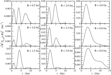
Figure 2: The ground state two-particle wave functions, $r^{2}R^{2}|f_{L=0}(r,R)|^{2}$ of ¹¹Li as a function of the relative distance between the neutrons, $r$, at several center of mass distances $R$ as indicated in the inset. Notice the different scales on the ordinate in the various panels.

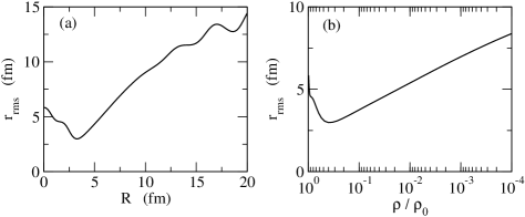
Figure 3: The root mean square distance $r_{\rm rms}$ for the neutron pair.

The transition from the BCS-type pairing to the BEC-type di-neutron correlation can also clearly be seen in the root mean square (rms) distance of the two neutron system. We plot this quantity in Fig. 3(a) as a function of $R$. In order to compare it with the rms distance in nuclear matter, we relate the cm distance $R$ with the density $\rho$ using the Fermi-type functional form $\rho(R)/\rho_{0}=[1+\exp((R-R_{\rho})/a_{\rho})]^{-1}$, as used in the $nn$ interaction in Eq. (2). Fig. 3(b) shows the rms distance as a function of density $\rho$ thus obtained. The rms distance shows a distinct minimum at $\rho\sim 0.4\rho_{0}$ ($R\sim$ 3.2 fm). This indicates that the strong di-neutron correlation grows in ¹¹Li around this density. Notice that the probability to find the two-neutron pair is maximal around this region (see Fig. 1 (c)). The behavior of rms distance as a function of density $\rho$ qualitatively well agrees with that in infinite matter (see Fig. 3 in Ref. [10]), although the absolute value of the rms distance is much smaller in the finite nucleus.

3 Dipole excitations and correlation angles

The rms distance $\sqrt{\langle r^{2}_{c-2n}\rangle}$ has an intimate relation to the B(E1) strength as [3, 4, 12],

$$B(E1)=\frac{3}{\pi}\left(\frac{Ze}{A}\right)^{2}\,\langle r^{2}_{c-2n}\rangle.$$ (4)

This relation is obtained with closure, which includes unphysical Pauli forbidden transitions to the states with negative excitation energies. Although the effect of Pauli forbidden transitions is not large, it leads to a non-negligible correction. In Ref. [12, 13], it has been proposed to estimate the experimental value for $\langle r^{2}_{c-2n}\rangle$ using the relation,

$$\langle r^{2}_{c-2n}\rangle_{\rm exp}=\frac{B(E1;E\leq E_{\rm max})_{\rm exp}}{B(E1;E\leq E_{\rm max})_{\rm cal}}\,\cdot\langle r^{2}_{c-2n}\rangle_{\rm cal}.$$ (5)

The dipole strength distributions for the ⁶He and ¹¹Li nuclei obtained with the three model are shown in Fig. 4. Also shown by the solid curves are the B(E1) distributions smeared with the Lorenzian function with the width of $\Gamma=0.2$ MeV. For the ⁶He nucleus, we obtain the total B(E1) strength of 0.660 e²fm² up to $E\leq 5$ MeV and 1.053 e²fm² up to $E\leq 10$ MeV. These are in good agreement with the experimental values, B(E1; $E\leq$ 5 MeV)=0.59 $\pm$ 0.12 e²fm² and B(E1; $E\leq$ 10 MeV)=1.2 $\pm$ 0.2 e²fm² [15]. For the ¹¹Li nucleus, we obtain the total B(E1) strength of 1.405 e²fm² up to $E_{\rm rel}=E-S_{2n}\leq 3$ MeV, which is compared to the experimental value, B(E1; $E_{\rm rel}\leq$ 3 MeV)=1.42 $\pm$ 0.18 e²fm² [7]. Again, the experimental data is well reproduced within the present model. From the calculated values for $\langle r^{2}_{c-2n}\rangle_{\rm cal}$, that is, 13.2 and 26.3 fm² for ⁶He and ¹¹Li, respectively, we thus obtain $\sqrt{\langle r^{2}_{c-2n}\rangle_{\rm exp}}=3.878\pm 0.324$ fm and 5.15 $\pm$ 0.327 fm for ⁶He and ¹¹Li, respectively. Notice that the value for the ⁶He nucleus is somewhat larger than the one estimated in Ref. [15], that is, 3.36 $\pm$ 0.39 fm.

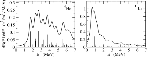
Figure 4: The B(E1) distribution for the ⁶He and ¹¹Li nuclei. The solid curve is obtained by a smearing procedure with a Lorentzian weighting factor of the width $\Gamma$=0.2 MeV.

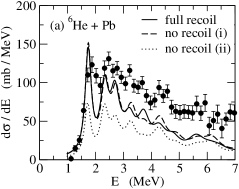
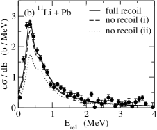
Figure 5: Coulomb breakup cross sections (a) for ⁶He+Pb at 240 MeV /nucleon, and (b) for ¹¹Li+Pb at 70 MeV /nucleon. The solid line is the result of the full three-body calculations, while the dashed and the dotted lines are obtained by treating the recoil term approximately (see Ref. [13] for details). These results are smeared with an energy dependent width of $\Gamma=0.15\cdot\sqrt{E_{\rm rel}}$ MeV. The experimental data are taken from Ref. [15] for ⁶He and from Ref. [7] for ¹¹Li.

We next evaluate the Coulomb breakup cross sections based on the relativistic Coulomb excitation theory [14]. These are obtained by multiplying the virtual photon number $N_{\rm E1}(E)$ to the B(E1) distribution shown in Fig. 4. The solid line in Figs. 5 (a) and (b) shows the Coulomb breakup cross sections thus obtained for ⁶He+Pb reaction at 240 MeV/nucleon [15] and ¹¹Li+Pb reaction at 70 MeV/nucleon [7], respectively. In order to facilitate the comparison with the experimental data, we smear the discretized cross sections with the Lorenzian function with an energy dependent width, $\Gamma=\alpha\cdot\sqrt{E_{\rm rel}}$. We take $\alpha=0.15$MeV^1/2 and 0.25 MeV^1/2 for ⁶He and ¹¹Li, respectively. We see that the experimental breakup cross sections are reproduced remarkably well within the present three-body model, especially for the ¹¹Li nucleus.

Let us now discuss the geometry of the ⁶He and ¹¹Li nuclei. Using the experimental value for $\langle r^{2}_{c-2n}\rangle$ obtained from the B(E1) distribution, one can extract the mean opening angle between the valence neutrons once an additional information is available. The mean opening angle can be extracted directly when the rms distance between the valence neutrons, $\langle r^{2}_{nn}\rangle$, is available. This quantity is related to the matter radius and $\langle r_{c-2n}^{2}\rangle$ in the three-body model [3, 6, 12],

$$\langle r_{m}^{2}\rangle=\frac{A_{c}}{A}\,\langle r_{m}^{2}\rangle_{A_{c}}+\frac{2A_{c}}{A^{2}}\,\langle r_{c-2n}^{2}\rangle+\frac{1}{2A}\,\langle r_{nn}^{2}\rangle,$$ (6)

where $A_{c}=A-2$ is the mass number of the core nucleus. The matter radii $\langle r_{m}^{2}\rangle$ can be estimated from interaction cross sections. Employing the Glauber theory in the optical limit, Tanihata et al. have obtained $\sqrt{\langle r_{m}^{2}\rangle}$ = 1.57 $\pm$ 0.04, 2.48 $\pm$ 0.03, 2.32 $\pm$ 0.02, and 3.12 $\pm$ 0.16 fm for ⁴He, ⁶He, ⁹Li, and ¹¹Li, respectively [16]. Using these values, we obtain the rms neutron-neutron distance of $\sqrt{\langle r_{nn}^{2}\rangle}$ = 3.75 $\pm$ 0.93 and 5.50 $\pm$ 2.24 fm for ⁶He and ¹¹Li, respectively. Combining these values with the rms core-di-neutron distance, $\sqrt{\langle r_{c-2n}^{2}\rangle}$, obtained with Eq. (5), we obtain the mean opening angle of $\langle\theta_{nn}\rangle$ = 51.56${}^{+11.2}_{-12.4}$ and 56.2${}^{+17.8}_{-21.3}$ degrees for ⁶He and ¹¹Li, respectively. These values are close to the result of the three-body model calculation, $\langle\theta_{nn}\rangle$=66.33 and 65.29 degree for ⁶He and ¹¹Li, respectively [5], although the experimental values are somewhat smaller. An alternative way to extract the value $\sqrt{\langle r^{2}_{nn}\rangle}$ was reported by the three-body correlation study in the dissociation of two neutrons in halo nuclei [17, 18]. The two neutron correlation function provides the experimental values for $\sqrt{\langle r_{nn}^{2}\rangle}$ to be 5.9 $\pm$ 1.2 and 6.6 $\pm$ 1.5 fm for ⁶He, ¹¹Li, respectively [17]. When one adopts the presently obtained value for $\sqrt{\langle r_{c-2n}^{2}\rangle}$ with Eq. (5) instead of those in Refs. [7, 15], one obtains $\langle\theta_{nn}\rangle$=74.5 ${}^{+11.2}_{-13.1}$ and 65.2 ${}^{+11.4}_{-13.0}$ for ⁶He and ¹¹Li, respectively. Notice that these values are in good agreement with the results of the three-body calculation [5]as is seen in Table 1.

The geometry of the ⁶He and ¹¹Li nuclei extracted from various experimental data. The mean opening angles calculated by the three-body model are also given in the last line for each nucleus in the table. nucleus $\sqrt{\langle r_{c-2n}^{2}\rangle}$ (fm) $\sqrt{\langle r_{nn}^{2}\rangle}$ (fm) method $\langle\theta_{nn}\rangle$ (deg.) ⁶He 3.88$\pm$0.32 3.75 $\pm$ 0.93 (matter radii) 51.56 ${}^{+11.21}_{-12.37}$ 5.9$\pm$ 1.2 (neutron correlations) 74.5 ${}^{+11.2}_{-13.1}$ 66.33 [5] ¹¹Li 5.15$\pm$0.33 5.50 $\pm$ 2.24 (matter radii) 56.2 ${}^{+17.8}_{-21.3}$ 6.6$\pm$ 1.5 (neutron correlations) 65.2 ${}^{+11.4}_{-13.0}$ 65.29 [5]

4 Summary

We studied the two-neutron (2n) wave function in the Borromean nuclei ⁶He and ¹¹Li by using the three-body model with the density-dependent pairing force. We explored the spatial distributions of 2n wave function as a function of the cm distance $R$ from the core nucleus and found that the structure of the 2n wave function alters drastically as $R$ is varied. We also showed that the relative distance between the two neutrons scales consistently to that in the infinite matter as a function of density. These features are in close analogue to the characteristics of the BCS-BEC crossover phenomenon found in the infinite nuclear and neutron matters. We have used the same three-body model to analyze the B(E1) distribution as well as the Coulomb breakup cross section of the ⁶He and ¹¹Li nuclei. We have shown that the strong concentration of the B(E1) strength near the continuum threshold can be well reproduced with the present model for both the nuclei. Using the calculated B(E1) strength, we extracted the experimental value for the rms distance between the core and di-neutron, which was then converted to the mean opening angle of the two valence neutrons. We have found that the mean opening angles thus obtained are in good agreement of the results of the three-body model calculation.

References

- [1] D.M. Eagles, Phys. Rev. 186, 456 (1969); A.J. Leggett, J. Phys. C41, 7 (1980); P. Nozières and S. Schmitt-Rink, J. Lowe Temp. Phys. 59, 195 (1985).
- [2] M. Matsuo, K. Mizuyama, and Y. Serizawa, Phys. Rev. C71, 064326 (2005).
- [3] G.F. Bertsch and H. Esbensen, Ann. Phys. (N.Y.) 209, 327 (1991).
- [4] H. Esbensen and G.F. Bertsch, Nucl. Phys. A542, 310 (1992).
- [5] K. Hagino and H. Sagawa, Phys. Rev. C72, 044321 (2005).
- [6] H. Esbensen, G.F. Bertsch and K. Hencken, Phys. Rev. C56, 3054 (1999).
- [7] T. Nakamura et al., Phys. Rev. Lett. 96, 252502 (2006).
- [8] B.F. Bayman and A. Kallio, Phys. Rev. 156, 1121 (1967).
- [9] K. Hagino, H. Sagawa, J. Carbonell, and P. Schuck, Phys. Rev. Lett. 99, 022506 (2007).
- [10] M. Matsuo, Phys. Rev. C73, 044309 (2006).
- [11] M. Baldo, U. Lombardo, and P. Schuck, Phys. Rev. C52, 975 (1995).
- [12] H. Esbensen, K. Hagino, P. Mueller, and H. Sagawa, Phys. Rev. C76, 024302 (2007).
- [13] K. Hagino and H. Sagawa, Phys. Rev. C, in press (2007).
- [14] C.A. Bertulani and G. Baur, Phys. Rep. 163, 299 (1988).
- [15] T. Aumann et al., Phys. Rev. C59, 1252 (1999).
- [16] I. Tanihata et al., Phys. Lett. B206, 592 (1988); A. Ozawa et al., Nucl. Phys. A693, 32 (2001).
- [17] F.M. Marques et al., Phys. Lett. B476, 219 (2000).
- [18] C.A. Bertulani and M.S. Hussein, arXiv:0705.3998.