Weakly interacting Bose gases below the critical temperature

Abstract

We consider a homogeneous non-ideal Bose gas at nonzero temperature in equilibrium below the critical temperature $T_{C}$ in the framework of finite temperature field theory. An algorithm is described in which a manageable subset of diagrams can be considered which, coupled with a self–consistent condition related to the minimization of the free energy, can be used to obtain physically reasonable results.

I Introduction

Experimental advances on Bose-Einstein condensation (BEC) in trapped gases of alkali atoms has caused a renewed interest in theoretical investigations of the phenomenon alkali-1 ; alkali-2 ; alkali-3 . In particular, the weakly interacting Bose gas has received much attention, since it is interesting on its own right and serves as a simple model system Shi .

While the basic properties of BECs at zero temperature are fairly well understood Pitaevskii , the theoretical framework at finite temperature is less well developed Andersen . Some representative studies in this regard include: a study of the effective potential for a weakly interacting Bose gas haugset , application of the background field method to study the interacting Bose gas at finite temperature and density toms , a study of a two–species homogenous and dilute Bose gas using the effective potential pinto , and an investigation of Bose–Einstein condensation of Feshbach molecules at finite temperatures using a mean-field approach yu – a comprehensive review of various studies is also available jackson . In this paper we describe another approach to the study of a weakly interacting Bose gas at temperatures below the critical temperature. Based on a perturbative diagrammatic expansion of Green functions, the method invokes a self–consistent condition related to the minimization of the free energy. As will be seen, physically reasonable results are obtained in regions where a perturbative expansion is expected to be accurate.

The paper is organized as follows. In Section II we give a general overview of the procedure and estimate the thermodynamic parameters of the system under study. The algorithm itself and approximations made are discussed in Sections II.2 and II.3, followed by a discussion of the choice of the system parameters in Section II.4. Section III presents our findings and a discussion of the effects and features observed. In Section IV we give some conclusions.

For reasons that will be discussed shortly, perturbative corrections in this paper are performed within the thermo-field dynamics (TFD) framework Umezawa . Since this technique may not be as well known in this context, we discuss it in the Appendix in some detail: we first review its formal construction in Sections A.1 and A.2, followed by a discussion of the Feynman diagrams in Section A.3 and a general statement of the problem of the weakly interacting Bose gas in Section A.4. The Appendix finishes with the formulation of the TFD Dyson–Beliaev equations, which serves as the starting point for considerations in the main body of the paper.

II Method

II.1 Thermo-field dynamics formalism for a Bose-condensed gas

In order to incorporate temperature effects, we will treat the system under study as an open one, exchanging energy and matter freely with a thermal reservoir, using the techniques of the field theory at finite temperature and density Landsman ; kapusta ; lebellac . There are two main types of finite temperature formalisms: the imaginary–time, or Matsubara, formalism, and real–time formalisms. The path–integral formulation is a useful framework for seeing how these two formalisms are related semenoff ; Andersen . The imaginary–time formalism is straightforward, but an analytic continuation to real time must be done when the calculation of interest warrants it. The real–time formalism works directly in real time, but at the expense of a doubling of the number of degrees of freedom, which can make higher–order calculations tedious. The choice of which formalism to employ is, to a large extent, a matter of personal preference, as in the end both formalisms must lead to the same physical results. We have found a real–time formalism, based on an operator–based approach Pitaevskii ; Landau ; Abrikosov , to be convenient for the lower–order calculations done here, as a straightforward interpretation of the various terms in the perturbative expansion is possible.

The particular formalism we choose is the thermo-field dynamics (TFD) framework Umezawa . Being a real–time formalism, a doubling of the degrees of freedom is needed at finite temperature, resulting in a $2\times 2$ matrix propagator. The diagonal elements of this matrix are Green’s functions which describe the propagation of excited atoms, while the off-diagonal elements are responsible for the exchange interactions. This propagator matrix is subject to the Dyson-Beliaev equations, expressed in terms of a $2\times 2$ matrix self-energy Beliaev . These equations are general and could, in principle, be applied to any Bose-condensed system without reference to whether it is weakly interacting or not Shi ; Griffin . However, except in special cases, a closed–form solution is generally not possible, and approximation schemes are often invoked. For a perturbative expansion, choosing an appropriate subset of Feynman diagrams contributing to the self-energies constitutes a starting point, which we describe in the next Section.

II.2 Procedure

We start with the Dyson-Beliaev equations in TFD for the full propagator matrix, written in the following form (see Eqs. (89-91) in the Appendix):

$$\textbf{G}(p)=\textbf{G}^{(0)}(p)+\textbf{G}^{(0)}(p)\cdot{\bf\Sigma}(p)\cdot\textbf{G}(p),$$ (1)

where

$$\textbf{G}^{\alpha\beta}(p)=\left[\begin{array}[]{ccc}G_{11}^{\alpha\beta}(p)\ \ G_{12}^{\alpha\beta}(p)\\ G_{21}^{\alpha\beta}(p)\ \ G_{22}^{\alpha\beta}(p)\end{array}\right],$$ (4)

$$\textbf{G}^{(0)\alpha\beta}(p)=\left[\begin{array}[]{ccc}G^{(0)\alpha\beta}(p)&&0\\ 0&&G^{(0)\alpha\beta}(p)\end{array}\right],$$ (7)

$${\bf\Sigma}^{\alpha\beta}(p)=\left[\begin{array}[]{ccc}\Sigma_{11}^{\alpha\beta}(p)\ \ \Sigma_{12}^{\alpha\beta}(p)\\ \Sigma_{21}^{\alpha\beta}(p)\ \ \Sigma_{22}^{\alpha\beta}(p)\end{array}\right].$$ (10)

Here $G$ and $G^{(0)}$ are, respectively, the full and free TFD Greens functions (the latter is given by Eq. (43)), while the elements of the $\Sigma$ matrix are the self-energies. Due to the doubling of degrees of freedom, all of these functions have a $2\times 2$ matrix structure, indicated by contravariant indices $\{\alpha,\beta\}$. Covariant indices $\{1,2\}$ distinguish between the normal and anomalous types of functions, as described in the Appendix. The following identities help to reduce the number of independent components:

$$G_{12}^{\alpha\beta}(p)=G_{21}^{\alpha\beta}(-p),~{}~{}~{}G_{22}^{\alpha\beta}(p)=G_{11}^{\alpha\beta}(-p),~{}~{}~{}\Sigma_{12}^{\alpha\beta}(p)=\Sigma_{21}^{\alpha\beta}(-p),~{}~{}~{}\Sigma_{22}^{\alpha\beta}(p)=\Sigma_{11}^{\alpha\beta}(-p).$$ (11)

Eqs. (1) could be solved in principle with respect to the full propagators (4), expressed in term of the self-energy functions (10). Except in special cases, however, a closed form solution is typically not possible, in which case some type of approximation is often used. In this work, we take into account only the self-energy functions which correspond to the Bogoliubov approximation (see Fig. 1).

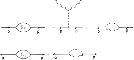
Figure 1: First order corrections to the self energy functions of the interacting Bose gas in the Bogoliubov approximation. Solid lines correspond to propagators of the excited particles, wavy lines to the condensed phase ones. Dashed lines represents the interaction potential. Details of the notation is found in the Appendix.

In this approximation one neglects all of the interactions between the excited atoms, with only those with the condensate taken into account. With this, we may solve (1) and find the propagators as functions of two unknown parameters: the condensed phase density $n_{0}$ and the chemical potential $\mu$. In TFD, one may express any physical parameter of interest via the $G^{11}_{11}$ matrix element of the propagator. In particular, the density $n$ can be written as:

$$n=n_{0}+\int d\omega~{}d\textbf{p}~{}G_{11}^{11}(\omega,\textbf{p};n_{0},\mu)$$ (12)

which gives an implicit dependence of $n_{0}$ on $\mu$. In order to completely characterize the system we also need, therefore, an independent way to determine the chemical potential itself. A common practice here is to use the Hugenholtz-Pines theorem Hugenholtz , which relates this parameter to the self-energy functions of the system Shi ; Andersen . However, we proceed in a different manner and require that the physical values of the condensate density and the chemical potential in a state of equilibrium should minimize the free energy $F$ of the system. In the TFD formalism, interaction corrections to this potential are given by a set of vacuum diagrams in which all internal propagators are of $G^{(0)11}_{11}$ type. As in the case of the self-energy, we maintain only the minimal possible subset of diagrams required, which is depicted in Fig. 2.

Figure 2: First and second order corrections to the free energy of the interacting Bose gas in the Bogoliubov approximation.

Thus, for example, in the first order of approximation the free energy reads:

$$F_{1}=F_{0}-\frac{1}{2}n_{0}(\mu)^{2}U,$$ (13)

where

$$F_{0}=-\frac{kT}{\lambda^{3}}g_{5/2}\left(\exp(\mu)\right)$$ (14)

is the free energy of the ideal Bose gas. Here $k$ is the Boltzmann constant, $T$ is the temperature, $U$ is the interaction potential, $g_{5/2}(x)$ is the Bose-Einstein function Pathria , and $\lambda=h/(2\pi mkT)^{1/2}$ is the thermal wavelength, which, in turn, depends on the mass $m$ of an atom.

In order to keep the procedure consistent, we take into account the interaction corrections to the self- and free energies which are of the same expansion order simultaneously. Our task thus consists of the following steps.

• Given a subset of contributions to the self-energy, we iteratively solve (12) to find $n_{0}$ as a function of $\mu$, $T$ and $n$.

• This value of $n_{0}$ is then used to determine the free energy $F$.

• The chemical potential is adjusted and this process repeated until the minimum of the free energy is found, which thus corresponds to the physical state of equilibrium.

Once the chemical potential and the condensed phase density as functions of temperature are determined, the rest of the parameters of interest follow by applying standard thermodynamic relations.

II.3 Discussion of the method

At first glance, this approach might be seen to suffer from the drawback that the use the Bogoliubov self-energies to explore the thermal properties of the system in a strict perturbative expansion is only accurate in the vicinity of $T=0$. However, the determination within our procedure of the chemical potential involves a partial resummation of terms in the following sense. Let $F_{n}$ be the free energy in the $n$th–order of approximation, given by the sum of the zero order free energy $F_{0}$ and corresponding loop corrections:

$$F_{n}(n_{0},\mu)=F_{0}(n_{0},\mu)+F^{(1)}(n_{0},\mu)+\ldots+F^{(n)}(n_{0},\mu).$$

The chemical potential is determined by minimizing the entire right-hand side of this function, and so places terms of different loop order on the same footing. Thus, a partial mixing of loop order occurs, but the minimization of the free energy makes the outcome of this procedure thermodynamically consistent. The subset of the self–energy diagrams arising in the Bogoliubov approximation is thus regarded as a minimal starting point in this procedure, and we might anticipate this to potentially provide reasonable results at temperatures below the critical temperature. Of course, the ultimate test is to examine the results obtained via this procedure.

II.4 Model parameters

We choose liquid ⁴He as a representative system, and so take the atomic masses and molar volume to be $m=6.65\times 10^{-24}$ g and $V=27.6$ cm³/mole respectively Pathria . Since the momenta involved are sufficiently small due to the low temperature of the system, we assume that the Fourier components of the pair-interaction potential $U(\textbf{p})$ could be replaced by the value $U_{0}$ at $\textbf{p}=0$ Pitaevskii . Thus, the form of the repulsive interaction potential we use is given by

$$U_{0}=\frac{4\pi\hbar^{2}a}{m},$$ (15)

where $a$ is the $s$-wave scattering length. In order to use $U_{0}$ as a loop expansion parameter, the value of $a$ is chosen such that

$$\frac{nU_{0}}{kT_{C}}\approx 0.02,$$ (16)

where $T_{C}\approx 3.13$ K is the critical temperature of the system. In other words, the interaction energy between the particles is assumed to be small compared to the thermal energy. Furthermore, unless otherwise stated, we will assume that the value of $U_{0}$ is unity if it satisfies the assumption of (16).

III Results and discussions

In this Section we present the results of calculations of the first and second order interaction corrections to thermodynamic functions of the ideal Bose gas within this framework.

In Fig. 3 we examine the dependency of the condensate density on temperature in the zeroth, first and second orders of approximation from (12).

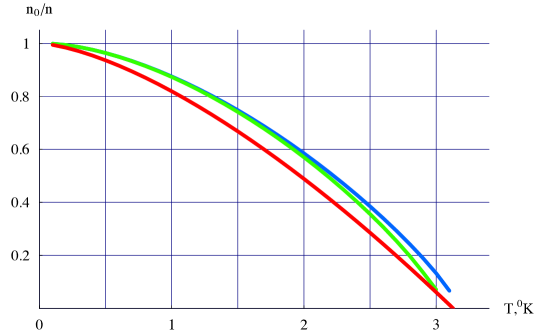
Figure 3: The order parameter as a function of temperature. Red, blue and green lines correspond, respectively, to the zeroth, first and second orders of interaction corrections at unit interaction strength.

Two features of interest are found here. The first is that the second order correction does not alter the overall picture too much compared to the first order one in the whole range of temperatures considered excluding, possibly, the region close to the critical. This is what one expects from higher-order loop corrections, and thus provides a degree of assurance that the perturbative expansion is valid in this region of temperatures. The second feature is that it is difficult to draw any definite conclusions about the system’s properties in the critical region, since the procedure we have followed is not stable there. This is not a reflection of a particular calculational algorithm, but reflects the overall drawback of all theories that try to approach the critical region perturbatively by taking into account only a limited subset of self-energy diagrams into account Andersen ; all such approximations break down near the phase transition due to infrared divergencies. This problem might be cured by a selective resummation of diagrams from all orders of perturbation theory, but since we do not do that here, we cannot make any definite conclusions about the critical region, but rather limit our observations in this region to only general statements.

Thus, we conclude that much of the information concerning the influence of the weak interaction on the order parameter in the whole range of temperatures excluding the critical region is contained already in the first order of approximation. Let us examine this in more detail.

In Fig. 4 the first order interaction correction $n_{01}$ from (12) to the condensed phase density as a function of $T/T_{C}$ is represented for three different values of the interaction strength.

Figure 4: The first order interaction correction to the condensed phase density as a function of $T/T_{C}$. Green, red and blue lines correspond respectively to the interaction parameter $U_{0}$ equal to 1/2, 1 and 2.

First, we notice, that $n_{01}$ is positive everywhere except in a region infinitesimally close to $T=0$. Thus, at very low temperatures the condensed phase density of the weakly interacting Bose gas is lower than that of the ideal gas, even at $T=0$. This effect is a purely entropic nature and appears due to the additional enthalpic term contributed by the interaction. This term increases the entropy, which is physically equivalent to a decrease of the number of condensed particles.

In a strict loop expansion, the region where $n_{01}$ stays negative determines the range of validity of the Bogoliubov approximation. However, as discussed in Section II.3, the partial mixing of loop orders makes possible potential conclusions about the system beyond the scope of the original Bogoliubov construction. Except in an infinitesimal region near $T=0$, the condensed phase density of the interacting gas is higher than of its non–interacting counterpart. An explanation of this could be as follows. The physics of a non-ideal Bose gases is determined by the outcome of the competition between the entropy and enthalpy. While the first favours more particles in a normal phase by increasing the number of accessible microstates as the temperature increases, the second tries to put more atoms into the condensate by the use of repulsive interactions. The point where these two mechanisms balance each other corresponds to the state of thermodynamic equilibrium. The positivity of $n_{01}$ gives us a clue that the interaction term gives a greater contribution to the enthalpy than to the entropy in the whole range of temperatures, starting from the ones just outside of the Bogoliubov domain up to near $T=T_{C}$, where the density correction goes to zero. This seems to imply that the thermal effect is not as significant in an interacting Bose gas as in an ideal gas.

As is clear from Fig. 4, the bigger the interaction strength, the bigger is the $n_{01}$ correction. Qualitatively, this dependency is nonlinear, and two-fold. Firstly, as we observe in Fig. 4, an increase in the magnitude of the interaction is not accompanied by a proportional increase of the value of the correction itself. Secondly, the bigger the value of $U_{0}$, the greater its change impacts $n_{01}$. One may directly observe this effect from the relative distances between the curves while keeping $T/T_{C}$ fixed.

It is also worth noting that the maximum of $n_{01}$ shifts slightly to higher values of temperatures as $U_{0}$ increases. This suggests that the enthalpy is able to dominate the entropy longer the stronger the interaction is between the atoms.

What is also interesting is the absence of a symmetry between the curves with respect to the midpoint $T/T_{C}=1/2$: the bigger the interaction strength, the bigger the asymmetry. As discussed above, this is due to the nonlinear competition between the entropy and enthalpy, which leads to different slopes on the left and right sides of the maximum.

The plot of the dependency of $n_{01}$ on $T/T_{C}$ functionally and on $U_{0}$ parametrically captures most of the physics. We can also extract some limited information about the behaviour of the system as the temperature approaches the critical temperature by examining the first order interaction correction to the specific heat $C_{V1}$ per particle as a function of $T/T_{C}$. This is shown in Fig. 5.

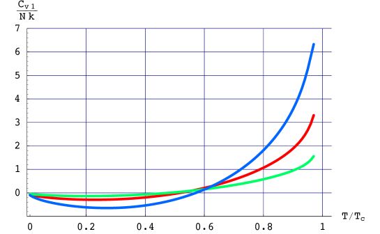
Figure 5: The first order interaction correction to the specific heat per particle as a function of $T/T_{C}$. Green, red and blue lines correspond respectively to the interaction parameter $U_{0}$ equal to 1/2, 1 and 2.

One readily observes the sharp rise of the specific heat as the temperature nears the critical temperature, with the bigger the interaction parameter, the sharper the rise. This is the expected qualitative behaviour of interacting systems near the phase transition point.

One final feature of this approach should be noted. It turns out that in the first order of approximation the chemical potential vanishes. This is in contrast to results obtained within some other approaches where the chemical potential of the ideal Bose gas acquires a small positive correction due to the interaction at first order. In our approach, the second-order correction appears significant in this case, as with this, the chemical potential acquires a small negative value, comparable in order of magnitude with the interaction strength. The magnitude is maximal at $T=0$ and quickly drops to zero in absolute value as the temperature rises, as seen in Fig. 6.

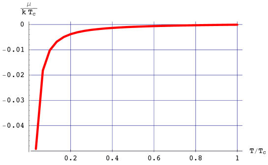
Figure 6: The chemical potential in the second order approximation with unit interaction strength.

This feature of second–order effects being significant when first–order effects vanish is not rare; this is found, for example, in the hard thermal loop resummation of Braaten and Pisarksi pisarski and in certain effective potential calculations involving electroweak interactions carrington .

IV Conclusions

Based on a combination of a loop expansion of the self–energy and a self–consistent minimization of the free energy, we have shown how thermal properties of the weakly interacting Bose gas could be explored within a field theoretic framework. Despite the fact that our procedure uses only the minimal subset of self-energy and free energy contributions, this allows one to evaluate the major effects caused by the interaction already in the leading loop expansion order. A notable feature found is an increase in the condensate density, compared to the non-interacting case, in the whole temperature range excluding a small region near $T=0$, and a sharp rise of the specific heat near the phase transition point. These effects clearly demonstrate that the thermal properties of ideal Bose gases could be changed significantly by the interaction.

However, as with all such perturbative expansions, the physically interesting region near the critical temperature remains inaccessible by our method. Summation to all orders of a broad class of self-energy diagrams is likely required to make reliable conclusions about phenomena taking place near the phase transition point Andersen .

Appendix A The TFD framework

We have chosen the TFD approach as a framework to perform the calculations in this paper due to the physical interpretation possible in a perturbative diagrammatic expansion. Although a doubling of the degrees of freedom is entailed, for lower orders this complication is not extreme, and in any event, physical quantities should be independent of the formalism used to calculate them.

A.1 Formal construction of TFD

The TFD formalism is based on the following arguments Umezawa . Let us imagine an open system, freely exchanging particles and energy with a heat reservoir, maintained at constant inverse temperature $\beta$. The process of annihilation of a quanta of energy $\omega(\textbf{k},\beta)$ in such a system can be regarded as the action of an operator $\alpha(\textbf{k})$ which satisfies the Bose commutation relation:

$$\left[\alpha(\textbf{k}),\alpha^{\dagger}(\textbf{l})\right]=\delta(\textbf{k}-\textbf{l}).$$ (17)

However, unlike the zero temperature case, the operator $\alpha(\textbf{k})$ has an internal structure which incorporates two independent kinds of thermal effects:

• annihilation of a quanta in the system;

• creation of the (Dirac) “holes” maintained by the reservoir;

When the latter process takes place, we say that a $\tilde{\alpha}^{\dagger}$-quantum (hole) with negative energy $-\hbar\omega(\textbf{k})$ and negative momentum $-\hbar\textbf{k}$ is created. The former process will be described by the annihilation operator $\alpha(\textbf{k},\beta)$. Since $\alpha(\textbf{k})$ now performs two independent operations, it can be represented by the linear combination:

$$\alpha(\textbf{k})=c(\textbf{k},\beta)\alpha(\textbf{k},\beta)+d(\textbf{k},\beta)\tilde{\alpha}^{\dagger}(\textbf{k},\beta),$$ (18)

where $c(\textbf{k},\beta)$ and $d(\textbf{k},\beta)$ are certain $c$-number functions. Similarly, the creation operator is

$$\alpha^{\dagger}(\textbf{k})=c^{*}(\textbf{k},\beta)\alpha^{\dagger}(\textbf{k},\beta)+d^{*}(\textbf{k},\beta)\tilde{\alpha}(\textbf{k},\beta),$$ (19)

By construction, the newly introduced temperature dependent operators satisfy Bose commutation relations. This suggests that relations (18-19) could be regarded as a canonical transformation, which implies

$$c(\textbf{k},\beta)c^{*}(\textbf{k},\beta)-d(\textbf{k},\beta)d^{*}(\textbf{k},\beta)=1.$$ (20)

The phase factors of the above coefficients could be absorbed into those of the respective operators, so we can choose $c(\textbf{k},\beta)$ and $d(\textbf{k},\beta)$ to be real.

In order to establish their explicit form, let us use the following considerations. The operator $\alpha^{\dagger}(\textbf{k})$ takes care of the excitations in the system. Therefore, the quantum number density operator is

$$N(\textbf{k})=\alpha^{\dagger}(\textbf{k})\alpha(\textbf{k}).$$ (21)

Since the model we consider is in the grand canonical ensemble, we may require that the vacuum average of this operator should be equal to the corresponding value of the number density in statistical mechanics:

$$n(\textbf{k})=\frac{(2\pi)^{3}}{V}\langle 0,\beta|N(\textbf{k})|0,\beta\rangle=f_{B}(\omega),$$ (22)

with

$$f_{B}(\omega)=\frac{1}{e^{\beta\omega(\textbf{k},\beta)}-1}.$$ (23)

This gives

$$c(\textbf{k},\beta)=\sqrt{1+f_{B}(\omega)},~{}~{}~{}~{}d(\textbf{k},\beta)=\sqrt{f_{B}(\omega)}.$$ (24)

Eq. (22) constitutes the axiom which determines the temperature of the system in a thermal equilibrium state. It can easily be extended to any operator consisting of $\alpha$ and $\alpha^{\dagger}$, say $A(\alpha,\alpha^{\dagger})$. Thus, the vacuum expectation value $\langle 0,\beta|A(\alpha,\alpha^{\dagger})|0,\beta\rangle$ is equal to the ensemble average of $A(\alpha,\alpha^{\dagger})$. In this way, the statistical mechanics of a quantum many-body system becomes a quantum field theory realized in a temperature-dependent Fock space. This formalism is called thermo–field dynamics.

The form of Eqs. (18, 19) suggests that tilde and non-tilde operators are related to each other. Indeed, there is a general TFD “tilde-conjugation” operation which is valid not only for the elementary creation and annihilation operators, but also for arbitrary compound functions $O_{1}$ and $O_{2}$:

$$\widetilde{O_{1}O_{2}}=\tilde{O}_{1}\tilde{O}_{2},$$ (25)

$$\widetilde{c_{1}O_{1}+c_{2}O_{2}}=c^{*}_{1}\tilde{O}_{1}+c^{*}_{2}\tilde{O}_{2},$$ (26)

$$\tilde{\tilde{O}}=O.$$ (27)

Constructing the free TFD Hamiltonian $\hat{H}_{0}$ is now straightforward:

$$\hat{H}_{0}=H_{0}-\tilde{H}_{0}.$$ (28)

with

$$H_{0}=\hbar\int d~{}\textbf{k}~{}\omega(\textbf{k})\alpha^{\dagger}(\textbf{k},\beta)\alpha(\textbf{k},\beta),~{}~{}~{}\tilde{H}_{0}=\hbar\int d~{}\textbf{k}~{}\omega(\textbf{k})\tilde{\alpha}^{\dagger}(\textbf{k},\beta)\tilde{\alpha}(\textbf{k},\beta)$$ (29)

or, equivalently, with the use of the canonical transformation

$$H_{0}=\hbar\int d~{}\textbf{k}~{}\omega(\textbf{k})\alpha^{\dagger}(\textbf{k})\alpha(\textbf{k}),~{}~{}~{}\tilde{H}_{0}=\hbar\int d~{}\textbf{k}~{}\omega(\textbf{k})\tilde{\alpha}^{\dagger}(\textbf{k})\tilde{\alpha}(\textbf{k}).$$ (30)

A.2 Green’s functions in TFD

Let us now consider the simple example of a free field at finite temperature. Suppose such a field $\phi^{0}$ satisfies the equation $\lambda(\partial)\phi^{0}=0$, with

$$\lambda(\partial)=i\frac{\partial}{\partial t}-\omega(\nabla).$$ (31)

The expressions for the tilde- and non-tilde Hamiltonians read:

$$H_{0}=\int d\textbf{x}\ \phi^{0\dagger}\omega(\nabla)\phi^{0},$$ (32)

$$\tilde{H}_{0}=\int d\textbf{x}\ \tilde{\phi}^{0\dagger}\omega(-\nabla)\tilde{\phi}^{0},$$ (33)

where the relation $\omega^{*}(\nabla)=\omega(-\nabla)$ from the tilde-conjugation rules (25-27) has been used. The corresponding equations of motion

$$i\hbar\frac{\partial}{\partial t}\phi^{0}(\textbf{x})=\left[\phi^{0}(\textbf{x}),H_{0}\right],$$ (34)

$$i\hbar\frac{\partial}{\partial t}\tilde{\phi}^{0}(\textbf{x})=-\left[\tilde{\phi}^{0}(\textbf{x}),\tilde{H}_{0}\right].$$ (35)

have the formal solution:

$$\phi^{0}(\textbf{x})=\frac{\sqrt{\hbar}}{(2\pi)^{3/2}}\int d\textbf{k}\ \alpha(\textbf{k})\exp[i\textbf{k}\cdot\textbf{x}-i\omega(\textbf{k})t],$$ (36)

$$\tilde{\phi}^{0}(\textbf{x})=\frac{\sqrt{\hbar}}{(2\pi)^{3/2}}\int d\textbf{k}\ \tilde{\alpha}(\textbf{k})\exp[-i\textbf{k}\cdot\textbf{x}+i\omega(\textbf{k})t].$$ (37)

It is useful to simplify the notation by introducing the following thermal doublet symbol:

$$\left(\begin{array}[]{ccc}\phi^{1}\\ \phi^{2}\end{array}\right)=\left(\begin{array}[]{ccc}\phi^{0}\\ \tilde{\phi}^{0\dagger}\end{array}\right).$$ (38)

The causal two-point function is then defined by

$$G^{(0)\alpha\beta}(x-y) = \langle 0,\beta|T[\phi^{\alpha}(x),\phi^{\beta\dagger}(y)]|0,\beta\rangle=$$

$$= \theta(t_{x}-t_{y})\langle 0,\beta|\phi^{\alpha}(x)\phi^{\beta\dagger}|0,\beta\rangle+\theta(t_{y}-t_{x})\langle 0,\beta|\phi^{\beta\dagger}(y)\phi^{\alpha}(x)|0,\beta\rangle$$ (39)

where the symbol $T$ denotes ordering along the TFD time contour in the complex plane semenoff , and the average is over the temperature-dependent vacuum. Using (36, 37) and the canonical transformations (18, 19), we find that in the momentum representation the above function reads:

$$G^{(0)\alpha\beta}(k_{0},\textbf{k}) = \left(\begin{array}[]{ll}{\displaystyle\frac{c^{2}_{B}(\omega)}{k_{0}-\omega+i\epsilon}-\frac{d^{2}_{B}(\omega)}{k_{0}-\omega-i\epsilon}}&{\displaystyle\frac{c_{B}(\omega)d_{B}(\omega)}{k_{0}-\omega+i\epsilon}-\frac{c_{B}(\omega)d_{B}(\omega)}{k_{0}-\omega-i\epsilon}}\\ &\\ {\displaystyle\frac{c_{B}(\omega)d_{B}(\omega)}{k_{0}-\omega+i\epsilon}-\frac{c_{B}(\omega)d_{B}(\omega)}{k_{0}-\omega-i\epsilon}}&{\displaystyle\frac{d^{2}_{B}(\omega)}{k_{0}-\omega+i\epsilon}-\frac{c^{2}_{B}(\omega)}{k_{0}-\omega-i\epsilon}}\end{array}\right)$$ (43)

where $\omega=\omega(\textbf{k})$ and $c_{B}(\omega),d_{B}(\omega)$ are given by (22). This free propagator (43) is the building block for the development of perturbation theory, which we now discuss.

A.3 Feynman diagrams in TFD

Perturbative calculations in TFD are similar to those at zero temperature, and indeed, one of the virtues of the formalism is that the machinery of renormalization and the renormalization group equations are readily incorporated. The doubling of degrees of freedom discussed above leads to a $2\times 2$ matrix structure of propagators and self energies. This feature implies that in higher orders a much larger number of diagrams has to be taken into account, compared to the vacuum theory, and calculations may become cumbersome. However, for calculations to low orders, this is not a serious problem.

In general, Feynman diagrams turn out to be topologically and combinatorically identical to those of the corresponding zero-temperature quantum field theory, but generalized to a two-component formalism. The first (type 1) component represents, by construction, the “physical” field, describing propagation of excitations in the system. The second (type 2) component corresponds to a “thermal ghost field”, corresponding to holes, maintained by the reservoir. In TFD, two types of vertices occur: one type describing the interactions of the type 1 fields, and the other of the type 2 fields. The Feynman rules for these two types of fields differ only by a sign in the case of even interactions. There is no direct coupling between the two types of fields, but they can propagate into each other because of the non-diagonal 1–2 and 2–1 elements of the propagator matrix. The 1–1 and 2–2 components correspond to physical and ghost propagators. Therefore, external lines of physical Green’s function are always of type 1. In order to find a particular $n$-point Green’s function in momentum space, one must draw all topologically distinct diagrams with $n$ external points of type 1, and then sum over internal vertices of types 1 and 2. The ultimate goal is to compute the 1–1 matrix component of the Green’s function, which can then be used to calculate physical quantities of interest.

A.4 Weakly interacting Bose gas in TFD

Let us now formulate the general problem of a weakly interacting Bose gas within the TFD framework.

The system we study is a dilute gas consisting of $N$ atoms obeying Bose statistics, enclosed in a box of volume $V$ and interacting through a two-body potential $U(\textbf{x}-\textbf{y})$. The interaction is assumed to be weak which, together with the low density of the gas, allows us to neglect higher-order interactions and treat the system’s properties perturbatively. For simplicity, the atoms are assumed to have zero net spin, and are described by the boson field operators $\psi(\textbf{x}),\psi^{\dagger}(\textbf{x})$ subject to the Bose commutation relations:

$$[\psi(\textbf{x}),\psi(\textbf{y})]=0,$$ (44)

$$[\psi^{\dagger}(\textbf{x}),\psi^{\dagger}(\textbf{y})]=0,$$ (45)

$$[\psi(\textbf{x}),\psi^{\dagger}(\textbf{y})]=\delta(\textbf{x}-\textbf{y})$$ (46)

The system is immersed in a large heat reservoir, with which it can freely exchange both energy and particles. In a state of equilibrium both the system and the reservoir possess the same chemical potential $\mu$ and inverse temperature $\beta$. In TFD it is assumed that the reservoir, unlike the system, maintains the negative-energy holes, represented by the operators obtained by the tilde-conjugation operation of (25-27). They satisfy the same commutation relations as the regular operators, while all commutators between the tilde- and non-tilde operators vanishing by construction.

In equilibrium, the system contains a mixture of particles and holes. Therefore, its Hamiltonian $\hat{H}$ is given by

$$\hat{H}=K-\tilde{K},$$ (47)

where

$$K=H_{0}-\mu N = \int d\textbf{x}\ \psi^{\dagger}(\textbf{x})\left[-\frac{\hbar^{2}}{2m}\nabla^{2}-\mu\right]\psi(\textbf{x})$$

$$+ \frac{1}{2}\int d\textbf{x}\int d\textbf{y}\psi^{\dagger}(\textbf{x})\psi^{\dagger}(\textbf{y})U(\textbf{x}-\textbf{y})\psi(\textbf{y})\psi(\textbf{x})$$

is the regular zero-temperature Hamiltonian describing the particles of the system and $\tilde{K}$ is its tilde-conjugate, describing the holes:

$$\tilde{K}=\tilde{H_{0}}-\mu\tilde{N} = \int d\textbf{x}\ \tilde{\psi}^{\dagger}(\textbf{x})\left[-\frac{\hbar^{2}}{2m}\nabla^{2}-\mu\right]\tilde{\psi}(\textbf{x})$$

$$+ \frac{1}{2}\int d\textbf{x}\int d\textbf{y}\tilde{\psi}^{\dagger}(\textbf{x})\tilde{\psi}^{\dagger}(\textbf{y})U(\textbf{x}-\textbf{y})\tilde{\psi}(\textbf{y})\tilde{\psi}(\textbf{x}).$$

The chemical potential $\mu$ is chosen such that the vacuum average of the atomic number operator is equal to the total number of particles in the system:

$$\langle\hat{N}\rangle=N.$$ (50)

With the Hamiltonian $\hat{H}$, one may introduce the time-dependent Heisenberg picture for any Schrödinger operator $O(\textbf{x})$ and its tilde-conjugate $\tilde{O}(\textbf{x})$:

$$O(\textbf{x},t) \equiv e^{iKt}O(\textbf{x})e^{-iKt},$$ (51)

$$\tilde{O}(\textbf{x},t) \equiv e^{-i\tilde{K}t}\tilde{O}(\textbf{x})e^{i\tilde{K}t}.$$ (52)

In particular, the field operators have a time-dependence given by

$$\psi(\textbf{x},t) = e^{iKt}\psi(\textbf{x})e^{-iKt},$$ (53)

$$\psi^{\dagger}(\textbf{x},t) = e^{-iKt}\psi^{\dagger}(\textbf{x})e^{iKt};$$ (54)

$$\tilde{\psi}(\textbf{x},t) = e^{-i\tilde{K}t}\tilde{\psi}(\textbf{x})e^{i\tilde{K}t},$$ (55)

$$\tilde{\psi}^{\dagger}(\textbf{x},t) = e^{i\tilde{K}t}\tilde{\psi}^{\dagger}(\textbf{x})e^{-i\tilde{K}t}.$$ (56)

In order to simplify the notation, we introduce the thermal doublet symbol (see (38))

$$\left(\begin{array}[]{ccc}\psi^{1}(\textbf{x},t)\\ \psi^{2}(\textbf{x},t)\end{array}\right)=\left(\begin{array}[]{ccc}\psi(\textbf{x},t)\\ \tilde{\psi}^{\dagger}(\textbf{x},t)\end{array}\right).$$ (57)

The single-particle Green’s function is then defined as:

$$G^{\alpha\beta}(\textbf{x},t;\textbf{x}^{\prime},t^{\prime})=\langle 0,\beta|T[\psi^{\alpha}(\textbf{x},t),\psi^{\beta\dagger}(\textbf{x}^{\prime},t^{\prime})]|0,\beta\rangle,$$ (58)

For our purposes, it is more convenient to work in the single-particle momentum representation. In this representation, the field operators $\psi(\textbf{x}),\tilde{\psi}(\textbf{x})$ can be written as

$$\psi(\textbf{x})=\frac{1}{(2\pi)^{3/2}}\int d\textbf{k}\ a_{\textbf{k}}\phi_{\textbf{k}}(\textbf{x}),$$ (59)

$$\tilde{\psi}(\textbf{x})=\frac{1}{(2\pi)^{3/2}}\int d\textbf{k}\ \tilde{a}_{\textbf{k}}\tilde{\phi}_{\textbf{k}}(\textbf{x}),$$ (60)

where $a_{\textbf{k}}(a^{\dagger}_{\textbf{k}})$ and $\tilde{a}_{\textbf{k}}(\tilde{a}^{\dagger}_{\textbf{k}})$ are the creation (annihilation) operators for a particle and hole in single-particle states $\phi_{\textbf{k}}(\textbf{x})$ and $\tilde{\phi}_{\textbf{k}}(\textbf{x})$, respectively. These obey Bose commutation relations:

$$[a_{\textbf{k}},\ a_{\textbf{k}^{\prime}}]=0,\ \ \ [a_{\textbf{k}},\ a_{\textbf{k}^{\prime}}^{\dagger}]=\delta_{\textbf{k},\textbf{k}^{\prime}};$$ (61)

$$[\tilde{a}_{\textbf{k}},\ \tilde{a}_{\textbf{k}^{\prime}}]=0,\ \ \ [\tilde{a}_{\textbf{k}},\ \tilde{a}^{\dagger}_{\textbf{k}^{\prime}}]=\delta_{\textbf{k},\textbf{k}^{\prime}},$$ (62)

with all commutators between the tilde and non-tilde operators vanishing.

Just as in the case of fields, we may introduce the thermal doublet notation for the operators $a_{\textbf{k}}$ and $\tilde{a}_{\textbf{k}}$ and then write the Green’s function $G^{\alpha\beta}(\textbf{x},t;\textbf{x}^{\prime},t^{\prime})$ in the single-particle momentum representation as

$$G^{\alpha\beta}(\textbf{x},t;\textbf{x}^{\prime},t^{\prime})=\frac{1}{(2\pi)^{3}}\int d\textbf{k}\int d\textbf{k}^{\prime}\phi_{\textbf{k}}^{\alpha}(\textbf{x}){\phi}_{\textbf{k}^{\prime}}^{\beta\dagger}(\textbf{x}^{\prime})\langle 0,\beta|T[a_{\textbf{k}}^{\alpha}(t),a_{\textbf{k}^{\prime}}^{\beta\dagger}(t^{\prime})]|0,\beta\rangle.$$ (63)

In the case of a uniform system governed by a time-independent Hamiltonian, the single-particle states are plane waves

$$\phi_{\textbf{k}}(\textbf{x}) = \frac{1}{\sqrt{V}}\exp(i\textbf{k}\cdot\textbf{r}),$$ (64)

$$\tilde{\phi}_{\textbf{k}}(\textbf{x}) = \frac{1}{\sqrt{V}}\exp(-i\textbf{k}\cdot\textbf{r}).$$ (65)

Similarly, $G^{\alpha\beta}(\textbf{x},t;\textbf{x}^{\prime},t^{\prime})$ now depends only on the differences $\textbf{x}-\textbf{x}^{\prime}$ and $t-t^{\prime}$, so that

$$G^{\alpha\beta}(\textbf{x},t)=\int d\textbf{k}\ e^{i\textbf{k}\cdot\textbf{x}}G^{\alpha\beta}(\textbf{k},t),$$ (66)

where

$$G^{\alpha\beta}(\textbf{k},t)\equiv\langle 0,\beta|T[a_{\textbf{k}}^{\alpha}(t),a_{\textbf{k}}^{\beta\dagger}(0)]0,\beta\rangle$$ (67)

is the single-particle Green’s function in the momentum representation.

The remaining task is to calculate the Green’s function $G^{\alpha\beta}(\textbf{k},t)$. For a system of Bose particles, this task is complicated by the possible phase transition to a Bose-condensed state by spontaneous symmetry breaking below a certain critical temperature $T_{C}$. This is signalled by a non-vanishing average

$$\langle 0,\beta|\psi^{\alpha}(\textbf{x})|0,\beta\rangle\equiv\Phi_{0}^{\alpha}(\textbf{x})\neq 0,$$ (68)

The function $\Phi_{0}^{\alpha}(\textbf{x})$ is often referred to as the macroscopic wave function of the condensate and in general has an amplitude and phase. In a uniform system and in the absence of any supercurrent, we can take $\Phi_{0}^{\alpha}(\textbf{x})$ to be real and independent of position. In this case, $\Phi_{0}^{\alpha}(\textbf{x})$ is equal to the square root of the condensate density $n_{0}$. We are then led to separate the boson field operator $\psi^{\alpha}(\textbf{x})$ into two parts:

$$\psi^{\alpha}(\textbf{x})\equiv a^{\alpha}_{0}/V^{1/2}+\bar{\psi}^{\alpha}(\textbf{x}),$$ (69)

$$\psi^{\alpha\dagger}(\textbf{x})\equiv a^{\alpha\dagger}_{0}/V^{1/2}+\bar{\psi}^{\alpha\dagger}(\textbf{x}).$$ (70)

The commutator of $a_{0}^{\alpha}$ and $a_{0}^{\alpha\dagger}$ is unity, while their product is of order $N$. Therefore, we may neglect the operator nature of $a_{0}^{\alpha}$ and $a_{0}^{\alpha\dagger}$ and replace them by the $c$-number $\sqrt{N_{0}}$. This procedure, known as the Bogoliubov prescription, is appropriate when the number of particles in the zero-momentum state is a finite fraction of $N$. The error thus introduced is of the order $O(V^{-1})$ and vanishes in the thermodynamic limit. The new field operators $\bar{\psi}^{\alpha}(\textbf{x}),\bar{\psi}^{\alpha\dagger}(\textbf{x})$ describe the normal phase atoms, satisfy Bose commutation relations, and have vanishing vacuum averages:

$$\langle 0,\beta|\bar{\psi}^{\alpha}(\textbf{x})|0,\beta\rangle=\langle 0,\beta|\bar{\psi}^{\alpha\dagger}(\textbf{x})|0,\beta\rangle=0.$$ (71)

With this, the thermal Green’s function now becomes:

$$G^{\alpha\beta}(\textbf{x},t;\textbf{x}^{\prime},t^{\prime})=-n_{0}+\bar{G}^{\alpha\beta}(\textbf{x},t;\textbf{x}^{\prime},t^{\prime}),$$ (72)

where $\bar{G}^{\alpha\beta}(\textbf{x},t;\textbf{x}^{\prime},t^{\prime})$ is its non-condensate part defined by

$$\bar{G}^{\alpha\beta}(\textbf{x},t;\textbf{x}^{\prime},t^{\prime})\equiv-\langle 0,\beta|T[\bar{\psi}^{\alpha}(\textbf{x},t),\bar{\psi}^{\beta\dagger}(\textbf{x}^{\prime},t^{\prime})]|0,\beta\rangle.$$ (73)

In the momentum representation for $\textbf{k}\neq 0$, we have

$$\bar{G}^{\alpha\beta}(\textbf{k},t)=-\langle 0,\beta|T[a_{\textbf{k}}^{\alpha}(t),a_{\textbf{k}}^{\beta\dagger}(0)]|0,\beta\rangle.$$ (74)

The Bogoliubov prescription modifies the Hamiltonian (47) in a fundamental way. In order to simplify matters, we will concentrate on the zero-temperature part $K$ for the moment, making a straightforward generalization to TFD later on. After all of the above transformations, $K$ reads

$$K=E_{0}-\mu N_{0}+\frac{1}{V}\sum_{\textbf{k}\neq 0}(\varepsilon_{\textbf{k}}-\mu)a_{\textbf{k}}^{\dagger}a_{\textbf{k}}+\sum_{j=1}^{7}\hat{V}_{j},$$ (75)

where the interaction term $\hat{V}$ can be separated into the following eight distinct parts:

$$E_{0}=\frac{1}{2}n_{0}^{2}VU(0),$$ (76)

$$\hat{V}_{1}=\frac{1}{2}n_{0}\sum_{\textbf{k}}U(\textbf{k})a_{\textbf{k}}a_{-\textbf{k}},$$ (77)

$$\hat{V}_{2}=\frac{1}{2}n_{0}\sum_{\textbf{k}}U(\textbf{k})a^{\dagger}_{\textbf{k}}a_{-\textbf{k}},$$ (78)

$$\hat{V}_{3}=n_{0}\sum_{\textbf{k}}U(\textbf{k})a_{\textbf{k}}^{\dagger}a_{\textbf{k}},$$ (79)

$$\hat{V}_{4}=n_{0}\sum_{\textbf{k}}U(\textbf{0})a_{\textbf{k}}^{\dagger}a_{\textbf{k}},$$ (80)

$$\hat{V}_{5}=\frac{n_{0}^{1/2}}{V^{1/2}}\sum_{\textbf{k},\textbf{q}}U(\textbf{q})a_{\textbf{k}+\textbf{q}}a_{\textbf{k}}a_{\textbf{q}},$$ (81)

$$\hat{V}_{6}=\frac{n_{0}^{1/2}}{V^{1/2}}\sum_{\textbf{k},\textbf{q}}U(\textbf{q})a_{\textbf{k}}^{\dagger}a_{\textbf{q}}^{\dagger}a_{\textbf{k}+\textbf{q}},$$ (82)

$$\hat{V}_{7}=\frac{1}{2V}\sum_{\textbf{k},\textbf{k}^{\prime},\textbf{q}}U(\textbf{q})a_{\textbf{k}+\textbf{q}}^{\dagger}a_{\textbf{k}^{\prime}-\textbf{q}}^{\dagger}a_{\textbf{k}^{\prime}}a_{\textbf{k}}$$ (83)

with

$$U(\textbf{q})\equiv\int d\textbf{x}\ e^{i\textbf{q}\cdot\textbf{x}}U(\textbf{x}).$$ (84)

In a normal system ($n_{0}=0$), only $\hat{V}_{7}$ is present. We also note that $K$ has no term containing a single $a_{\textbf{k}}^{\dagger}$ or $a_{\textbf{k}}$ because these would violate momentum conservation. This is in agreement with (71), which gives in a momentum representation

$$\langle 0,\beta|a_{\textbf{k}}|0,\beta\rangle=\langle 0,\beta|a_{\textbf{k}}^{\dagger}|0,\beta\rangle=0,\ \ \ (\textbf{k}\neq 0).$$ (85)

The fact that there exist interaction terms such as $\hat{V}_{1}$ implies the non-conservation of particles in the system described by non–condensate operators $a_{\textbf{k}}$ and $a_{\textbf{k}}^{\dagger}$ due to exchanges between non-condensate atoms and the condensate atoms. This changes the way the proper self-energies are defined. There are three distinct types of them now, indicated in Fig. 7.

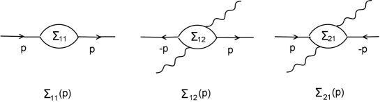
Figure 7: Proper self-energies for a Bose-condensed system. Straight lines correspond to the normal phase particles, with wavy lines associated with the condensed phase.

For $\Sigma_{11}$ there is one particle line coming in and one coming out. The others components have two particle lines either coming out $(\Sigma_{12})$ or going in $(\Sigma_{21})$, and reflect the new features associated with the existence of a Bose condensate. We then introduce two new Green’s functions:

$$G_{12}(\textbf{k},t)\equiv-\langle 0,\beta|Ta_{-\textbf{k}}(t)a_{\textbf{k}}(0)|0,\beta\rangle,$$ (86)

$$G_{21}(\textbf{k},t)\equiv-\langle 0,\beta|Ta_{\textbf{k}}^{\dagger}(t)a_{-\textbf{k}}^{\dagger}(0)|0,\beta\rangle.$$ (87)

The functions $G_{12}$ and $G_{21}$ are usually called “anomalous” Green’s functions, representing the disappearance and appearance of two non-condensate particles, respectively. The normal Green’s function is denoted as $G_{11}$ and represents the propagation of a single particle

$$G_{11}(\textbf{k},t)\equiv-\langle 0,\beta|Ta_{\textbf{k}}(t)a_{\textbf{k}}^{\dagger}(0)|0,\beta\rangle.$$ (88)

These three Green’s functions are shown in Fig. 8, where the arrows indicate the direction of momentum of the atoms involved.

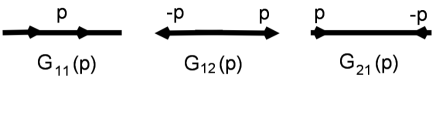
Figure 8: Green’s functions for a Bose-condensed system.

The Dyson equations connecting the above free energies and propagators is found in standard textbooks. For the case of zero-temperature Beliaev , they where first written down by Beliaev, and are illustrated diagrammatically in Fig. 9.

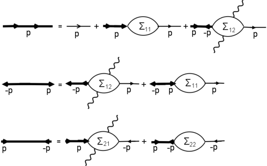
Figure 9: The Dyson-Beliaev equations for a Bose-condensed system. Thin and thick straight lines denote, respectively, the free and full propagators of the normal phase particles.

The generalization of this to TFD is straightforward and in the momentum representation reads:

$$G_{11}^{\alpha\beta}(p)=G^{(0)\alpha\beta}(p)+G_{11}^{\alpha\gamma}(p)\Sigma_{11}^{\gamma\delta}(p)G^{(0)\delta\beta}(p)+G_{21}^{\alpha\gamma}(p)\Sigma_{12}^{\gamma\delta}(p)G^{(0)\delta\beta}(p),$$ (89)

$$G_{12}^{\alpha\beta}(p)=G_{11}^{\alpha\gamma}(-p)\Sigma_{12}^{\gamma\delta}(p)G^{(0)\delta\beta}(p)+G_{12}^{\alpha\gamma}(p)\Sigma_{11}^{\gamma\delta}(p)G^{(0)\delta\beta}(p),$$ (90)

$$G_{21}^{\alpha\beta}(p)=G_{11}^{\alpha\gamma}(p)\Sigma_{21}^{\gamma\delta}(p)G^{(0)\delta\beta}(-p)+G_{21}^{\alpha\gamma}(p)\Sigma_{22}^{\gamma\delta}(-p)G^{(0)\delta\beta}(p).$$ (91)

Here the TFD indices $\alpha,\beta$ take the values of 1 and 2 and summation over repeated indices is implied. The notation $p=(p_{0},\textbf{p})$ is employed and the expression for the unperturbed Green’s function $G^{(0)\alpha\beta}(p)$ is given by (43). There are some useful relations between the anomalous proper self-energies and propagators:

$$G_{12}^{\alpha\beta}(p)=G_{21}^{\alpha\beta}(-p),~{}~{}~{}G_{22}^{\alpha\beta}(p)=G_{11}^{\alpha\beta}(-p),~{}~{}~{}\Sigma_{12}^{\alpha\beta}(p)=\Sigma_{21}^{\alpha\beta}(-p),~{}~{}~{}\Sigma_{22}^{\alpha\beta}(p)=\Sigma_{11}^{\alpha\beta}(-p)$$ (92)

Eqs. (89-91) could be solved with respect to the propagators in terms of the exact proper self-energies and unperturbed Green’s functions. Therefore, they are completely general and can be applied to any uniform Bose-condensed fluid, liquid or gas, without any reference to whether the underlying system is weakly interacting or not. However, except in special cases, a closed–form solution is generally not possible, which leads to consideration of various approximation schemes. Many such schemes, including ours, use Eqs. (89-91) as a starting point.

- (1) M. H. Anderson, J. R. Ensher, M. R. Matthews, C. Wieman, and E. A. Cornell, Science 269, 198 (1995).
- (2) C. C. Bradley, C. A. Sackett, J. J. Tollett, and R. G. Hulet, Phys. Rev. Lett. 75, 1687 (1995).
- (3) K. B. Davis, M. O. Mewes, M. R. Andrews, N. J. van Druten, D. S. Durfee, D. M. Kurn, and W. Ketterle, Phys. Rev Lett. 75, 3969 (1995).
- (4) H. Shi and A. Griffin, Phys. Rep. 304, 1 (1998).
- (5) L. P. Pitaevskii and S. Stringari, Bose-Einstein condensation, Oxford University Press (2003).
- (6) J. O. Andersen, Rev. Mod. Phys. 76, 599 (2004).
- (7) T. Haugset, H. Haugerud and F. Ravndal, Ann. Phys. (N. Y. ) 266, 27 (1998).
- (8) D. J. Toms, Phys. Rev. A66, 013619 (2002).
- (9) M. B. Pinto, R. O. Ramos and F. F. de Souza Cruz, Phys. Rev. A74, 033618 (2006).
- (10) Zeng-Qiang Yu and Lan Yin, Phys. Rev. A81, 023613 (2010).
- (11) Nick P. Proukakis and Brian Jackson, Phys. B: At. Mol. Opt. Phys. 41, 203002 (2008).
- (12) H. Umezawa, Thermo Field Dynamics and Condensed States, Elsevier Science Ltd (1982).
- (13) N. P. Landsman and Ch. G. van Weert, Phys. Rep. 145, 141 (1987).
- (14) J. I. Kapusta, Finite Temperature Field Theory (Cambridge University Press, Cambridge, England, 1989).
- (15) M. LeBellac, Thermal Field Theory (Cambridge University Press, Cambridge, England, 1996).
- (16) A. J. Niemi and G. W. Semenoff, Annals Phys. 152, 105 (1984).
- (17) E. M. Lifshits and L. P. Pitaevskii, Statistical physics, Volume 9, Butterworth-Heinemann (1980).
- (18) A. A. Abrikosov, Methods of Quantum Field Theory in Statistical Physics, Dover Publications (1975).
- (19) N. N. Bogoliubov, J. Phys. U. S. S. R. 23, 11 (1947).
- (20) S. T. Beliaev, Soviet Phys. JETP 7, 289 (1958).
- (21) A. Griffin, Excitations in a Bose-condensed Liquid, Cambridge University Press (1993).
- (22) R. K. Pathria, Statistical mechanics, Butterwotrth-Heinemann (2003).
- (23) N. M. Hugenholtz and D. Pines, Phys. Rev. 116, 489 (1959).
- (24) E. Braaten and R. D. Pisarski, Nucl. Phys. B334, 199 (1990).
- (25) M. E. Carrington, Phys. Rev. D45, 2993 (1992).