An Optimal Linear Time Algorithm for Quasi-Monotonic Segmentation

Abstract

Monotonicity is a simple yet significant qualitative characteristic. We consider the problem of segmenting a sequence in up to $K$ segments. We want segments to be as monotonic as possible and to alternate signs. We propose a quality metric for this problem using the $l_{\infty}$ norm, and we present an optimal linear time algorithm based on novel formalism. Moreover, given a precomputation in time $O(n\log n)$ consisting of a labeling of all extrema, we compute any optimal segmentation in constant time. We compare experimentally its performance to two piecewise linear segmentation heuristics (top-down and bottom-up). We show that our algorithm is faster and more accurate. Applications include pattern recognition and qualitative modeling.

H.2.8

1 Introduction

Monotonicity is one of the most natural and important qualitative properties for sequences of data points. It is easy to determine where the values are strictly going up or down, but we only want to identify significant monotonicity. For example, the drop from 2 to 1.9 in the array $0,1,2,1.9,3,4$ might not be significant and might even be noise-related. The quasi-monotonic segmentation problem is to determine where the data is approximately increasing or decreasing.

In practical applications, sequences of values can be quite large: it is not uncommon to have sensors record data at 10 kHz or more, thus generating terabytes of data and billions of data points. As a dimensionality reduction step [2], segmentation divides the data into intervals having homogeneous characteristics (flatness, constant slope [3], unimodality [4], monotonicity [5, 6], step, ramp or impulse [7], and so on). The segmentation points can also be used as markers to indicate a qualitative change in the data. Other applications include frequent pattern mining [8] and time series classification [9]. For qualitative reasoning [10], piecewise monotonic segmentation is especially important as it provides a symbolic model describing system behavior in terms of increasing and decreasing relations between variables.

There is a trade-off between the number of segments and the approximation error. Some segmentation algorithms [5] give a segmentation having no more than $K$ segments while attempting to minimize the error $\epsilon$; other algorithms [6] attempt to minimize the number of segments ($K$) given an upper bound on the error $\epsilon$. We are concerned with the first type of algorithm in this paper.

Using dynamic programming or other approaches, most segmentation problems can be solved in time $O(n^{2})$. Other solutions to this problem, using machine learning to classify the pairs of data points [10], are even less favorable since they have higher complexity. However, it is common for sequence of data points to be massive and segmentation algorithms have to have complexity close to $O(n)$ to be competitive. While approximate linear regression segmentation algorithms can be $O(n)$, we show that using a linear regression error to segment according to monotonicity is not an ideal solution.

We present a metric for the quasi-monotonic segmentation problem called the Optimal Monotonic Approximation Function Error (OMAFE); this metric differs from previously introduced OPMAFE metric [5] since it applies to all segmentations and not just “extremal” segmentations. We formalize the novel concept of a maximal $\ast$-pair and shows that it can be used to define a unique labeling of the extrema leading to an optimal segmentation algorithm. We also present an optimal linear time algorithm to solve the quasi-monotonic segmentation problem given a segment budget together with an experimental comparison to quantify the benefits of our algorithm.

2 Monotonicity Error Metric (OMAFE)

Finding the best piecewise monotonic approximation can be viewed as a classical functional approximation problem [11], but we are concerned only with discrete sequences.

Suppose $n$ samples noted $F:D=\{x_{1},\ldots,x_{n}\}\rightarrow\mathbb{R}$ with $x_{1}<x_{2}<\ldots x_{n}$. We define, $F_{|[a,b]}$ as the restriction of $F$ over $D\cap[a,b]$. We seek the best monotonic (increasing or decreasing) function $f:\mathbb{R}\rightarrow\mathbb{R}$ approximating $F$. Let $\Omega_{\uparrow}$ (resp. $\Omega_{\downarrow}$) be the set of all monotonic increasing (resp. decreasing) functions. The Optimal Monotonic Approximation Function Error (OMAFE) is $\min_{f\in\Omega}\max_{x\in D}|f(x)-F(x)|$ where $\Omega$ is either $\Omega_{\uparrow}$ or $\Omega_{\downarrow}$.

The segmentation of a set $D$ is a sequence $S=X_{1},\dots,X_{K}$ of intervals in $\mathbb{R}$ with $[\min D,\max D]=\bigcup_{i}X_{i}$ such that $\max X_{i}=\min X_{i+1}\in D$ and $X_{i}\cap X_{j}=\emptyset$ for $j\neq i+1,i,i-1$. Alternatively, we can define a segmentation from the set of points $X_{i}\cap X_{i+1}=\{y_{i+1}\}$, $y_{1}=\min X_{1}$, and $y_{K+1}=\max X_{K}$. Given $F:\{x_{1},\ldots,x_{n}\}\rightarrow\mathbb{R}$ and a segmentation, the Optimal Monotonic Approximation Function Error (OMAFE) of the segmentation is $\max_{i}\textrm{OMAFE}(F_{|X_{i}})$ where the monotonicity type (increasing or decreasing) of the segment $X_{i}$ is determined by the sign of $F(\max X_{i})-F(\min X_{i})$. Whenever $F(\max X_{i})=F(\min X_{i})$, we say the segment has no direction and the best monotonic approximation is just the flat function having value $(\max F_{|X_{i}}-\min F_{|X_{i}})/2$. The error is computed over each interval independently; optimal monotonic approximation functions are not required to agree at $\max X_{i}=\min X_{i+1}$. Segmentations should alternate between increasing and decreasing, otherwise sequences such as $0,2,1,0,2$ can be segmented as two increasing segments $0,2,1$ and $1,0,2$: we consider it is natural to aggregate segments with the same monotonicity.

We solve for the best monotonic function as follows. If we seek the best monotonic increasing function, we first define $\overline{f}_{\uparrow}(x)=\max\{F(y):y\leq x\}$ (the maximum of all previous values) and $\underline{f}_{\uparrow}(x)=\min\{F(y):y\geq x\}$ (the minimum of all values to come). If we seek the best monotonic decreasing function, we define $\overline{f}_{\downarrow}(x)=\max\{F(y):y\geq x\}$ (the maximum of all values to come) and $\underline{f}_{\downarrow}(x)=\min\{F(y):y\leq x\}$ (the minimum of all previous values). These functions, which can be computed in linear time, are all we need to solve for the best approximation function as shown by the next theorem which is a well-known result [12].

Theorem 2.1.

Given $F:D=\{x_{1},\ldots,x_{n}\}\rightarrow\mathbb{R}$, a best monotonic increasing approximation function to $F$ is $f_{\uparrow}=(\overline{f}_{\uparrow}+\underline{f}_{\uparrow})/2$ and a best monotonic decreasing approximation function is $f_{\downarrow}=(\overline{f}_{\downarrow}+\underline{f}_{\downarrow})/2$. The corresponding error (OMAFE) is $\max_{x\in D}(|\overline{f}_{\uparrow}(x)-\underline{f}_{\uparrow}(x)|)/2$ or $\max_{x\in D}(|\overline{f}_{\downarrow}(x)-\underline{f}_{\downarrow}(x)|)/2$ respectively.

The implementation of the algorithm suggested by the theorem is straight-forward. Given a segmentation, we can compute the OMAFE in $O(n)$ time using at most two passes.

3 A Scale-Based Algorithm for Quasi-Monotonic Segmentation

We use the following proposition to prove that the segmentations we generate are optimal (see Theorem 3.11).

Proposition 3.1.

A segmentation $y_{1},\ldots,y_{K+1}$ of $F:D=\{x_{1},\ldots,x_{n}\}\rightarrow\mathbb{R}$ with alternating monotonicity has a minimal OMAFE $\epsilon$ for a number of alternating segments $K$ if

1. [A.]

2. $F(y_{i})=\max F([y_{i-1},y_{i+1}])$ or $F(y_{i})=\min F([y_{i-1},y_{i+1}])$ for $i=2,\ldots,K$;

3. in all intervals $[y_{i},y_{i+1}]$ for $i=1,\ldots,K$, there exists $z_{1},z_{2}$ such that $|F(z_{2})-F(z_{1})|>2\epsilon$.

Proof 3.2.

Let the original segmentation be the intervals $S_{1},\ldots,S_{K}$ and consider a new segmentation with intervals $T_{1},\ldots,T_{K}$. Assume that the new segmentation has lower error (as given by OMAFE). Let $S_{i}=[y_{i},y_{i+1}]$ and $T_{i}=[y^{\prime}_{i},y^{\prime}_{i+1}]$.

If any segment $T_{m}$ contains a segment $S_{j}$, then the existence of $z_{1},z_{2}$ in $[y_{j},y_{j+1}]$ such that $|F(z_{2})-F(z_{1})|>2\epsilon$ and $\textrm{OMAFE}(T_{m})\leq\epsilon$ implies that $T_{m}$ and $S_{j}$ have the same monotonicity.

We show that each pair of intervals $S_{i}$, $T_{i}$ has nonempty intersection. Suppose not, and let $i$ be the smallest index such that $S_{i}\subset T_{i-1}$. Since $S_{i}$ and $T_{i-1}$ have the same monotonicity, for each $j<i$, $S_{j}$ and $T_{j}$ have opposite monotonicity. Now consider the $i-1$ intervals $T_{1},\ldots,T_{i-1}$ and the $i$ points $y_{1},\ldots,y_{i}$. At least one interval contains two consecutive points; choose the largest $j<i$ such that $T_{j}$ contains $y_{j},y_{j+1}$. But then $S_{j}\subset T_{j}$, contradicting at least one of the assumptions $|F(z_{2})-F(z_{1})|>2\epsilon$ for $z_{1},z_{2}\in S_{i}$ and $\textrm{OMAFE}(T_{j})\leq\epsilon$.

It now follows that each pair of intervals $S_{i},T_{i}$ has the same monotonicity.

Since $\textrm{OMAFE}(T)<\textrm{OMAFE}(S)$, we can choose an index $j$ such that $\textrm{OMAFE}(T_{j})<\textrm{OMAFE}(S_{j})$. We show that there exists another index $p$ such that $\textrm{OMAFE}(T_{p})\geq\textrm{OMAFE}(S_{j})$, thus contradicting $\textrm{OMAFE}(T)<\textrm{OMAFE}(S)$. Suppose $S_{j}$ is increasing; the proof is similar for the opposite case. Then there exist $x<z\in S_{j}$ such that $F(x)-F(z)=2\times OMAFE(S_{j})$. From $\textrm{OMAFE}(T_{j})<\textrm{OMAFE}(S_{j})$ it follows that at least one of $x$ or $z$ lies in $S_{j}-T_{j}$, and hence $F(x)-F(y_{j})\geq 2\times\textrm{OMAFE}(S_{j})$ or $F(y_{j+1})-F(z)\geq 2\times\textrm{OMAFE}(S_{j})$. Thus $\textrm{OMAFE}(T_{p})\geq\textrm{OMAFE}(S_{j})$ for either $p=j-1$ or $p=j+1$.

For simplicity, we assume $F$ has no consecutive equal values, i.e. $F(x_{i})\neq F(x_{i+1})$ for $i=1,\dots,n-1$; our algorithms assume all but one of consecutive equal values values have been removed. We say $x_{i}$ is a maximum if $i\neq 1$ implies $F(x_{i})>F(x_{i-1})$ and if $i\neq n$ implies $F(x_{i})>F(x_{i+1})$. Minima are defined similarly.

Our mathematical approach is based on the concept of $\delta$-pair [13] (see Fig. 1):

Definition 3.3.

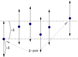
The tuple $x,y$ ($x<y\in D$) is a $\delta$-pair (or a pair of scale $\delta$) for $F$ if $|F(y)-F(x)|\geq\delta$ and for all $z\in D$, $x<z<y$ implies $|F(z)-F(x)|<\delta$ and $|F(y)-F(z)|<\delta$. A $\delta$-pair’s direction is increasing or decreasing according to whether $F(y)>F(x)$ or $F(y)<F(x)$.

$\delta$-Pairs having opposite directions cannot overlap but they may share an end point. $\delta$-Pairs of the same direction may overlap, but may not be nested. We use the term “$\ast$-pair” to indicate a $\delta$-pair having an unspecified $\delta$. We say that a $\ast$-pair is significant at scale $\delta$ if it is of scale $\delta^{\prime}$ for $\delta^{\prime}\geq\delta$. From a topological viewpoint, a $\ast$-pair is the pairing of critical points used to determine each extremum’s persistence [14].

Figure 1: A $\delta$-pair.

We define $\delta$-monotonicity as follows:

Definition 3.4.

Let $X$ be an interval, $F$ is $\delta$-monotonic on $X$ if all $\delta$-pairs in $X$ have the same direction; $F$ is strictly $\delta$-monotonic when there exists at least one such $\delta$-pair. In this case:

• $F$ is $\delta$-increasing on $X$ if $X$ contains an increasing $\delta$-pair.

• $F$ is $\delta$-decreasing on $X$ if $X$ contains a decreasing $\delta$-pair.

A $\delta$-monotonic interval $X$ satisfies $\textrm{OMAFE}(X)<\delta/2$. We say that a $\ast$-pair $x,y$ is maximal if whenever $z_{1},z_{2}$ is a $\ast$-pair of a larger scale in the same direction containing $x,y$, then there exists a $\ast$-pair $w_{1},w_{2}$ of an opposite direction contained in $z_{1},z_{2}$ and containing $x,y$. For example, the sequence $1,3,2,4$ has 2 maximal $\ast$-pairs: $1,4$ and $3,2$. Maximal $\ast$-pairs of opposite direction may share a common point, whereas maximal $\ast$-pairs of the same direction may not. Maximal $\ast$-pairs cannot overlap, meaning that it cannot be the case that exactly one end point of a maximal $\ast$-pair lies strictly between the end points of another maximal $\ast$-pair; either neither point lies strictly between or both do. In the case that both do, we say that the one maximal $\ast$-pair properly contains the other. All $\ast$-pairs must be contained in a maximal $\ast$-pair.

Lemma 3.5.

The smallest maximal $\ast$-pair containing a $\ast$-pair must be of the same direction.

Proof 3.6.

Suppose a $\ast$-pair is immediately contained in a maximal $\ast$-pair $W$. Suppose $W$ is not in the same direction, then within $W$, seek the largest $\ast$-pair in the same direction as $P$ and containing $P$, then it must be a maximal $\ast$-pair in $D$ since maximal $\ast$-pairs of different directions cannot overlap.

The first and second point of a maximal $\ast$-pair are extrema and the reverse is true as well as shown by the next lemma.

Lemma 3.7.

Every extremum is either the first or second point of a maximal $\ast$-pair.

Proof 3.8.

The case $x=x_{1}$ or $x=x_{n}$ follows by inspection. Otherwise, $x$ is the end point of a left and a right $\ast$-pair. Each $\ast$-pair must immediately belong to a maximal $\ast$-pair of same direction: a $\ast$-pair $P$ is contained in a maximal $\ast$-pair $M$ of same direction and there is no maximal $\ast$-pair $M^{\prime}$ of opposite direction such that $P\subset M^{\prime}\subset M$. Let $M^{l}$ and $M^{r}$ be the maximal $\ast$-pairs immediately containing the left and right $\ast$-pair of $x$. Suppose neither $M^{l}$ and $M^{r}$ have $x$ as a end point. Suppose $M^{l}\subset M^{r}$, then the right $\ast$-pair is not immediately contained in $M^{r}$, a contradiction. The result follows by symmetry.

Our approach is to label each extremum in $F$ with a scale parameter $\delta$ saying that this extremum is “significant” at scale $\delta$ and below. Our intuition is that by picking extrema at scale $\delta$, we should have a segmentation having error less than $\delta/2$.

Definition 3.9.

The scale labeling of an extremum $x$ is the maximum of the scales of the maximal $\ast$-pairs for which it is an end point.

For example, given the sequence $1,3,2,4$ with 2 maximal $\ast$-pairs ($1,4$ and $3,2$), we would give the following labels in order $3,1,1,3$.

Definition 3.10.

Given $\delta>0$, a maximal alternating sequence of $\delta$-extrema $Y=y_{1}\dots y_{K+1}$ is a sequence of extrema each having scale label at least $\delta$, having alternating types (maximum/minimum), and such that there exists no sequence properly containing $Y$ having these same properties. From $Y$ we define a maximal alternating $\delta$-segmentation of $D$ by segmenting at the points $x_{1},y_{2}\dots y_{K},x_{n}$.

Theorem 3.11.

Given $\delta>0$, let $P=S_{1}\dots S_{K}$ be a maximal alternating $\delta$-segmentation derived from maximal alternating sequence $y_{1}\dots y_{K+1}$ of $\delta$-extrema. Then any alternating segmentation $Q$ having OMAFE($Q$) $<$ OMAFE($P$) has at least $K+1$ segments.

Proof 3.12.

We show that conditions A and B of Proposition 3.1 are satisfied with $\epsilon=$ OMAFE($P$).

First we show that each segment $S_{i}$ is $\delta$-monotone; from this we conclude that $\textrm{OMAFE}(P)<\delta/2$. Intervals $[x_{1},y_{1}]$ and $[y_{K},x_{n}]$ contain no maximal $\ast$-pairs of scale $\delta$ or larger, and therefore contain no $\ast$-pairs of scale $\delta$ or larger. Similarly, no $[y_{i},y_{i+1}]$ contains an opposite-direction significant $\ast$-pair.

Condition A: Follows from $\delta$-monotonicity of each $S_{i}$ and maximal $\ast$-pairs not overlapping.

Condition B: We show that $|F(y_{i+1})-F(y_{i})|\geq\delta>2\times\textrm{OMAFE}(P)$. If $i=1$, then $y_{i}$ must begin an maximal $\ast$-pair, and the maximal $\ast$-pair must end with $y_{i+1}$ since maximal $\ast$-pairs cannot overlap. The case $i+1=k$ is similar. Otherwise, since maximal $\ast$-pairs cannot overlap, each $y_{i},y_{i+1}$ is either a maximal $\ast$-pair of scale $\delta$ or larger or there exist indices $j$ and $k$, $j<i$ and $k>i+1$ such that $y_{j},y_{i}$ is a maximal $\ast$-pair of scale at least $\delta$, and $y_{i+1},y_{k}$ is a maximal $\ast$-pair of scale at least $\delta$. These two maximal $\ast$-pairs have the same direction, and that this is opposite to the direction of $[y_{i}y_{i+1}]$. Now suppose $|F(y_{i})-F(y_{i+1})|<\delta$. Then $y_{j},y_{k}$ is a $\ast$-pair properly containing $y_{j}$, $y_{i}$ and $y_{i+1}$, $y_{k}$. But neither $y_{j},y_{i}$ nor $y_{i+1},y_{k}$ can be properly contained in a $\ast$-pair of opposite direction lying within $y_{j},y_{k}$, thus contradicting their maximality and proving the claim.

Sequences of extrema labeled at least $\delta$ are generally not maximal alternating. For example the sequence $0,10,9,10,0$ is scale labeled $10,10,1,10,10$. However, a simple relabeling of certain extrema can make them maximal alternating. Consider two same-sense extrema $z_{1}<z_{2}$ such that lying between them there exists no extremum having scale at least as large as the minimum of the two extrema’s scales. We must have $F(z_{1})=F(z_{2})$, since otherwise the point upon which $F$ has the lesser value could not be the endpoint of a maximal $\ast$-pair. This is the only situation which causes choice when constructing a maximal alternating sequence of $\delta$-extrema. To eliminate this choice, replace the scale label on $z_{1}$ with the largest scale of the opposite-sense extrema lying between them. In the next section, Algorithm 1 incorporates this re-labeling making Algorithm 2 simple and efficient.

3.1 Computing a Scale Labeling Efficiently

Algorithm 1 (next page) produces a scale labeling in linear time. Extrema from the original data are visited in order, and they alternate (maxima/minima) since we only pick one of the values when there are repeated values (such as $1,1,1$).

The algorithm has a main loop (lines 5 to 12) where it labels extrema as it identifies extremal $\ast$-pairs, and stack the extrema it cannot immediately label. At all times, the stack (line 3) contains minima and maxima in strictly increasing and decreasing order respectively. Also at all times, the last two extrema at the bottom of the stack are the absolute maximum and absolute minimum (found so far). Observe that we can only label an extrema as we find new extremal $\ast$-pairs (lines 7, 10, and 14).

• If the stack is empty or contains only one extremum, we simply add the new extremum (line 12).

• If there are only 2 extrema $z_{1},z_{2}$ in the stack and we found either a new absolute maximum or new absolute minimum ($z_{3}$), we can pop and label the oldest one ($z_{1}$) (lines 9, 10, and 11) because the old pair ($z_{1},z_{2}$) forms a maximal $\ast$-pair and thus must be bounded by extrema having at least the same scale while the oldest value ($z_{1}$) does not belong to a larger maximal $\ast$-pair. Otherwise, if there are only 2 extrema $z_{1},z_{2}$ in the stack and the new extrema $z_{3}$ satisfies $z_{3}\in(\min(z_{1},z_{2}),\max(z_{1},z_{2}))$, then we add it to the stack since no labeling is possible yet.

• While the stack contains more than 2 extrema (lines 6, 7 and 8), we consider the last three points on the stack ($s_{3},s_{2},s_{1}$) where $s_{1}$ is the last point added. Let $z$ be the value of the new extrema. If $z\in(\min(s_{1},s_{2}),\max(s_{1},s_{2}))$, then it is simply added to the stack since we cannot yet label any of these points; we exit the while loop. Otherwise, we have a new maximum (resp. minimum) exceeding (resp. lower) or matching the previous one on stack, and hence $s_{1},s_{2}$ is a maximal $\ast$-pair. If $z\neq s_{2}$, then $s_{3},z$ is a maximal $\ast$-pair and thus, $s_{2}$ cannot be the end of a maximal $\ast$-pair and $s_{1}$ cannot be the beginning of one, hence both $s_{2}$ and $s_{1}$ are labeled. If $z=s_{2}$ then we have successive maxima or minima and the same labeling as $z\neq s_{2}$ applies.

During the “unstacking” (lines 13 and following), we visit a sequence of minima and maxima forming increasingly larger maximal $\ast$-pairs.

The algorithm runs in time $O(n)$ (independent of $K$). Indeed, for any index of an extremum, the condition at line 6 will evaluate once to false; moreover the condition at line 6 cannot evaluate to true more than $O(n)$ times.

1:  INPUT: an array $d$ containing the $y$ values indexed from $0$ to $n-1$, repeated consecutive values have been removed

2:  OUTPUT: a scale labeling for all extrema

3:  $S\leftarrow$ empty stack, First($S$) is the value on top, Second($S$) is the second value

4:  define $\delta(d,S)=|d_{\textrm{First}(S)}-d_{\textrm{Second}(S)}|$

5:  for $e$ index of an extremum in $d$, $e$’s are visited in increasing order do

6:     while length($S$) $>2$ and ($e$ is a minimum such that $d_{e}\leq\textrm{Second}(S)$ or $e$ is a maximum such that $d_{e}\geq\textrm{Second}(S)$) do

7:        label First($S$) and Second($S$) with $\delta(d,S)$

8:        pop stack $S$ twice

9:     end while

10:     if length($S$) is 2 and ($e$ is a minimum such that $d_{e}\leq\textrm{Second}(S)$ or $e$ is a maximum such that $d_{e}\geq\textrm{Second}(S)$) then

11:        label Second($S$) with $\delta(d,S)$

12:        remove Second($S$) from stack $S$

13:     end if

14:     stack $e$ to $S$

15:  end for

16:  while length of $S$ $>2$ do

17:     label First($S$) with $\delta(d,S)$

18:     pop stack $S$

19:  end while

20:  label First($S$) and Second($S$) with $\delta(d,S)$

Algorithm 1 Algorithm to compute the scale labeling in $O(n)$ time.

Once the labeling is complete, we find $K+2$ extrema having largest scale in time $O(nK)$ using $O(K)$ memory, then we remove all extrema having the same scale as the smallest scale in these $K+2$ extrema (removing at least one), we replace the first and the last extrema by $0$ and $n-1$ respectively (see Algorithm 2). The result is an optimal segmentation having at most $K$ segments.

  INPUT: an array $d$ containing the $y$ values indexed from $1$ to $n$

  INPUT: $K$ a bound on the number of segments desired

  OUTPUT: unsorted segmentation points (a $\delta$-segmentation)

  $L\leftarrow$ empty array (capacity $K+3$)

  for $e$ is index of an extremum in $d$ having scale $\delta$, $e$ are visited in increasing order do

     insert $(e,\delta)$ in $L$ so that $L$ is sorted by scale in decreasing order (sort on $\delta$) using binary search

     if length of $L$ is $K+3$ then

        pop last(L)

     end if

  end for

  remove all elements of $L$ having the scale of last(L)

  RETURN: the indexes in $L$ replacing first one by $1$ and last one by $n$

Algorithm 2 Given the scale labeling, this algorithm will return a segmentation using at most $K$ segments. It is assumed that there are at least $K+1$ extrema to begin with.

Alternatively, if we plan to resegment the time series several times with different values of $K$, we can sort all extrema by their label in time $O(n\log n)$, and compute in time $O(n)$ an auxiliary structure on the sorted set so that when selecting the $i\textrm{th}$ item in the sorted list ($d_{i}$), we obtain the index $j$ of the earliest occurrence of this scale in the list ($\textrm{scale}(d_{j})=\textrm{scale}{d_{i}}$ and $\textrm{scale}(d_{j})<\textrm{scale}(d_{j-1})$ if $j>0$) in constant time. Hence, we can segment any time series optimally in constant time given this precomputation in time $O(n\log n)$.

Lemma 3.13.

Given a precomputation in time $O(n\log n)$ using $O(n)$ storage, for any desired upper bound on the number of segments $K$, we can compute the segmentation points of an optimal OMAFE, and the corresponding OMAFE value, in constant time.

Hence, we can compute an OMAFE versus $K$ plot in $O(n\log n)$ time.

  INPUT: Time Series $(x_{i},y_{i})$ of length $n$

  INPUT: Desired number of segments $K$

  INPUT: Function $E(p,q)$ computing linear fit error in range $[x_{p},x_{q}]$

  $S\leftarrow(1,n,E(0,n))$

  while  $|S|<K$  do

     find tuple $(i,j,\epsilon)$ in $S$ with maximum last entry

     find minimum of $E(i,l)+E(l+1,j)$ for $l=i,\ldots,j-1$

     remove tuple $(i,j,\epsilon)$ from $S$

     insert tuples $(i,l,E(i,l))$ and $(l,j,E(l+1,j))$ in $S$

  end while

  $S$ contains the segmentation

Algorithm 3 Piecewise Linear Top-Down Segmentation Heuristic.

  INPUT: Time Series $(x_{i},y_{i})$ of length $n$

  INPUT: Desired number of segments $K$

  INPUT: Function $E(p,q)$ computing linear fit error in range $[x_{p},x_{q}]$

  $S\leftarrow[0,0],[1,1],[2,2],\ldots,[n,n]$

  while  $|S|>K$  do

     find consecutive intervals in $S$, $[p_{1},p_{2}]$ and $[p_{2}+1,p_{3}]$, having minimal value $E(p_{1},p3)-E(p_{1},p_{2})-E(p_{2}+1,p_{3})$

     merge the two consecutive intervals

  end while

  $S$ contains the segmentation

Algorithm 4 Piecewise Linear Bottom-Up Segmentation Heuristic.

4 Experimental Results and Comparison to Piecewise Linear Segmentation Heuristics

We compare our optimal $O(nK)$ algorithm with our implementations of two piecewise linear segmentation heuristics [3]: top-down, which runs in $O(nK)$ time (see Algorithm 3), and bottom-up which runs in $O(n(n-K))$ time (see Algorithm 4). The top-down heuristic successively segments the data starting with only one segment, each time picking the segment with the worse linear regression error and finding the best segmentation point; the linear regression is not continuous from one segment to the other. The regression error can be computed in constant time if one has precomputed the range moments [15, 16]. The bottom-up heuristic starts with intervals containing only one data point and successively merge them, each time choosing the least expensive merge. By maintaining the segments in a doubly-linked list coupled with a heap or tree, it is possible to obtain a bottom-up heuristic with $O((n-K)\log n)$ complexity, but it then uses much more memory and it is more difficult to implement.

Once the piecewise linear segmentation is completed, we run through the segments and aggregate consecutive segments having the same sign where the sign of a segment $[y_{k},y_{k+1}]$ is defined by $F(y_{k+1})-F(y_{k})$, setting 0 to be a positive sign (increasing monotonicity).

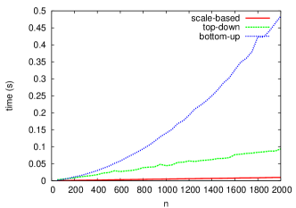
We implemented all algorithms in Python (version 2.5) and ran the experiments on a 2.16 GHz Intel Core 2 Duo processor with sufficient RAM (1 GB). Fig. 2 presents the relative speed of the various segmentation algorithms on time series of various lengths for a fixed number of segments (using randomly generated data). The timings reported include all pre-processing.

Figure 2: Time to segment a time series of length $n$ in $K=20$ segments.

4.1 Electrocardiograms (ECG)

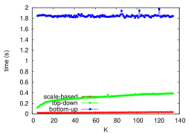
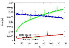
ECGs have a well known monotonicity structure with 5 commonly identifiable extrema per pulse (reference points P, Q, R, S, and T) (see Fig. 3) though not all points can be easily identified on all pulses and the exact morphology can vary. We used freely available samples from the MIT-BIH Arrhythmia Database [17]. We only present our results over one sample (labeled “100.dat”) since we found that results did not vary much between data samples. These ECG recordings used a sampling rate of 360 Hz per channel with 11-bit resolution (see Fig. 4(a)). We keep the first 4000 samples (11 seconds) and about 14 pulses, and we do no preprocessing such as baseline correction. We can estimate that a typical pulse has about 5 “easily” identifiable monotonic segments. Hence, out of 14 pulses, we can estimate that there are about 70 significant monotonic segments, some of which match the domain-specific markers (reference points P, Q, R, S, and T). A qualitative description of such data is useful for pattern matching applications.

Figure 3: Schema of an ECG pulse with commonly identified reference points (PQRST).

The running time as a function of $K$ is presented in Fig. 4(b). The scale-based segmentation implementation is faster than our implementations of the piecewise linear heuristics. On such a long time series (4000 samples), our implementation of the bottom-up heuristic is much slower than the alternatives.

(a) Time Series

(b) Time vs. number of segments $K$

(c) OMAFE vs. number of segments $K$

Figure 4: Results of experiments over ECG data.

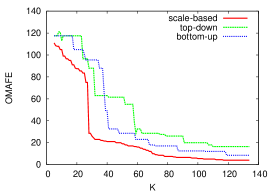
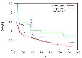
We want to determine how well the piecewise linear segmentation heuristics do comparatively. OMAFE is an absolute and not relative error measure, but because the range of the ECGs under consideration is roughly between 950 and 1150, we expect the OMAFE to never exceed 100 by much. The OMAFE with respect to the maximal number of segments ($K$) is given in Fig. 4(c): it is a “monotonicity spectrum.” By counting on about 5 monotonic segments per pulse with a total of 14 pulses, there should about 70 monotonic segments in the 4000 samples under consideration. We see that the decrease in OMAFE with the addition of new segments starts to level off between 50 and 70 segments as predicted. The addition of new segments past 70 ($K>70$) has little impact. The scale-based algorithm is optimal, but also at least 3 times more accurate than the top-down algorithm for larger $K$ and this is consistent over other data sets. In fact, the OMAFE becomes practically zero for $K>80$ whereas the OMAFE of the top-down linear regression algorithm remains at around 20, which is still significant. The bottom-up heuristic is more accurate than the top-down heuristic, but it still has about twice the OMAFE for large $K$. OMAFE of the scale-based algorithm is a non increasing function of $K$, a consequence of optimality.

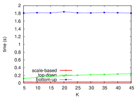
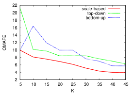
4.2 Temperature Recordings

We consider the daily temperature recordings of the first of 35 weather stations in the MD*Base Daily temperature data set [18]. Since we only have one year of recordings, only 365 data points are used (see Fig. 5(a)). We also give the running times (see Fig. 5(b)) and the accuracy (see Fig. 5(c)). Our implementation of the bottom-up heuristic is now much faster due to small size of the times series, but the OMAFE, while superior to the top-down heuristic, exhibits a spurious spike near $K=40$, showing the danger of relying on a piecewise linear heuristic to study the monotonicity of a data set. Considering the OMAFE of our scale-based algorithm, we notice that the accuracy increases slowly after $K=10$.

(a) Time Series

(b) Time vs. number of segments $K$

(c) OMAFE vs. number of segments $K$

Figure 5: Results of experiments over daily temperature data.

4.3 Synthetic Random Walk Data

Random walks are often used as models for common time series such as stock prices. We generated a random walk $(i,y_{i})_{i=1,\ldots,4000}$ using the formula $y_{i+1}=y_{i}+\epsilon$ where $\epsilon\sim N(0,1)$ (see Fig. 6(a)). The running times are nearly identical to the ECG case, as is expected since the time series have the same length. However, the OMAFE differs (see Fig. 6(c)): using our optimal algorithm, the curve is smooth with no sharp drop. Meanwhile, the bottom-up heuristic exhibits another spurious spike in the OMAFE (around $K=20$) while it provides the optimal segmentation at $K=5$.

(a) Time Series

(b) Time vs. number of segments $K$

(c) OMAFE vs. number of segments $K$

Figure 6: Results of experiments over random walk.

5 Conclusion and Future Work

We presented optimal and fast algorithms to compute the best piecewise monotonic segmentation in time $O(n)$ and the complete OMAFE-versus-$K$ spectrum in time $O(n\log n)$. Our experimental results suggest that one should be careful when deriving monotonicity information from piecewise linear segmentation heuristics. Future work will focus on choosing the optimal number of segments for given applications. We also plan to investigate the applications of the monotonicity spectrum as a robust analysis. Further work to integrate flat segments is needed [5, 16].

References

- [1] D. Lemire, M. Brooks, and Y. Yan, “An optimal linear time algorithm for quasi-monotonic segmentation,” in ICDM 2005, 2005.
- [2] E. Bingham, A. Gionis, N. Haiminen, H. Hiisilä, H. Mannila, and E. Terzi, “Segmentation and dimensionality reduction,” in SDM 2006, 2006.
- [3] E. J. Keogh, S. Chu, D. Hart, and M. J. Pazzani, “An online algorithm for segmenting time series,” in ICDM 2001, pp. 289–296, 2001.
- [4] N. Haiminen and A. Gionis, “Unimodal segmentation of sequences,” in ICDM 2004, 2004.
- [5] M. Brooks, Y. Yan, and D. Lemire, “Scale-based monotonicity analysis in qualitative modelling with flat segments,” in IJCAI 2005, 2005.
- [6] W. Fitzgerald, D. Lemire, and M. Brooks, “Quasi-monotonic segmentation of state variable behavior for reactive control,” in AAAI 2005, 2005.
- [7] D. G. Galati and M. A. Simaan, “Automatic decomposition of time series into step, ramp, and impulse primitives,” Pattern Recognition, vol. 39, pp. 2166–2174, November 2006.
- [8] J. Han, W. Gong, and Y. Yin, “Mining segment-wise periodic patterns in time-related databases,” in KDD 1998, 1998.
- [9] E. J. Keogh and M. J. Pazzani, “An enhanced representation of time series which allows fast and accurate classification, clustering and relevance feedback,” in KDD 1998, pp. 239–243, 1998.
- [10] D. Šuc and I. Bratko, “Induction of qualitative tree,” in ECML 2001, pp. 442–453, Springer, 2001.
- [11] V. A. Ubhaya, S. E. Weinstein, and Y. Xu, “Best piecewise monotone uniform approximation,” Approx. Theory, vol. 63, pp. 375–383, December 1990.
- [12] V. A. Ubhaya, “Isotone optimization I,” Approx. Theory, vol. 12, pp. 146–159, 1974.
- [13] M. Brooks, “Approximation complexity for piecewise monotone functions and real data,” Computers and Mathematics with Applications, vol. 27, no. 8, 1994.
- [14] H. Edelsbrunner, D. Letscher, and A. Zomorodian, “Topological persistence and simplification,” Discrete Comp. Geo., vol. 28, pp. 511–533, 2002.
- [15] D. Lemire, “Wavelet-based relative prefix sum methods for range sum queries in data cubes,” in CASCON 2002, IBM, 2002.
- [16] D. Lemire, “A better alternative to piecewise linear time series segmentation,” in SDM 2007, 2007.
- [17] A. L. Goldberger et al., “PhysioBank, PhysioToolkit, and PhysioNet,” Circulation, vol. 101, no. 23, pp. 215–220, 2000. http://www.physionet.org/physiobank/database/mitdb/ – last checked in April 2007.
- [18] Institute for Statistics and Econometrics, “MD*Base Online,” 2007. http://www.quantlet.org/mdbase/ – last checked in April 2007.
- [19] J. O. Ramsay and B. W. Silverman, The Analysis of Functional Data. Springer, 1997.