Parameter estimation in diagonalizable bilinear
stochastic parabolic equations

Abstract

A parameter estimation problem is considered for a stochastic parabolic equation with multiplicative noise under the assumption that the equation can be reduced to an infinite system of uncoupled diffusion processes. From the point of view of classical statistics, this problem turns out to be singular not only for the original infinite-dimensional system but also for most finite-dimensional projections. This singularity can be exploited to improve the rate of convergence of traditional estimators as well as to construct completely new closed-form exact estimator.

Primary 62F12; Secondary 60H15

1 Introduction

In the classical statistical estimation problem, the starting point is a family $\mathbf{P}^{\theta}$ of probability measures depending on the parameter $\theta$ belonging to some subset $\Theta$ of a finite-dimensional Euclidean space. Each $\mathbf{P}^{\theta}$ is the distribution of a random element. It is assumed that a realization of one random element corresponding to one value $\theta=\theta_{0}$ of the parameter is observed, and the objective is to estimate the values of this parameter from the observations.

The intuition is to select the value $\theta$ corresponding to the random element that is most likely to produce the observations. A rigorous mathematical implementation of this idea leads to the notion of the regular statistical model [10]: the statistical model (or estimation problem) $\mathbf{P}^{\theta},\ \theta\in\Theta$, is called regular, if the following two conditions are satisfied:

• there exists a probability measure $\mathbf{Q}$ such that all measures $\mathbf{P}^{\theta}$ are absolutely continuous with respect to $\mathbf{Q}$;

• the density $d\mathbf{P}^{\theta}/d\mathbf{Q}$, called the likelihood ratio, has a special property, called local asymptotic normality.

If at least one of the above conditions is violated, the problem is called singular.

In regular models, the estimator $\widehat{\theta}$ of the unknown parameter is constructed by maximizing the likelihood ratio and is called the maximum likelihood estimator (MLE). Since, as a rule, $\widehat{\theta}\not=\theta_{0}$, the consistency of the estimator is studied, that is, the convergence of $\widehat{\theta}$ to $\theta_{0}$ as more and more information becomes available. In all known regular statistical problems, the amount of information can be increased in one of two ways: (a) Increasing the sample size, for example, the observation time interval (large sample asymptotic); (b) reducing the amplitude of noise (small noise asymptotic). The asymptotic behavior of $\widehat{\theta}$ in both cases is well-studied. It is also known that many other estimators in regular models are asymptotically equivalent to the MLE.

While all regular models are in a sense the same, each singular model is different. Sometimes, it is possible to approximate a singular model with a sequence of regular models. For each regular model, an MLE is constructed, and then in the limit one can often get the true value of the parameter while both the sample size and the noise amplitude are fixed. Some singular models cannot be approximated by a sequence of regular models and admit estimators that have nothing to do with the MLE [14]. In this paper, Section 4, we introduce a completely new type of such estimators for a large class of singular models.

Infinite-dimensional stochastic evolution equations, that is, stochastic evolution equations in infinite-dimensional spaces, are a rich source of statistical problems, both regular and singular. A typical example is the Itô equation

$$\begin{cases}du(t)+(\mathcal{A}_{0}+\theta\mathcal{A}_{1})u(t)dt=f(t)dt+\sum\limits_{j\geq 1}(\mathcal{M}_{j}u(t)+g_{j}(t))dW_{j}(t),\\ u(0)=u_{0},\end{cases}$$ (1.1)

where $t\in[0,T],\ \mathcal{A}_{0},\ \mathcal{A}_{1},\ \mathcal{M}_{j}$ are linear operators, $f,\ g_{j}$ are adapted processes, $W_{j}$ are independent Wiener processes, and $\theta$ is the unknown parameter belonging to an open subset of the real line. The underlying assumption is that the solution $u$ exists, is unique, and can be observed as an infinite-dimensional object for all $t\in[0,T]$. Depending on the operators in the equation, the estimation model can be regular, a singular limit of regular problems, or completely singular.

If $\mathcal{A}_{0},\mathcal{A}_{1},\ \mathcal{M}_{j}$ are partial differential or pseudo-differential operators, (1.1) becomes a stochastic partial differential equation (SPDE), which is becoming increasingly popular for modelling various phenomena in fluid mechanics [25], oceanography [21], temperature anomalies [4, 22], finance [3, 5, 6], and other domains. Various estimation problems for different types of SPDEs have been investigated by many authors: [1, 2, 7, 8, 9, 11, 12, 13, 17, 18, 19, etc.].

Depending on the stochastic part, (1.1) is classified as follows:

• equation with additive noise, if $\mathcal{M}_{j}=0$ for all $j$;

• equation with multiplicative noise (or bilinear equation) otherwise.

Depending on the operators, (1.1) is classified as follows:

• Diagonalizable equation, if the operators $\mathcal{A}_{0}$, $\mathcal{A}_{1}$, and $\mathcal{M}_{j}$, $j\geq 1$, have a common system of eigenfunctions $h_{k},\ k\geq 1$, and this system is an orthonormal basis in a suitable Hilbert space.

• Non-diagonalizable equation otherwise.

A diagonalizable equation is reduced to an infinite system of uncoupled one-dimensional diffusion processes; these processes are the Fourier coefficients of the solution in the basis $h_{k}$. As a result, while somewhat restrictive as a modelling tool, diagonalizable equations are an extremely convenient object to study estimation problems and often provide the benchmark results that carry over to more general equations.

The parameter estimation problem for a diagonalizable equation (1.1) with additive space-time white noise (that is, $g_{j}=h_{j}$ and $\mathcal{M}_{j}=0$ for all $j$) was studied for the first time by Huebner, Khasminskii, and Rozovskii [8], and further investigated in [7, 8, 9, 23]. The main feature of this problem is that every $N$-dimensional projection of the equation leads to a regular statistical problem, but the problem can become singular in the limit $N\to\infty$ (a singular limit of regular problems); when this happens, the dimension $N$ of the projection becomes a natural asymptotic parameter of the problem. Once the diagonalizable model is well-understood, extensions to more general equations can be considered ([18, 19]).

This paper is the first attempt to investigate the estimation problem for infinite-dimensional bilinear equations. Such models are often completely singular, that is, cannot be represented as a limit of regular models. We consider the more tractable situation of diagonalizable equations. In Section 2 we provide the necessary background on stochastic evolution equations, with emphasis on diagonalizable bilinear equations. The maximum likelihood estimator (MLE) and its modifications for diagonalizable bilinear equations are studied in Section 3. We give sufficient conditions on operators $\mathcal{A}_{0},\mathcal{A}_{1},\mathcal{M}$ that ensure consistency and asymptotic normality of the MLE. We also demonstrate that the MLE in this model is not always the best estimator, which, for a singular model is not at all surprising. Section 4 emphasizes the point even more by introducing a closed-form exact estimator. Due to the specific structure of stochastic term, for a large class of infinite-dimensional systems with finite-dimensional noise, one can get the exact value of the unknown parameter after a finite number of arithmetic manipulations with the observations. The very existence of such estimators in these models is rather remarkable and has no analogue in classical statistics.

As an illustration, let $\theta$ be a positive number, $W$ a standard Wiener process, and consider the Itô equation

$$du(t,x)-\theta u_{xx}(t,x)dt=u(t,x)dW(t),\ t>0,\ x\in(0,\pi),$$ (1.2)

with zero boundary conditions. If $h_{k}(x)=\sqrt{2/\pi}\,\sin(kx)$, $k\geq 1,$ and

$$u_{k}(t)=\int_{0}^{\pi}u(t,x)h_{k}(x)dx\ ,$$

then

$$u(t,x)=\sum_{k\geq 1}u_{k}(t)h_{k}(x)$$ (1.3)

and each $u_{k}$ is a geometric Brownian motion:

$$u_{k}(t)=u_{k}(0)-\int_{0}^{t}k^{2}u_{k}(s)ds+\int_{0}^{t}u_{k}(s)dW(s).$$

We assume that $u_{k}(0)\not=0$ for all $k\geq 1$. In Sections 3 and 4 we establish the following result.

Theorem 1.1.

If the solution of equation (1.2) is observed in the form (1.3), then the parameter $\theta$ can be computed in each of the following ways:

1. $\displaystyle\theta=\lim_{T\to\infty}\left(\frac{1}{k^{2}T}\ln\frac{u_{k}(0)}{u_{k}(T)}-\frac{1}{2k^{2}}\right)$ for every $k\geq 1$;

2. $\displaystyle\theta=\lim_{k\to\infty}\frac{1}{k^{2}T}\ln\frac{u_{k}(0)}{u_{k}(T)}$ for every $T>0$;

3. $\displaystyle\theta=\frac{1}{T(k^{2}-n^{2})}\ln\frac{u_{n}(T)u_{k}(0)}{u_{k}(T)u_{n}(0)}$ for every $T>0$ and $n\not=k$.

Both (E1) and (E2) are essentially the same maximum likelihood estimator, but the infinite-dimensional nature of the equation makes it possible to study this estimator in two different asymptotic regimes. (E3) is a closed-form exact estimator. While it is most likely to be the best choice for this particular problem, we show in Section 4 that computational complexity of closed-form exact estimators can dramatically increase with the number of Wiener processes driving the equation, while the complexity of the MLE is almost unaffected by this number. The result is another unexpected feature of closed-form exact estimators: ever though they produce the exact value of the parameter, they are not always the best choice computationally.

2 Stochastic Parabolic Equations

In this section we introduce the diagonalizable stochastic parabolic equation depending on a parameter and study the main properties of the solution.

Let $\mathbf{H}$ be a separable Hilbert space with the inner product $(\cdot,\cdot)_{0}$ and the corresponding norm $\|\cdot\|_{0}$. Let $\Lambda$ be a densely-defined linear operator on $\mathbf{H}$ with the following property: there exists a positive number $c$ such that $\|\Lambda u\|_{0}\geq c\|u\|_{0}$ for every $u$ from the domain of $\Lambda$. Then the operator powers $\Lambda^{\gamma},\ \gamma\in\mathbb{R},$ are well defined and generate the spaces $\mathbf{H}^{\gamma}$: for $\gamma>0$, $\mathbf{H}^{\gamma}$ is the domain of $\Lambda^{\gamma}$; $\mathbf{H}^{0}=\mathbf{H}$; for $\gamma<0$, $\mathbf{H}^{\gamma}$ is the completion of $\mathbf{H}$ with respect to the norm $\|\cdot\|_{\gamma}:=\|\Lambda\cdot\|_{0}$ (see for instance Krein at al. [15]). By construction, the collection of spaces $\{\mathbf{H}^{\gamma},\ \gamma\in\mathbb{R}\}$ has the following properties:

• $\Lambda^{\gamma}(\mathbf{H}^{r})=\mathbf{H}^{r-\gamma}$ for every $\gamma,r\in\mathbb{R}$;

• For $\gamma_{1}<\gamma_{2}$ the space $\mathbf{H}^{\gamma_{2}}$ is densely and continuously embedded into $\mathbf{H}^{\gamma_{1}}$: $\mathbf{H}^{\gamma_{2}}\subset\mathbf{H}^{\gamma_{1}}$ and there exists a positive number $c_{12}$ such that $\|u\|_{\gamma_{1}}\leq c_{12}\|u\|_{\gamma_{2}}$ for all $u\in\mathbf{H}^{\gamma_{2}}$ ;

• for every $\gamma\in\mathbb{R}$ and $m>0$, the space $\mathbf{H}^{\gamma-m}$ is the dual of $\mathbf{H}^{\gamma+m}$ relative to the inner product in $\mathbf{H}^{\gamma}$, with duality $\langle\cdot,\cdot\rangle_{\gamma,m}$ given by

  $$\langle u_{1},u_{2}\rangle_{\gamma,m}=(\Lambda^{\gamma-m}u_{1},\Lambda^{\gamma+m}u_{2})_{0},\ {\rm where\ }u_{1}\in\mathbf{H}^{\gamma-m},\ u_{2}\in\mathbf{H}^{\gamma+m}.$$

Let $(\Omega,\mathcal{F},\{\mathcal{F}_{t}\},\mathbb{P})$ be a stochastic basis with the usual assumptions, and let $\{W_{j},\ j\geq 1\}$ be a collection of independent standard Brownian motions on this basis. Consider the following Itô equation

$$\begin{cases}du(t)+(\mathcal{A}_{0}+\theta\mathcal{A}_{1})u(t)dt=f(t)dt+\sum\limits_{j\geq 1}(\mathcal{M}_{j}u(t)+g_{k}(t))dW_{j}(t),\ 0<t\leq T,\\ u(0)=u_{0}\,\end{cases}$$ (2.1)

where $\mathcal{A}_{0},\,\mathcal{A}_{1},\,\mathcal{M}_{j}$ are linear operators, $f$ and $g_{k}$ are adapted process, and $\theta$ is a scalar parameter belonging to an open set $\Theta\subset\mathbb{R}$.

Definition 2.1.

(a) Equation (2.1) is called an equation with additive noise if $\mathcal{M}_{j}=0$ for all $j\geq 1$. Otherwise, (2.1) is called an equation with multiplicative noise (also known as a bilinear equation).
(b) Equation (2.1) is called diagonalizable if the operators $\mathcal{A}_{0},\ \mathcal{A}_{1},\mathcal{M}_{j},\ j\geq 1$, have a common system of eigenfunctions $\{h_{k},\ k\geq 1\}$ such that $\{h_{k},\ k\geq 1\}$ is an orthonormal basis in $\mathbf{H}$ and each $h_{k}$ belongs to every $\mathbf{H}^{\gamma}$.
(c) Equation (2.1) is called parabolic in the triple $(\mathbf{H}^{\gamma+m},\mathbf{H}^{\gamma},\mathbf{H}^{\gamma-m})$ if

• the operator $\mathcal{A}_{0}+\theta\mathcal{A}_{1}$ is uniformly bounded from $\mathbf{H}^{\gamma+m}$ to $\mathbf{H}^{\gamma-m}$ for $\theta\in\Theta:$ there exists a positive real number $C_{1}$ such that

  $$\|(\mathcal{A}_{0}+\theta\mathcal{A}_{1})v\|_{\gamma-m}\leq C_{1}\|v\|_{\gamma+m}$$ (2.2)

  for all $\theta\in\Theta$, $v\in\mathbf{H}^{\gamma+m}$;

• There exists a positive number $\delta$ and a real number $C$ such that, for every $v\in\mathbf{H}^{\gamma+m}$, $\theta\in\Theta$,

  $$-2\langle(\mathcal{A}_{0}+\theta\mathcal{A}_{1})v,v\rangle_{\gamma,m}+\sum_{j\geq 1}\|\mathcal{M}_{j}v\|_{\gamma}^{2}+\delta\|v\|_{\gamma+m}^{2}\leq C\|v\|_{\gamma}^{2}.$$ (2.3)

Remark 2.2.

(a) Note that (2.2) and (2.3) imply uniform continuity of the family of operators $\mathcal{M}_{j}$, $j\geq 1$ from $\mathbf{H}^{\gamma+m}$ to $\mathbf{H}^{\gamma}$; in fact,

$$\sum_{j\geq 1}\|\mathcal{M}_{j}v\|_{\gamma}^{2}\leq 2C_{1}\|v\|_{\gamma+m}^{2}+C\|v\|_{\gamma}^{2}.$$

(b) If equation (2.1) is parabolic, then condition (2.3) implies that

$$\langle(2\mathcal{A}_{0}+2\theta\mathcal{A}_{1}+CI)v,v\rangle_{\gamma,m}\geq\delta\|v\|_{\gamma+m}^{2},$$

where $I$ is the identity operator. The Cauchy-Schwartz inequality and the continuous embedding of $\mathbf{H}^{\gamma+m}$ into $\mathbf{H}^{\gamma}$ then imply

$$\|(2\mathcal{A}_{0}+2\theta\mathcal{A}_{1}+CI)v\|_{\gamma}\geq\delta_{1}\|v\|_{\gamma}$$

for some $\delta_{1}>0$ uniformly in $\theta\in\Theta$. As a result, we can take $\Lambda=(2\mathcal{A}_{0}+2\theta^{*}\mathcal{A}_{1}+CI)^{1/(2m)}$ for some fixed $\theta^{*}\in\Theta$.

From now on, if equation (2.1) is parabolic and diagonalizable, we will assume that the operator $\Lambda$ has the same eigenfunctions as the operators $\mathcal{A}_{0},\ \mathcal{A}_{1},\ \mathcal{M}_{j}$; by Remark 2.2, this leads to no loss of generality.

Example 1.

(a) For $0<t\leq T$ and $x\in(0,1)$, consider the equation

$$du(t,x)-\theta\,u_{xx}(t,x)dt=u_{x}(t,x)dW(t)$$ (2.4)

with periodic boundary conditions; $u_{x}=\partial u/\partial x$. Then $\mathbf{H}^{\gamma}$ is the Sobolev space on the unit circle (see, for example, Shubin [26, Section I.7]) and $\Lambda=\sqrt{I-\boldsymbol{\Delta}}$, where $\boldsymbol{\Delta}$ is the Laplace operator on $(0,1)$ with periodic boundary conditions. Direct computations show that equation (2.4) is diagonalizable; it is parabolic if and only if $2\theta>1$.

(b) Let $G$ be a smooth bounded domain in $\mathbb{R}^{d}$. Let $\boldsymbol{\Delta}$ be the Laplace operator on $G$ with zero boundary conditions. It is known (for example, from Shubin [26]), that

1. the eigenfunctions $\{h_{k},\ k\geq 1\}$ of $\boldsymbol{\Delta}$ are smooth in $G$ and form an orthonormal basis in $L_{2}(G)$;

2. the corresponding eigenvalues $\sigma_{k},\ k\geq 1$, can be arranged so that $0<-\sigma_{1}\leq-\sigma_{2}\leq\ldots$, and there exists a number $c>0$ such that $|\sigma_{k}|\sim ck^{2/d}$, that is,

   $$\lim_{k\to\infty}|\sigma_{k}|k^{-2/d}=c.$$

We take $\mathbf{H}=L_{2}(G)$, $\Lambda=\sqrt{I-\boldsymbol{\Delta}}$, where $I$ is the identity operator. Then $\|\Lambda u\|_{0}\geq\sqrt{1-\sigma_{1}}\|u\|_{0}$ and the operator $\Lambda$ generates the Hilbert spaces $\mathbf{H}^{\gamma}$, and, for every $\gamma\in\mathbb{R}$, the space $\mathbf{H}^{\gamma}$ is the closure of the set of smooth compactly supported function on $G$ with respect to the norm

$$\left(\sum_{k\geq 1}(1+k^{2})^{\gamma}|\varphi_{k}|^{2}\right)^{1/2},\ {\rm\ where\ }\varphi_{k}=\int_{G}\varphi(x)h_{k}(x)dx,$$

which is an equivalent norm in $\mathbf{H}^{\gamma}$. Let $\theta$ and $\sigma$ be real numbers. Then the stochastic equation

$$du-\theta\boldsymbol{\Delta}udt=\Lambda u\,dW$$ (2.5)

is

• always diagonalizable;

• parabolic in $(\mathbf{H}^{\gamma+1},\mathbf{H}^{\gamma},\mathbf{H}^{\gamma-1})$ for every $\gamma\in\mathbb{R}$ if and only if $2\theta>1$.

Indeed, we have $\mathcal{A}_{0}=0$, $\mathcal{A}_{1}=-\boldsymbol{\Delta}$, $\mathcal{M}_{1}=\Lambda$, $\mathcal{M}_{j}=0$, $j\geq 2$, and

$$-2\theta\langle\mathcal{A}_{1}v,v\rangle_{\gamma,1}=-2\theta\|v\|_{\gamma+1}^{2}+2\theta\|u\|_{\gamma}^{2},$$

and so (2.3) holds with $\delta=2\theta-1$ and $C=2\theta$.

Remark 2.3.

Taking in (2.1) $\mathbf{H}=L_{2}(G)$, where $G$ is a smooth bounded domain in $\mathbb{R}^{d}$, and $\mathcal{A}_{0}=-\boldsymbol{\Delta}$, $\mathcal{A}_{1}=I$, $\mathcal{M}_{j}u=h_{k}(x)u(x)$, $g_{k}=h_{k}(x)g(t,x)$, we get a bilinear equation driven by space-time white noise. Direct analysis shows that this equation is not diagonalizable. Moreover, the equation is parabolic if and only if $d=1$, that is, when $G$ is an interval; for details, see the lecture notes by Walsh [27].

For a diagonalizable equation, the parabolicity condition (2.3) can be expressed in terms of the eigenvalues of the operators in the equation.

Theorem 2.4.

Assume that equation (2.1) is diagonalizable, and

$$\mathcal{A}_{0}h_{k}=\rho_{k}h_{k},\ \mathcal{A}_{1}h_{k}=\nu_{k}h_{k},\ \mathcal{M}_{j}h_{k}=\mu_{jk}h_{k}.$$

With no loss of generality (see Remark 2.2), we also assume that

$$\Lambda h_{k}=\lambda_{k}h_{k}.$$

Then equation (2.1) is parabolic in the triple $(\mathbf{H}^{\gamma+m},\mathbf{H}^{\gamma},\mathbf{H}^{\gamma-m})$ if and only if there exist positive real numbers $\delta,C_{1}$ and a real number $C_{2}$ such that, for all $k\geq 1$ and $\theta\in\Theta$,

$$\lambda_{k}^{-2m}|\rho_{k}+\theta\nu_{k}|\leq C_{1};$$ (2.6)

$$-2(\rho_{k}+\theta\nu_{k})+\sum_{j\geq 1}|\mu_{jk}|^{2}+\delta\lambda_{k}^{2m}\leq C_{2}.$$ (2.7)

Proof.

We show that, for a diagonalizable equation, (2.6) is equivalent to (2.2) and (2.7) is equivalent to (2.3). Indeed, note that for every $\gamma,\ r\in\mathbb{R}$,

$$\|h_{k}\|_{\gamma+r}=\|\Lambda^{r}h_{k}\|_{\gamma}=\lambda_{k}^{r}\|h_{k}\|_{\gamma}.$$

Then (2.6) is (2.2) with $v=h_{k}$, and (2.7) is (2.3) with $v=h_{k}$. Since both (2.6) and (2.7) are uniform in $k$ and the collection $\{h_{k},\ k\geq 1\}$ is dense in every $\mathbf{H}^{\gamma}$, the proof of the theorem is complete. ∎

The following is the basic existence/uniqueness/regularity result for parabolic equations; for the proof, see Rozovskii [24, Theorem 3.2.1].

Theorem 2.5.

Assume that equation (2.1) is parabolic in the triple $(\mathbf{H}^{\gamma+m},\mathbf{H}^{\gamma},\mathbf{H}^{\gamma-m})$ and

1. the initial condition $u_{0}$ is deterministic and belongs to $\mathbf{H}^{\gamma}$;

2. the process $f=f(t)$ is $\mathcal{F}_{t}$-adapted with values in $\mathbf{H}^{\gamma-m}$ and

   $$\mathbb{E}\int_{0}^{T}\|f(t)\|_{\gamma-m}^{2}dt<\infty;$$

3. each process $g_{k}=g_{k}(t)$ is $\mathcal{F}_{t}$-adapted with values in $\mathbf{H}^{\gamma}$ and

   $$\sum_{j\geq 1}\mathbb{E}\int_{0}^{T}\|g_{j}(t)\|_{\gamma}^{2}<\infty.$$

Then there exists a unique $\mathcal{F}_{t}$-adapted process $u=u(t)$ with the following properties:

• $u\in L_{2}(\Omega;L_{2}((0,T);\mathbf{H}^{\gamma+m})\bigcap L_{2}(\Omega;C((0,T);\mathbf{H}^{\gamma}))$;

• $u$ is a solution of (2.1), that is, the equality

  $$\begin{split}u(t)+\int_{0}^{t}(\mathcal{A}_{0}+\theta\mathcal{A}_{1})u(s)ds&=u_{0}+\int_{0}^{t}f(s)ds\\ &+\sum_{j\geq 1}(\mathcal{M}_{j}u(s)+g_{k}(s))dW_{j}(s).\end{split}$$

  holds in $\mathbf{H}^{\gamma-m}$ for all $t\in[0,T]$ on the same set $\Omega^{\prime}\subset\Omega$ of probability one;

• There exists a positive real number $C_{0}$ depending only on $T$ and the numbers $C,\delta$ in (2.3) such that

  $$\begin{split}\mathbb{E}\sup_{0<t<T}\|u(t)\|_{\gamma}^{2}+\mathbb{E}\int_{0}^{T}\|u(t)\|_{\gamma+m}^{2}dt&\leq C_{0}\left(\|u_{0}\|_{\gamma}^{2}+\mathbb{E}\int_{0}^{T}\|f(t)\|_{\gamma-m}^{2}dt\right.\\ &+\left.\sum_{j\geq 1}\mathbb{E}\int_{0}^{T}\|g_{j}(t)\|_{\gamma}^{2}\right)\end{split}$$

Corollary 2.6.

Assume that equation (2.1) is parabolic and diagonalizable. Then, under the assumptions of Theorem 2.5 we have

$$u(t)=\sum_{k=1}^{\infty}u_{k}(t)h_{k}{\rm\ and}\sum_{k=1}^{\infty}\lambda_{k}^{2\gamma}\mathbb{E}|u_{k}(t)|^{2}<\infty,\ t\in[0,T],$$ (2.8)

where $u_{k}(t)=(\Lambda^{\gamma}u(t),h_{k})_{0}$ satisfies

$$du_{k}(t)=\Big{(}(\rho_{k}+\theta\nu_{k})u_{k}(t)+f_{k}(t)\Big{)}dt+\sum\limits_{j=1}^{n}(\mu_{jk}u_{k}(t)+g_{k}(t))dW_{j}(t),$$ (2.9)

with $u_{k}(0)=(\Lambda^{\gamma}u_{0},h_{k})_{0}$, $f_{k}(t)=\langle\Lambda^{\gamma}f(t),h_{k}\rangle_{0,m}$, $g_{k}(t)=(\Lambda^{\gamma}g(t),h_{k})_{0}$.

3 Maximum Likelihood Estimators

With $(\Omega,\mathcal{F},\{\mathcal{F}_{t}\}_{t\geq 0},\mathbb{P})$, $W_{j},\ j\geq 1$, and $\{\mathbf{H}^{r},\ r\in\mathbb{R}\}$ as in the previous section, consider the stochastic Itô equation

$$du(t)+(\mathcal{A}_{0}+\theta\mathcal{A}_{1})u(t)dt=\sum_{j\geq 1}\mathcal{M}_{j}u(t)dW_{j}(t),\ 0<t\leq T,\ u(0)=u_{0}.$$ (3.1)

We assume that

• equation (3.1) is parabolic in the triple $(\mathbf{H}^{\gamma+m};\mathbf{H}^{\gamma},\mathbf{H}^{\gamma-m})$ for some $\gamma\in\mathbb{R}$, $m>0$;

• equation (3.1) is diagonalizable;

• $u_{0}\in\mathbf{H}^{\gamma}$.

• The solution of (3.1) is observed (can be measured without errors) for all $t\in[0,T]$.

The objective is to estimate the real number $\theta$ from the observations $u(t),\ t\in[0,T]$.

Even though whole random field $u$ can be observed, the actual computations can be performed only on a finite-dimensional projection of $u$. By Corollary 2.6, we have

$$u(t)=\sum_{k=1}^{\infty}u_{k}(t)h_{k},$$ (3.2)

$$u_{k}(t)+\int_{0}^{t}(\rho_{k}+\theta\nu_{k})u_{k}(s)ds=(\Lambda^{\gamma}u_{0},h_{k})_{0}+\int_{0}^{t}u_{k}(s)\sum_{j\geq 1}\mu_{jk}dW_{j}(s),$$ (3.3)

Thus, a finite collection of the Geometric Brownian motions $u_{k}$ is a natural finite-dimensional projection of $u$.

To simplify certain formulas, we will use the following notations:

$$M_{k}=\sum_{j\geq 1}|\mu_{jk}|^{2},\ \eta_{k}=\frac{M_{k}}{\nu_{k}^{2}}.$$ (3.4)

3.1 Maximum Likelihood Estimator (MLE)

Let $u_{k_{1}},\ldots,u_{k_{N}}$ be a finite collection of diffusion processes (3.3). For each $\theta\in\Theta$, the vector $U_{N}=(u_{k_{1}},\ldots,u_{k_{N}})$ generates a measure on the space of continuous $\mathbb{R}^{N}$-valued functions. If these measures are absolutely continuous with respect to some convenient reference measure, then the MLE of $\theta$ will be the value maximizing the corresponding density given the observations. The choice of the reference measure is dictated, among other factors, by the possibility to find a closed-form expression of the density. For diffusion processes with a parameter in the drift, the standard choice is the measure generated by the process with a fixed value of the parameter, for example, the true value $\theta_{0}$. Analysis of the relevant conditions for mutual absolute continuity, as given, for example, in the book by Liptser and Shiryaev [16, Theorem 7.16], demonstrates that

• if $N$=1, then the measures generated by $u_{k}$ for different values of $\theta$ are mutually absolutely continuous, and the density with respect to the measure corresponding to the true parameter $\theta_{0}$ is

  $$L_{k}(\theta,\theta_{0})=\exp\Big{\{}-\int\limits_{0}^{T}\frac{\nu_{k}(\theta-\theta_{0})}{M_{k}}\,\frac{du_{k}}{u_{k}}-\frac{\rho_{k}\nu_{k}(\theta-\theta_{0})\,T}{M_{k}}-\frac{(\nu_{k})^{2}(\theta^{2}-\theta_{0}^{2})\,T\ }{2M_{k}}\Big{\}}.$$ (3.5)

• For $N>1$, the measures are typically mutually singular and so is the resulting estimation problem. We will see later how to exploit this singularity and gain a computational advantage over the straightforward MLE.

Thus, observation of a single process $u_{k}(t),\ 0\leq t\leq T$, provides an MLE $\widehat{\theta}_{k}$ of $\theta$; by (3.5),

$$\widehat{\theta}_{k}=-\frac{1}{\nu_{k}T}\int\limits_{0}^{T}\frac{du_{k}}{u_{k}}-\frac{\rho_{k}}{\nu_{k}}.$$ (3.6)

By Itô’s Lemma,

$$d\ln(u_{k})=\frac{du_{k}}{u_{k}}-\frac{1}{2}M_{k}dt,$$

and hence from (3.6) we get

$$\widehat{\theta}_{k}=\frac{1}{\nu_{k}T}\ln\frac{u_{k}(0)}{u_{k}(T)}-\frac{M_{k}}{2\nu_{k}}.$$ (3.7)

Notice that, by uniqueness of solution of equation (3.3), the function $u_{k}(t)$ cannot change sign and so $u_{k}(0)/u_{k}(T)>0$. From (3.6) and (3.3) we have the following alternative representation of the MLE:

$$\widehat{\theta}_{k}=\theta_{0}-\frac{1}{\nu_{k}T}\sum_{j\geq 1}\mu_{jk}W_{j}(T);$$ (3.8)

in particular,

$$\mathbb{E}(\widehat{\theta}_{k}-\theta_{0})^{2}=\frac{\eta_{k}}{T}$$ (3.9)

and $\sqrt{{T}/{\eta_{k}}}\,(\widehat{\theta}_{k}-\theta_{0})$ is a standard Gaussian random variable for every $T>0$ and $k\geq 1$.

All properties of the MLE (3.7) now follow directly from (3.8) and (3.9) and are summarized below.

Theorem 3.1.

Assume that equation (3.1) is diagonalizable, parabolic in the triple
$(\mathbf{H}^{\gamma+m};\mathbf{H}^{\gamma},\mathbf{H}^{\gamma-m})$ for some $\gamma\in\mathbb{R}$, $m>0$, and $u_{0}\in\mathbf{H}^{\gamma}.$ Then

1. For every $k\geq 1$ and $T>0$, $\widehat{\theta}_{k}$ is an unbiased estimator of $\theta_{0}$.

2. For every $k\geq 1$, as $T\to\infty$, $\widehat{\theta}_{k}$ converges to $\theta_{0}$ with probability one and $\sqrt{T}(\widehat{\theta}_{k}-\theta_{0})$ converges in distribution to a Gaussian random variable with zero mean and variance $\eta_{k}$.

3. If, in addition,

   $$\lim_{k\geq 1}\eta_{k}=0,$$ (3.10)

   then, for every $T>0$, as $k\to\infty$, $\widehat{\theta}_{k}$ converges to $\theta_{0}$ with probability one and $(\widehat{\theta}_{k}-\theta_{0})/\sqrt{\eta_{k}}$ converges in distribution to a Gaussian random variable with zero mean and variance $1/T.$

Remark 3.2.

Conditions (2.7) and (3.10) are, in general, not connected. Indeed, let $\Lambda=\sqrt{I-\boldsymbol{\Delta}}$, where $\boldsymbol{\Delta}$ is the Laplace operator on a smooth bounded domain in $\mathbb{R}^{d}$ with zero boundary conditions. Then equation

$$du-(\boldsymbol{\Delta}u-\theta u)udt=\Lambda udW(t)$$

satisfies (2.3), but does not satisfy (3.10): in this case, $\lim_{k\to\infty}\eta_{k}=\infty$. Similarly, equation

$$du-(\theta\boldsymbol{\Delta}u-u)dt=(I-\boldsymbol{\Delta})^{3/4}udW(t)$$

does not satisfy (2.3) for any $\theta$, but satisfies (3.10). We remark that the solution of this last equation can be constructed in special weighted Wiener chaos spaces that are much larger than $L_{2}(\Omega;L_{2}((0,T);\mathbf{H}^{\gamma}))$; see [20].

Example 2.

Let us consider the following modification of equation (2.5) from Example 1(b):

$$du-(\boldsymbol{\Delta}u+\theta u)dt=\sum_{j\geq 1}(1-\boldsymbol{\Delta})^{-j/2}\,u\,dW_{j}(t)\ .$$

We have $\nu_{k}=1$, $\rho_{k}=-\sigma_{k}>0$, where $\sigma_{k}$ are the eigenvalues of $\boldsymbol{\Delta}$, and so $\rho_{k}\sim ck^{2/d}$; $\mu_{jk}=(1+\rho_{k})^{-j}$ and

$$M_{k}=\sum_{j\geq 1}\frac{1}{(1+\rho_{k})^{j}}=\frac{1}{\rho_{k}}\to 0,\ k\to\infty.$$

By Theorem 3.1 the maximum likelihood estimator $\widehat{\theta}_{k}$ of $\theta$ is

$$\widehat{\theta}_{k}=\frac{1}{T}\ln\frac{u_{k}(0)}{u_{k}(T)}+\frac{1}{2\sigma_{k}}$$

and

$$\mathbb{E}(\widehat{\theta}_{k}-\theta_{0})^{2}\sim cT^{-1}k^{-2/d}$$

3.2 Modifications of the MLE

By Theorem 3.1, the MLE (3.7) can be consistent and asymptotically normal either in the limit $T\to\infty$ or in the limit $k\to\infty$. An increase of $T$ always improves the quality of the estimator by reducing the variance; if (3.10) holds, then the variance of the estimator can be further reduced by using $u_{k}$ with the largest available value $k$.

The natural question is whether the quality of the estimator can be improved even more by using more than one process $u_{k}$. This question is no longer of statistical nature: as equation (3.3) shows, each $u_{k}$ contains essentially the same stochastic information. More precisely, the sigma-algebra generated by each $u_{k}(t)$, $t\in[0,T]$ coincides with the sigma-algebra generated by $\mu_{jk}W_{j}(t),\ j\geq 1,\ t\in[0,T]$ (some of $\mu_{jk}$ can, in principle, be zeroes). Moreover, as was mentioned above, the statistical estimation model for $\theta$, involving two or more processes $u_{k}$, is singular. In what follows, we will see how to use this singularity to gain computational advantage over (3.7).

The problem can now be stated as follows: given a sequence of numbers $\widehat{\theta}_{k}$ such that $\lim_{k\to\infty}\widehat{\theta}_{k}=\theta_{0}$, can we transform it into a sequence $\widetilde{\theta}_{k}$ such that

$$\lim_{k\to\infty}\widetilde{\theta}_{k}=\theta_{0},\ \limsup_{k\to\infty}\frac{|\widetilde{\theta}_{k}-\theta_{0}|}{|\widehat{\theta}_{k}-\theta_{0}|}<1.$$ (3.11)

If (3.11) holds, it is natural to say that $\widetilde{\theta}_{k}$ converges to $\theta_{0}$ faster than $\widehat{\theta}_{k}$. Accelerating the convergence of a sequence is a classical problem in numerical analysis. The main features of this problem are (a) There are many different methods to accelerate the convergence, and (b) the effectiveness of every method varies from sequence to sequence.

We will investigate two methods:

1. Weighted averaging;

2. Aitken’s $\triangle^{2}$ method.

Theorem 3.3 (Weighted averaging).

Let $\beta_{k},\ k\geq 1,$ be a sequence of non-negative numbers and

$$\sum_{k\geq 1}\beta_{k}=+\infty.$$

Define the weighted averaging estimator $\widehat{\theta}_{(N)}$ by

$$\widehat{\theta}_{(N)}=\frac{\sum\limits_{k=1}^{N}\beta_{k}\widehat{\theta}_{k}}{\sum\limits_{k=1}^{N}\beta_{k}}\,.$$ (3.12)

Then

1. For every $N\geq 1$ and $T>0$, $\widehat{\theta}_{(N)}$ is an unbiased estimator of $\theta_{0}$.

2. For every $N\geq 1$, as $T\to\infty$, $\widehat{\theta}_{(N)}$ converges to $\theta_{0}$ with probability one and $\sqrt{T}(\widehat{\theta}_{(N)}-\theta_{0})$ converges in distribution to a Gaussian random variable with zero mean and variance

   $$V_{N}=\sum_{j\geq 1}\left(\frac{\sum_{k=1}^{N}(\beta_{k}\mu_{jk}/\nu_{k})}{\sum_{k=1}^{N}\beta_{k}}\right)^{2}.$$ (3.13)

3. If, in addition, (3.10) holds then, for every $T>0$, as $N\to\infty$, $\widehat{\theta}_{(N)}$ converges to $\theta_{0}$ with probability one.

Proof.

By (3.8),

$$\widehat{\theta}_{(N)}=\theta_{0}+\frac{\sum\limits_{j\geq 1}\left(\sum\limits_{k=1}^{N}(\beta_{k}\mu_{jk}/\nu_{k})\right)W_{j}(T)}{T\sum\limits_{k=1}^{N}\beta_{k}},$$ (3.14)

from which the first two statement of the theorem follow. For the last statement, we combine (3.12) with the Toeplitz lemma: if $\lim_{k\to\infty}a_{k}=a$ and $\beta_{k}>0$, then

$$\lim_{N\to\infty}\frac{\sum_{k=1}^{N}\beta_{k}a_{k}}{\sum_{k=1}^{N}\beta_{k}}=a.$$

∎

The behavior of $V_{N}/\eta_{N}$, as $N\to\infty$ can be just about anything. Take $\rho_{k}=0$, $\mu_{jk}=0$, $j>1$. Then,

• With $\beta_{k}=1/k$, $\nu_{k}=k^{2}$, and $\mu_{1k}=k,$ we get $\eta_{N}=1/N^{2}$ and

  $$\frac{V_{N}}{\eta_{N}}\sim\frac{\alpha N^{2}}{\ln^{2}N}\to\infty,\ N\to\infty.$$

  for some $\alpha>0$; recall that, for $a_{n},b_{n}>0$, notation $a_{n}\sim b_{n}$ means

  $$\lim_{n\to\infty}(a_{n}/b_{n})=1.$$

• With $\beta_{k}=k$, $\nu_{k}=k^{2}$, and $\mu_{1k}=k,$ we get $\eta_{N}=1/N^{2}$ and

  $$V_{N}\sim 4\eta_{N}>\eta_{N}$$

• With $\beta_{k}=1$, $\nu_{k}=k^{2}$, and $\mu_{1k}=(-1)^{k}k,$ we get $\eta_{N}=1/N^{2}$ and

  $$V_{N}\sim(\ln^{2}2)\eta_{N}<\eta_{N}$$

• With $\beta_{k}=1$, $\nu_{k}=k$, and $\mu_{1k}=(-1)^{k}\sqrt{k},$ we get $\eta_{N}=1/N$ and

  $$\frac{V_{N}}{\eta_{N}}\sim\frac{\beta}{{N}}\to 0,\ N\to\infty.$$

Next, we consider Aitken’s $\triangle^{2}$ method. This method consists in transforming a sequence $A=\{a_{n},\ n\geq 1\}$ to a sequence

$$b_{n}(A)=a_{n}-\frac{(a_{n+1}-a_{n})^{2}}{a_{n+2}-2a_{n+1}+a_{n}}.$$

The main result concerning this method is that if $\lim_{n\to\infty}a_{n}=a$ and

$$\lim_{n\to\infty}\frac{|a_{n+1}-a|}{|a_{n}-a|}=\lambda\in(0,1),$$ (3.15)

then $\lim_{n\to\infty}b_{n}(A)=a$ and

$$\lim_{n\to\infty}\frac{|b_{n}(A)-a|}{|a_{n}-a|}=0.$$

That is, the sequence $b_{n}(A)$ converges to the same limit $a$ but faster.

Accordingly, under the condition (3.10), we define

$$\widetilde{\theta}_{k}=\widehat{\theta}_{k}-\frac{(\widehat{\theta}_{k+1}-\widehat{\theta}_{k})^{2}}{\widehat{\theta}_{k+2}+2\widehat{\theta}_{k+1}-\widehat{\theta}_{k}},$$ (3.16)

with a hope that

$$\lim_{k\to\infty}\frac{\mathbb{E}(\widetilde{\theta}_{k}-\theta_{0})^{2}}{\mathbb{E}(\widehat{\theta}_{k}-\theta_{0})^{2}}<1.$$ (3.17)

In general, there is no guarantee that this will be the case because typically $\eta_{k}\sim\alpha k^{-\delta}$ for some $\alpha>0$ and $\delta>0$, and so, if we set

$$a_{k}=\mathbb{E}(\widehat{\theta}_{k}-\theta_{0})^{2},$$

we get by Theorem 3.1

$$\lim_{n\to\infty}\frac{|a_{n+1}-a|}{|a_{n}-a|}=1.$$

Direct investigation of the sequence $\widetilde{\theta}_{k}$ is possible if there is only one Wiener process $W=W(t)$ driving the equation, that is, $\mu_{jk}=0$ for $j\geq 2,\ k\geq 1.$ In this case, (3.8) shows that

$$\widetilde{\theta}_{k}=\theta_{0}+\frac{W(T)}{T}\,\left(r_{k}-\frac{(r_{k+1}-r_{k})^{2}}{r_{k+2}-2r_{k+1}+r_{k}}\right),$$ (3.18)

where $r_{k}=\mu_{1k}/\nu_{k}$. Then direct computations show that

• if $r_{k}\sim\alpha k^{-\delta}$, $\alpha,\,\delta>0$, then

  $$\frac{\mathbb{E}(\widetilde{\theta}_{k}-\theta_{0})^{2}}{\mathbb{E}(\widehat{\theta}_{k}-\theta_{0})^{2}}\sim\frac{1}{(\delta+1)^{2}}.$$

• if $r_{k}=(-1)^{k}/k$, then

  $$\frac{\mathbb{E}(\widetilde{\theta}_{k}-\theta_{0})^{2}}{\mathbb{E}(\widehat{\theta}_{k}-\theta_{0})^{2}}\sim\frac{c}{k^{2}},\ c>0.$$

For more than one Wiener process, we find

$$\widetilde{\theta}_{k}=\theta_{0}+\frac{\xi^{2}_{k}}{\zeta_{k}},$$

where $(\xi_{k},\zeta_{k})$ is a two-dimensional Gaussian vector with known distribution. The analysis of this estimator, while possible, is technically much more difficult and will require many additional assumptions on $\mu_{jk}$. We believe that this analysis falls outside the scope of this paper, and we present here only some numerical results. We suppose that Fourier coefficients $u_{k}$ satisfy (3.3) with $\nu_{k}=k,\rho_{k}=0,\ \mu_{jk}=(-1)^{k}/(k+j)$, the noise term is driven by $n=10$ Wiener processes, and the true value of the parameter $\theta_{0}=1$. From (3.7) we note that the estimates $\hat{\theta}_{k}$ can be calculated if we only know the value of $\log(u_{k}(T)/u_{k}(0))$, rather than the whole path $u_{k}(t),\ 0\leq t\leq T$. Using the closed-form solution of equation (3.3) $u_{k}(t)=u_{k}(0)\exp(-(\theta_{0}\nu_{k}+\sum_{j}\mu_{jk}^{2}/2)t+\sum_{j}\mu_{jk}W_{j}(t))$, we simulate $\log(u_{k}(T)/u_{k}(0))$ directly, without applying some discretization schemes to the process $u_{k}(t)$. Three type of estimates are presented in Figure 1. The obtained numerical results are consistent with above theoretical results: Aitken’s $\triangle^{2}$ method performs the best, Weighted Averages Estimates with $\beta_{k}=k$ perform better than simple estimates.

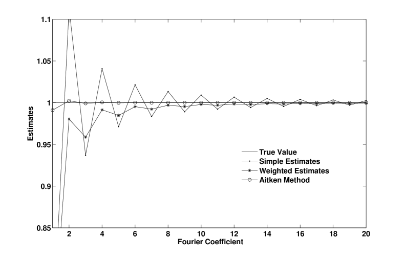
Figure 1: Performances of three type of estimates: Simple, Weighted Averages and Aitken’s $\triangle^{2}$ method

4 Closed-form Exact Estimators

In regular models, the estimator is consistent in the large sample or small noise limit; neither of these limits can be evaluated exactly from any actual observations. In singular models, there often exists an estimator that is consistent in the limit that can potentially be evaluated exactly from the available observations. Still, no expression can be evaluated on a computer unless the expression involves only finitely many operations of addition, subtraction, multiplication, and division.

Definition 4.1.

An estimator is called closed-form exact if it produces the exact value of the unknown parameter after a finite number of additions, subtractions, multiplications, and divisions performed on the elementary functions of the observations.

Closed-form exact estimators exist for the model (3.1) if we assume that the observations are $u_{k}(t),\ k\geq 1,\ t\in[0,T]$.

As an illustration, consider the simple example

$$du-\theta u_{xx}dt=(u/2)dt+udW(t),$$

where $x\in(0,\pi)$ and zero boundary conditions are assumed.

With $h_{k}=\sqrt{2/\pi}\,\sin(kx)$, we find

$$du_{k}(t)=-k^{2}\theta u_{k}(t)dt+(u_{k}/2)dt+u_{k}(t)dW(t).$$

Set $v_{k}(t)=\ln(u_{k}(t)/u_{k}(0))$. Then

$$dv_{k}(t)=-k^{2}\theta dt+dW(t).$$

In particular,

$$v_{1}(T)=-\theta T+W(T),\ v_{2}(T)=-4\theta T+W(t)$$

so that

$$\theta=\frac{v_{1}(T)-v_{2}(T)}{3T}$$

or

$$\theta=\frac{1}{3T}\ln\frac{u_{1}(T)u_{2}(0)}{u_{1}(0)u_{2}(T)}.$$ (4.1)

Notice that given $u_{1},\ldots,u_{N}$, we have $N(N-1)/2$ exact estimators of this type.

If there are two Wiener processes driving the equation, then we will need three different $u_{k}$ to construct an estimator of the type (4.1). The general result is as follows.

Theorem 4.2.

In addition to conditions of Theorem 3.1 assume that there exist two finite sets of indices $(k_{1}^{i},k_{2}^{i},\ldots,k_{n}^{i}),\ i=1,2$, and a positive integer $p$ such that

$$\sum_{\ell=1}^{n}\nu_{k_{\ell}^{1}}\mu_{pk_{\ell}^{2}}\neq\sum_{\ell=1}^{n}\nu_{k_{\ell}^{2}}\mu_{pk_{\ell}^{1}}.$$

Then there exists a closed-form exact estimator for $\theta$.

Proof.

Let $v_{k}(t)=\ln(u_{k}(t)/u_{k}(0))$. From (3.3), by Itô’s formula, we get

$$dv_{k}=-\Big{(}\rho_{k}+\theta\nu_{k}+\frac{1}{2}M_{k}\Big{)}dt+\sum\limits_{j\geq 1}\mu_{jk}dW_{j}(t),$$ (4.2)

and then

$$\begin{split}\theta\sum_{\ell=1}^{n}\Big{(}\nu_{k_{\ell}^{2}}\mu_{pk_{\ell}^{1}}-\nu_{k_{\ell}^{1}}\mu_{pk_{\ell}^{2}}\Big{)}&=\frac{1}{T}\sum_{\ell=1}^{n}\Big{(}\mu_{pk_{\ell}^{2}}v_{k_{\ell}^{1}}(T)-\mu_{pk_{\ell}^{1}}v_{k_{\ell}^{2}}(T)\\ &+\mu_{pk_{\ell}^{2}}(\rho_{k_{\ell}^{1}}+\frac{1}{2}M_{k_{\ell}^{1}})-\mu_{pk_{\ell}^{1}}(\rho_{k_{\ell}^{2}}+\frac{1}{2}M_{k_{\ell}^{2}})\Big{)},\end{split}$$ (4.3)

which completes the proof. ∎

If there are $n_{0}$ Wiener processes driving the equation, then the extra condition of the theorem can always be ensured with $n=n_{0}+1$, because every collection of $n$ vectors in an $n-1$-dimensional space is linearly dependent. While relation (4.3) gives a closed-form exact estimator, the resulting formulas can be rather complicated when the number of Wiener processes in the equation is large; if this number is infinite, then the estimator might not exist at all. For comparison, the complexity of the maximum likelihood estimator (3.7) does not depend on the number of Wiener processes in the equation. As a result, when it comes to actual computations, the closed-form exact estimator is not necessarily the best choice. On the other hand, the very existence of such an estimator is rather remarkable.

We conclude this section with three examples of closed-form exact estimators. The first example shows that such estimators can exist for equations that are not diagonalizable in the sense of Definition 2.1.

Example 3.

Consider the equation

$$du(t,x)=\theta u_{xx}(t,x)dt+u(t,x)dW(t),\ 0<t\leq T,\ x\in\mathbb{R}.$$

By the Itô formula,

$$u(t,x)=v(t,x)\exp(W(t)-(t/2)),$$

where $v$ solves the heat equation $v_{t}=\theta v_{xx}$, $v(0,x)=u(0,x)$. Assume that $u(0,x)$ is a smooth compactly supported function. Then $u(t,x)$ is a smooth bounded function for all $t>0,x\in\mathbb{R}$ and $\mathbb{E}\int_{\mathbb{R}}|u(t,x)|^{p}dx<\infty$ for all $p>0$, $t\geq 0$. In particular, the Fourier transform $U(t,y)$ of $u$ is defined and satisfies

$$dU(t,y)=-\theta y^{2}U(t,y)dt+U(t,y)dW(t).$$

Let $V(t)=\ln(U(t)/U(0))$. Then

$$V(T,y)=-y^{2}\theta T-(T/2)+W(T),$$

and

$$\theta=\frac{V(T,y_{1})-V(T,y_{2})}{T(y_{2}^{2}-y_{1}^{2})}.$$

The next example shows that conditions (2.3) and (3.10) are not related to the existence of a closed-form exact estimator.

Example 4.

Consider the equation

$$du-(\boldsymbol{\Delta}u+\theta u)dt=(I-\boldsymbol{\Delta})^{3/4}udW(t)$$

on $(0,\pi)$ with zero boundary conditions. Clearly both (2.3) and (3.10) are not satisfied. While the equation is not parabolic, there exists a unique solution in weighted Wiener chaos spaces, and we can therefore consider

$$du_{k}=(-k^{2}u_{k}+\theta u_{k})dt-(1+k^{2})^{3/4}u_{k}dW(t).$$

For $v_{k}(t)=\ln(u_{k}(t)/u_{k}(0))$ we find

$$v_{k}(T)=(-k^{2}-\frac{(1+k^{2})^{3/2}}{2})T+\theta T+(1+k^{2})^{3/4}W(t).$$

In particular,

$$v_{1}(T)=a_{1}T+b_{1}W(t)+\theta T,\ v_{2}(T)=a_{2}T+b_{2}W(T)+\theta T,$$

and so

$$\theta=\frac{b_{1}v_{2}(T)-b_{2}v_{1}(T)-(a_{2}b_{1}-a_{1}b_{2})T}{T(b_{1}-b_{2})}.$$

The last example shows that, as long as there is no spacial structure in the noise, multiplicativity of the noise is not necessary to have a closed-form exact estimator.

Example 5.

Consider the equation

$$du(t,x)=\theta u_{xx}(t,x)dt+dW(t),t>0,\ x\in(0,\pi),$$

with Neumann boundary conditions, so that $h_{1}=1/\sqrt{\pi}$ and $h_{k}=\sqrt{2/\pi}\cos((k-1)x)$, $k\geq 2$. Then $du_{2}(t)=-\theta u_{2}(t)dt$, and, as long as $u_{2}(0)\not=0$, we have

$$\theta=\frac{1}{T}\ln\frac{u_{2}(0)}{u_{2}(T)}.$$

References

• [1] S. I. Aihara (1992) Regularized maximum likelihood estimate for an infinite-dimensional parameter in stochastic parabolic systems, SIAM J. Control Optim. 30(4):745–764.
• [2] A. Bagchi and V. Borkar (1984) Parameter identification in infinite-dimensional linear systems, Stochastics 12(3-4):201–213.
• [3] R. Cont (2005) Modeling term structure dynamics: an infinite dimensional approach, Int. J. Theor. Appl. Finance 8(3):357–380.
• [4] C. Frankignoul (2000) Sst anomalies, planetary waves and rc in the middle rectitudes, Reviews of Geophysics 30(7):1776–1789.
• [5] J. Gáll, G. Pap, M. C. A. van Zuijlen (2006) Forward interest rate curves in discrete time settings driven by random fields, Comput. Math. Appl. 51(3-4):387–396.
• [6] R. S. Goldstein (2000) The term structure of interest rates as random field, Review of Financial Studies (13):365–384.
• [7] M. Huebner, S. Lototsky, B. L. Rozovskii (1997) Asymptotic properties of an approximate maximum likelihood estimator for stochastic PDEs, Statistics and control of stochastic processes (Moscow, 1995/1996), World Sci. Publishing, pp139–155.
• [8] M. Huebner, B. Rozovskii, R. Khasminskii (1992) Two examples of parameter estimation, In:Stochastic Processes, ed. Cambanis, Chos, Karandikar, Berlin, Springer.
• [9] M. Huebner, B. L. Rozovskiĭ (1995) On asymptotic properties of maximum likelihood estimators for parabolic stochastic PDE’s, Probab. Theory Related Fields 103(2):143–163.
• [10] I. A. Ibragimov, R. Z. Khasminskiĭ (1981) Statistical estimation, Applications of Mathematics, vol. 16, Springer-Verlag, New York.
• [11] I. A. Ibragimov, R. Z. Khasminskiĭ (1998) Problems of estimating the coefficients of stochastic partial differential equations. I, Teor. Veroyatnost. i Primenen. 43(3):417–438.
• [12] I. A. Ibragimov, R. Z. Khasminskiĭ (1999) Problems of estimating the coefficients of stochastic partial differential equations. II, Teor. Veroyatnost. i Primenen. 44(3):526–554.
• [13] I. A. Ibragimov, R. Z. Khasminskiĭ (2000) Problems of estimating the coefficients of stochastic partial differential equations. III, Teor. Veroyatnost. i Primenen. 45(2):209–235.
• [14] R. Khasminskii, N. Krylov, N. Moshchuk (1999) On the estimation of parameters for linear stochastic differential equations, Probab. Theory Related Fields 113(3):443–472.
• [15] S. G. Kreĭn, Yu. Ī. Petunīn, E. M. Semënov (1982) Interpolation of linear operators, Translations of Mathematical Monographs, vol. 54, American Mathematical Society, Providence, R.I.
• [16] R. S. Liptser, A. N. Shiryayev (2000) Statistics of random processes I. General theory, 2nd ed., Springer-Verlag, New York.
• [17] S. V. Lototsky (2003) Parameter estimation for stochastic parabolic equations: asymptotic properties of a two-dimensional projection-based estimator, Stat. Inference Stoch. Process. 6(1):65–87.
• [18] S. V. Lototsky, B. L. Rozovskii (1999) Spectral asymptotics of some functionals arising in statistical inference for SPDEs, Stochastic Process. Appl. 79(1):69–94.
• [19] S. V. Lototsky, B. L. Rozovskii (2000) Parameter estimation for stochastic evolution equations with non-commuting operators, In:Skorohod’s Ideas in Probability Theory, V.Korolyuk, N.Portenko and H.Syta (ed), Institute of Mathematics of National Academy of Sciences of Ukraine, Kiev, Ukraine, 2000, pp271–280.
• [20] S. V. Lototsky, B. L. Rozovskii (2006) Wiener chaos solutions of linear stochastic evolution equations, Ann. Probab. 34(2):638–662.
• [21] L. I. Piterbarg (2001/02) The top Lyapunov exponent for a stochastic flow modeling the upper ocean turbulence, SIAM J. Appl. Math. 62(3):777–800 (electronic).
• [22] L. I. Piterbarg (2005) Relative dispersion in 2D stochastic flows, J. Turbul. 6 (2005), Paper 4 (electronic).
• [23] L. I. Piterbarg, B. L. Rozovskii (1997) On asymptotic problems of parameter estimation in stochastic PDE’s: discrete time sampling, Math. Methods Statist. 6(2):200–223.
• [24] B. L. Rozovskii (1990) Stochastic evolution systems, Mathematics and its Applications (Soviet Series), vol. 35, Kluwer Academic Publishers Group, Dordrecht, Linear theory and applications to nonlinear filtering.
• [25] S. E. Serrano, T. E. Unny (1990) Random evolution equations in hydrology, Appl. Math. Comput. 38(3):201–226.
• [26] M. A. Shubin (2001) Pseudodifferential operators and spectral theory, second ed., Springer-Verlag, Berlin.
• [27] J. B. Walsh (1986) An introduction to stochastic partial differential equations, École d’été de probabilités de Saint-Flour, XIV—1984, Lecture Notes in Math., vol. 1180, Springer, Berlin, 1986, pp265–439.