New UltraCool and Halo White Dwarf Candidates in SDSS Stripe 82

Abstract

A $2.5^{\circ}\times 100^{\circ}$ region along the celestial equator (Stripe 82) has been imaged repeatedly from 1998 to 2005 by the Sloan Digital Sky Survey. A new catalogue of $\sim 4$ million light-motion curves, together with over 200 derived statistical quantities, for objects in Stripe 82 brighter than $r\sim 21.5$ has been constructed by combining these data by Bramich et al. (2007). This catalogue is at present the deepest catalogue of its kind. Extracting the $\sim 130\,000$ objects with highest signal-to-noise ratio proper motions, we build a reduced proper motion diagram to illustrate the scientific promise of the catalogue. In this diagram disk and halo subdwarfs are well-separated from the cool white dwarf sequence. Our sample of 1049 cool white dwarf candidates includes at least 8 and possibly 21 new ultracool H-rich white dwarfs (${T_{\rm eff}}<4000$ K) and one new ultracool He-rich white dwarf candidate identified from their SDSS optical and UKIDSS infrared photometry. At least 10 new halo white dwarfs are also identified from their kinematics.

1 Introduction

The number of detected cool white dwarfs has risen dramatically with the advent of the deep all-sky surveys, like the Sloan Digital Sky Survey (SDSS). Nonetheless, certain classes of white dwarfs – for example, ultracool white dwarfs and halo white dwarfs – remain intrinsically scarce.

The first ultracool (${T_{\rm eff}}<4000$ K) white dwarfs were discovered by Harris et al. (1999) and Hodgkin et al. (2000). Molecular hydrogen in their atmospheres causes a high opacity at infrared wavelengths, producing a spectral energy distribution with depleted infrared flux (e.g., Harris et al., 1999; Bergeron & Leggett, 2002). Six ultracool white dwarfs have already been found in the SDSS on the basis of their unusual colours and spectral shape (Harris et al., 2001; Gates et al., 2004). Recently, Kilić et al. (2006) used a combination of SDSS photometry and United States Naval Observatory ‘B’ (USNO-B) astrometry to double the still tiny sample of these interesting objects, which probe the earliest star formation in the Galactic disk.

The halo white dwarfs are of astronomical interest as probes of the earliest star formation in the proto-Galaxy, and as tests of the age of the oldest stars. Liebert et al. (1998) first identified six candidate halo white dwarfs on the basis of high proper motions. Subsequently, Oppenheimer et al. (2001) claimed the discovery of 38 high proper motion white dwarfs, but it is unclear whether they are halo or thick disk members (Reid et al., 2001). Harris et al. (2006) recently identified a sample of $\sim 6000$ cool white dwarfs from SDSS Data Release 3 (DR3) using reduced proper motions, based on SDSS and USNO-B combined data (Munn et al., 2004). The sample included 33 objects with substantial tangential velocity components ($>$ 160 kms^-1) and so are excellent halo white dwarf candidates.

In this paper, we also use SDSS data to identify new members of the cool white dwarf population. SDSS Stripe 82 is a $2.5^{\circ}\times 100^{\circ}$ strip along the celestial equator which has been repeatedly imaged between 1998 and 2005. We exploit the new catalogue of almost four million light-motion curves in Stripe 82 (Bramich et al., 2007). By extracting the subset of $\sim 130\,000$ objects with high signal-to-noise ratio proper motions, we build a clean reduced proper motion diagram, from which we identify 1049 cool white dwarfs up to a magnitude $r\sim 21.5$. Further diagnostic information is obtained by combining the catalogue with near-infrared photometry from the UKIRT Infrared Digital Sky Survey (UKIDSS) Data Release 2 (DR2) (Warren et al., 2007b). This enables us to present new, faint samples of the astronomically important ultracool white dwarfs and halo white dwarfs.

Figure 1: Measured proper motion in RA (track at bottom left, left-hand y-scale) and Dec (track at top left, right-hand y-scale) for the ultracool white dwarf candidate SDSS J224845.93–005407.0.

2 SDSS and UKIDSS Data on Stripe 82

SDSS is an imaging and spectroscopic survey (York et al., 2000) that has mapped more than a quarter of the sky. Imaging data are produced simultaneously in five photometric bands, namely $u$, $g$, $r$, $i$, and $z$ (Fukugita et al., 1996; Gunn et al., 1998; Hogg et al., 2001; Adelman-McCarthy et al., 2006; Gunn et al., 2006; Adelman-McCarthy et al., 2007). The data are processed through pipelines to measure photometric and astrometric properties (Lupton, Gunn, & Szalay, 1999; Stoughton et al., 2002; Smith et al., 2002; Pier et al., 2003; Ivezić et al., 2004; Tucker et al., 2006).

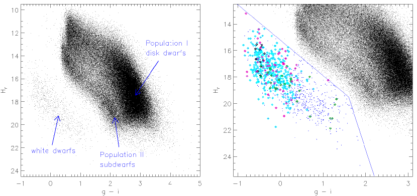
Figure 2: Left: Reduced proper motion (RPM) diagram for Stripe 82. Plotted magnitudes are inverse-variance weighted mean light curve magnitudes without any correction for reddening. The sequences corresponding to white dwarfs, Population I disk dwarfs, and Population II main sequence subdwarfs are well distinguishable. Right: Zoom on the white dwarf region of the RPM diagram. The thin blue line separates the white dwarfs (blue dots on the left) from the dwarf and subdwarf populations (black dots on the right). Previously spectroscopically confirmed white dwarfs are also shown: WDs of spectral type DA (338 in total) as cyan diamonds, WDs of spectral type DB (12 in total) as black diamonds, WDs of spectral type DC (29 in total) as green diamonds and WDs of any other spectral type (50 in total) as magenta diamonds (Harris et al., 2003; McCook & Sion, 2003; Kleinman et al., 2004; Carollo et al., 2006; Eisenstein et al., 2006; Kilić et al., 2006; Silvestri et al., 2006).

SDSS Stripe 82 covers a $\sim 250$ deg² area of sky, consisting of a $2.5^{\circ}$ strip along the celestial equator from right ascension $-49.5^{\circ}$ to $+49.5^{\circ}$. The stripe has been repeatedly imaged between June and December each year from 1998 to 2005. Sixty-two of the total of 134 available imaging runs were obtained in 2005. This multi-epoch 5-filter photometric data set has been utilised by Bramich et al. (2007) to construct the Light-Motion-Curve Catalogue (LMCC) and the Higher-Level Catalogue (HLC). The LMCC contains 3 700 548 light-motion curves, extending to magnitude 21.5 in $u$, $g$, $r$, $i$ and to magnitude 20.5 in $z$. A typical light-motion curve consists of $\simeq$30 epochs over a baseline of 6–7 years. The root-mean-square (RMS) scatter in the individual position measurements is $23\,\mathrm{mas}$ in each coordinate for $r\leq 19.0$, increasing exponentially to $60\,\mathrm{mas}$ at $r=21.0$ (Bramich et al., 2007). The HLC includes 235 derived quantities, such as mean magnitudes, photometric variability parameters and proper-motion, for each light-motion curve in the LMCC. As an illustration of the catalogue’s potential, Fig. 1 shows a measured proper motion in RA and Dec for SDSS J224845.93–005407.0, one of the ultracool white dwarf candidates extracted from the LMCC. The source is faint ($r=20.56$) and has a measured proper-motion of $204\pm 5\,\mathrm{mas}\,\mathrm{yr^{-1}}$.

UKIDSS is the UKIRT Infrared Deep Sky Survey (Lawrence et al., 2007; Hewett et al., 2006; Irwin et al., 2007; Hambly et al., 2007), carried out using the Wide Field Camera (Casali et al., 2007) installed on the United Kingdom Infrared Telescope (UKIRT). The survey is now well underway with three ESO-wide releases: the Early Data Release (EDR) in February 2006 (Dye et al., 2006), the Data Release 1 (DR1) in July 2006 (Warren et al., 2007a) and the Data Release 2 in March 2007 (Warren et al., 2007b). In fact UKIDSS is made up of five surveys. The UKIDSS Large Area Survey (LAS) is a near-infrared counterpart of the SDSS photometric survey. The UKIDSS DR2 (Warren et al., 2007b) provides partial coverage, consisting of observations in at least one of $YJHK$-bands (Hewett et al., 2006), of $\sim 2/3$ of Stripe 82 to a depth of $K\simeq 20.1$.

3 Data Analysis

3.1 A Reduced Proper Motion Diagram

The reduced proper motion (RPM) is defined as $H=m+5\log\mu+5$, where $m$ is the apparent magnitude and $\mu$ is the proper motion in arcseconds per year. Recently, Kilić et al. (2006) have combined the SDSS Data Release 2 (DR2) and the USNO–B catalogues, using the resulting distribution of RPMs as a tracer of cool white dwarfs. Here, our HLC for Stripe 82 enables us to construct an RPM diagram using only SDSS data. Magnitudes used in the RPM diagram are mean magnitudes, calculated from all available single epoch SDSS measurements. These values therefore differ from magnitudes quoted in the publicly available SDSS database which are based on a single photometric measurement. Differences are usually small, of the order of some hundredths of a magnitude. Typical proper motion errors in right ascension and declination are $\sim 2\,\mathrm{mas\,yr^{-1}}$ for $r\sim 17$ and $\sim 3\,\mathrm{mas\,yr^{-1}}$ for $r\sim 21$ which is slightly better than that of Kilić et al. (2006) despite the much shorter time baseline used for calculating proper motions in the HLC. Additionally, the shorter time baseline with many position measurements has the advantage of reducing the contamination due to mismatches of objects with larger proper motions. The Stripe 82 photometric catalogue extends approximately $1.5$ mag deeper than the SDSS-DR2/USNO-B catalogue, corresponding to a factor of two in distance. Taking into account the different sky coverage of the two catalogues, the resultant volume over which white dwarfs may be detected in the HLC is $\simeq 60\,$per cent of that accessible in the SDSS-DR2/USNO-B catalogue.

In the left panel of Fig. 2, we present the RPM diagram for all 131 398 objects in Stripe 82 that meet the following criteria: i) the light curve consists of at least nine epochs in the $g$, $r$, $i$ and $z$ filters, ii) the object is classified as stellar by the SDSS photometric analysis in at least 80 per cent of the epochs, iii) the proper motion is measured with a $\mathrm{\sqrt{\Delta\chi^{2}}}\geq 9$. In the case of high proper motion objects ($\mu\geq 50\ \mathrm{mas}\ \mathrm{yr^{-1}}$), the latter requirement is relaxed to allow a $\mathrm{\sqrt{\Delta\chi^{2}}}\geq 6$ measurement. The delta chi-squared $\Delta\chi^{2}$ of the proper motion fit is defined as:

$$\Delta\chi^{2}=\chi^{2}_{\alpha,con}-\chi^{2}_{\alpha,lin}+\chi^{2}_{\delta,con}-\chi^{2}_{\delta,lin}\quad,$$ (1)

where $\chi^{2}_{con}$ is the chi-squared of the $\alpha/\delta$ measurements for a model that includes only a mean position and $\chi^{2}_{lin}$ is the chi-squared of the $\alpha/\delta$ measurements for a model that includes a mean position and a proper motion. This $\Delta\chi^{2}$ statistic follows a chi-square distribution with two degrees of freedom. A relatively high $\mathrm{\Delta\chi^{2}}$ threshold was adopted in order to keep distinct stellar populations in the RPM diagram cleanly separated.

The object sample was then matched with the UKIDSS DR2 catalogue using a search radius of 4$\aas@@fstack{\prime\prime}$0. Approximately 70 per cent of the sample had at least one near-infrared detection. The unmatched fraction results from a combination of the incomplete coverage of Stripe 82 in the UKIDSS DR2 and a proportion of the faintest SDSS objects possessing infrared magnitudes below the UKIDSS LAS detection limits.

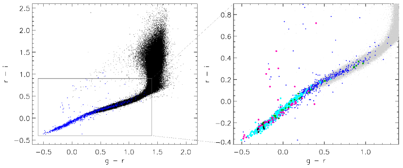
Figure 3: Left: Colour-colour diagrams for all the objects plotted in the left panel of Fig. 2. White dwarfs (candidates and confirmed) are overplotted as blue dots. The overlap between the cooler end of the white dwarf locus and the main sequence star locus is clearly seen. Right: Zoom on the white dwarf region of the colour-colour diagram. The main sequence star locus is this time plotted in a light grey colour. Spectroscopically confirmed white dwarfs are shown, using the same colour coding as in the right panel of Fig. 2. From this plot one can see that our new white dwarf candidates are typically cooler objects.

The left panel of Fig. 2 shows three distinct sequences of stars, namely Population I disk dwarfs, Population II main sequence subdwarfs and disk white dwarfs. Given that our primary target population consists of nearby white dwarfs, the magnitudes and colours used throughout the paper have not been corrected for the effects of Galactic reddening. Adopting a boundary between the subdwarfs and white dwarfs defined by $H_{r}>2.68\,(g-i)+15.21$ for $g-i\leq 1.6$ and $H_{r}>10.0\,(g-i)+3.5$ for $g-i>1.6$ produces a sample of 1049 candidate white dwarfs (see the right panel of Fig. 2). 446 of the white dwarf candidates possess at least one detection in the near-infrared UKIDSS DR2. The discrimination boundary is similar to that employed by Kilić et al. (2006) and lies in a sparsely populated region of the RPM diagram, where the individual magnitude and proper-motion errors are small. As a consequence, the population of white dwarfs is not too sensitive to the precise details of the separation boundary adopted. In this border region a small contamination from the subdwarfs is still possible (Kilić et al., 2006).

In the left panel of Fig. 3 we show the overlap in colour space between the cooler end of the white dwarf locus with the main sequence star locus. One can see that it is impossible to distinguish cooler white dwarfs from the main sequence stars based on colour information only and proper motions for these cool objects are needed. The effectiveness of our RPM selection is evident from the location of 429 spectroscopically confirmed white dwarfs from a number of sources (Harris et al., 2003; McCook & Sion, 2003; Kleinman et al., 2004; Carollo et al., 2006; Eisenstein et al., 2006; Kilić et al., 2006; Silvestri et al., 2006) in the right panels of Fig. 2 and Fig. 3. The previously confirmed white dwarfs populate practically only the upper half of the white dwarf sequence in the RPM diagram and the hotter end of the white dwarf locus in the colour-colour diagram. Confirmed cooler white dwarfs are rare and almost all originate from Kilić et al. (2006) where a similar detection method was adopted. The HLC is the faintest existing photometric/astrometric catalogue which enables us to trace hotter and thus intrinsically brighter white dwarfs to further distances and also to significantly enlarge the number of known cooler and thus intrinsically fainter white dwarfs.

Fig. 4 is a copy of the right panel of Fig. 2 with the model loci for pure H atmosphere white dwarfs overplotted (Bergeron et al., 2001). For clarity only loci for $\log g=8.0$ and $\log g=9.0$, using typical disk and halo tangential velocities ${V_{\rm T}}=30\,\mathrm{kms}^{-1}$ and ${V_{\rm T}}=160\,\mathrm{kms}^{-1}$ are shown. In reality the $\log g$ values for white dwarfs range from $\sim 7.0$ to $\sim 9.5$ and the tangential velocities in the disk span from $\sim 20\,\mathrm{kms}^{-1}$ to $\sim 40\,\mathrm{kms}^{-1}$ which results in a strong overlap between different model loci. Because of this degeneracy it is impossible to determine unique white dwarf physical properties only from their positions in the RPM diagram. In the colour-colour diagrams of Fig. 5 the model loci for pure H and He atmosphere white dwarfs are plotted for a range of log g values (Bergeron et al., 2001). White dwarfs for different $\log g$ values have very similar colours. Colour differences are well measurable only at the very cool end of the model tracks. This holds for white dwarfs with either H or He atmospheres. It is also not obviously feasible to distinguish between the H and He atmosphere white dwarfs. In some parts of the parameter space there is complete degeneracy.

3.2 $\chi^{2}$ Analysis

In order to compare the available magnitude information for each white dwarf candidate with the best matching model (Bergeron et al., 2001), a minimal normalised $\chi^{2}$ value was calculated:

$$\chi^{2}=\frac{1}{N}\sum_{i=1}^{N}\left(\frac{m_{i}-m(T_{eff},\log{g})_{i}-D}{m_{err,i}}\right)^{2}\quad,$$ (2)

where $m_{i}$ are measured magnitudes for a given object, $m(T_{eff},\log{g})_{i}$ its corresponding model predictions and $m_{err,i}$ measured magnitude errors. The best solution was sought on a grid of three free parameters, namely effective surface temperature ($T_{eff}$), surface gravity ($\log{g}$) and distance modulus ($D$). For each of the 1049 white dwarf candidates the four SDSS magnitudes, $g$, $r$, $i$ and $z$, were used in the fit. Whenever any of the UKIDSS magnitudes were available the fit was repeated with this additional information included. Only a small subset of 70 white dwarf candidates have as yet all three $J$, $H$ and $K$ UKIDSS magnitudes measured. Both H and He atmosphere models were compared with the data. In the attempt to better understand the degeneracy effects the best and also the second best solutions were recorded.

The statistical analysis of the obtained normalised $\chi^{2}$ results was performed first on the complete white dwarf sample, using only SDSS magnitude information. In all cases the $\chi^{2}$ distributions are strongly asymmetric. Typically fits of the H models perform better than the He ones. For the H models the normalised $\chi^{2}$ distribution peaks at $\sim 1.5$ and has a width of $\sim 3$ while for the He models the distribution peak is at $\sim 2.5$ and the width is $\sim 3.5$. Differences between the two fits are however usually too small to clearly distinguish between the two, especially in the temperature range where the H and He models are degenerate.

White dwarf atmosphere models observed in broad-band colours are also degenerate for different surface gravity values. In order to estimate how strongly this degeneracy affects the results of the fit we compared the calculated best normalised $\chi^{2}$ solutions with the second best ones. From the differences in the calculated $\chi^{2}$ values it is usually not possible to completely discard the second best solution. For instance, in the H model case, the second best normalised $\chi^{2}$ distribution peaks at $\sim 3$ with a distribution width of $\sim 3$. Nevertheless, for $\sim 60\,$per cent of the white dwarf candidates both best and second best solution predict the same effective temperature. For the remaining white dwarfs both temperatures usually differ from each other only by $\leq 5\,$per cent, which typically corresponds to two adjacent bins on the discrete grid of available models. Available photometric information is thus sufficient to reliably estimate the white dwarf effective temperature. Not surprisingly, the fit results of the surface gravity (and as a consequence also distance) are much less certain. The typical $\log{g}$ difference between the best and second best solution lies in the range from 0.5 to 1.5.

We used the subsample of 70 white dwarfs with complete UKIDSS photometry available to show how the UKIDSS data improve the constraints on the model fits. The normalised $\chi^{2}$ of the fit using the complete SDSS and UKIDSS magnitude information is typically smaller by 0.5 than the value from the fit using SDSS data only. In $85\,$per cent of the cases the temperature predictions are the same, otherwise the difference is only one step on the model temperature grid, which confirms the reliability of the temperature estimation. Moreover, in $85\,$per cent of the cases also the surface gravity solutions are the same and in the remaining $15\,$per cent of the cases the best SDSS+UKIDSS solution often corresponds to the second best SDSS solution. This might indicate that the UKIDSS data help in breaking the degeneracy in the $\log{g}$ parameter. When this is not the case, the normalised $\chi^{2}$ are always larger ($>10$). 70 white dwarfs is still too small a number to draw definite conclusions, however, it seems that the inclusion of the UKIDSS data significantly enhances the credibility of the photometric fits. This will be very important in the near future, when it will be possible to match large portions of the SDSS/USNO-B measurements with the rapidly increasing LAS UKIDSS database.

4 Candidates

4.1 Ultracool White Dwarfs

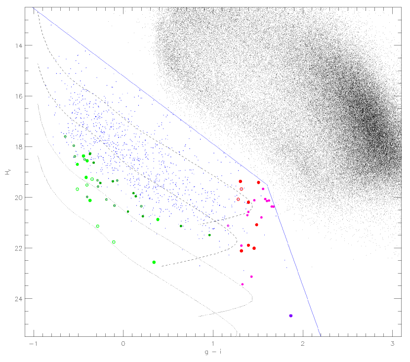
Figure 4: As in the right panel of Fig. 2 the zoom on the white dwarf region of the RPM diagram is shown. White dwarf H atmosphere models (Bergeron et al., 2001) for $\log g=8.0$ (upper of the dashed/dotted lines) and $\log g=9.0$ (lower of the dashed/dotted lines), using typical disk and halo tangential velocities ${V_{\rm T}}=30\,\mathrm{kms}^{-1}$ (dashed lines) and ${V_{\rm T}}=160\,\mathrm{kms}^{-1}$ (dotted lines) are overplotted. Larger red circles indicate H-rich ultracool white dwarf candidates, larger violet circles He-rich ultracool white dwarf candidates and smaller magenta circles possible H-rich ultracool white dwarf candidates (see detailed explanation in text). Halo white dwarf candidates are marked as light green larger circles and possible halo white dwarf candidates as dark green smaller circles (see detailed explanation in text). Empty circles of any colour mark objects that were already previously spectroscopically observed, full circles mark new detections.

The signature of an ultracool surface temperature (${T_{\rm eff}}<4000$ K) is depleted infrared flux, which makes the IR UKIDSS measurements crucial for the recognition of the ultracool white dwarf candidates. Unfortunately only a small subsample of the 1049 white dwarfs have at least one UKIDSS measurement available as yet. That is why we first examined the outcome of the H and He atmosphere model fits performed on the complete white dwarf sample, using SDSS magnitude information only. If the calculated surface temperature was smaller than $4000\,K$ and the normalised $\chi^{2}$ value of the fit was $<15$ the object was added to the ultracool white dwarf candidate list. In the subsample of white dwarfs with at least one UKIDSS measurement this additional piece of information was then used as a confirmation or rejection of potential ultracool white dwarf candidates. Typically the SDSS and UKIDSS predictions agreed.

The results of this analysis, graphically presented in Fig. 4 and Fig. 5, are the following:

• 9 ultracool white dwarf candidates with H-rich atmosphere among which 7 have at least one supportive UKIDSS measurement. The object SDSS J224206.19$+$004822.7 has already been spectroscopically confirmed as a DC type white dwarf (no strong spectral lines present, consistent with an H or He atmosphere) by Kilić et al. (2006) with a measured surface temperature of $\sim 3400\,$K. The object SDSS J233055.19$+$002852.2 has been spectroscopically confirmed also as a DC type white dwarf by the same authors. Its measured surface temperature is $\sim 4100\,$K which is just above the ultracool limit.

• One ultracool white dwarf candidate based on SDSS photometry only with He-rich atmosphere.

• 14 possible H-rich ultracool white dwarf candidates. For these candidates the fit of the He atmosphere model gives in fact a slightly better result, predicting as a consequence an object with not so extremely low surface temperature. Taking into account small differences between the H and He colours and the fact that H-rich white dwarfs are in fact much more numerous than the He-rich ones, makes these 14 objects still serious ultracool white dwarf candidates. The object SDSS J232115.67$+$010223.8 has been spectroscopically confirmed as a DC type white dwarf by Carollo et al. (2006). This object is also the only one where the fit based on only SDSS magnitudes did not predict an ultracool temperature but the inclusion of the UKIDSS K magnitude revealed the presence of the depleted IR flux. There are three additional ultracool candidates with at least one confirmed UKIDSS measurement.

Based on the positions in the RPM diagram and on the estimated tangential velocities, we conclude that the vast majority of the newly discovered ultracool white dwarf candidates are likely members of the disk population. Measured and calculated properties of the 24 ultracool white dwarf candidates are presented in Table 1. Due to the relatively large temperature errors, estimated to be at least $250\,K$ (the model temperature resolution in this temperature range), some of the 24 candidates might be in reality just above the ultracool white dwarf limit. We also do not quote the fit results for the surface gravity since these are as explained above too uncertain. It is possible that some of the new ultracool white dwarf candidates close to the adopted boundary are subdwarfs instead. All these open issues can be ultimately resolved only with spectroscopic follow up. However, already by analyzing the SDSS and UKIDSS astrometric/photometric information, it is certain that the total number of known ultracool white dwarfs has at least doubled.

4.2 Halo White Dwarfs

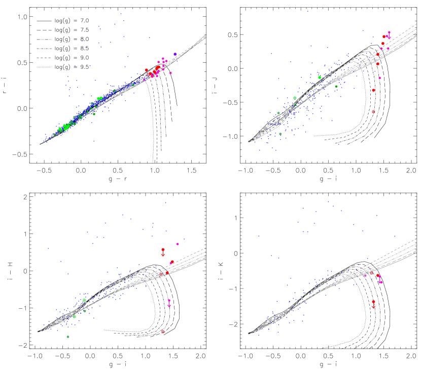
Figure 5: Colour-colour diagrams for all the white dwarfs selected from the RPM diagram. H and He atmosphere white dwarf models (Bergeron et al., 2001) for different surface gravity values are overplotted in black and grey respectively. Larger red circles indicate H-rich ultracool white dwarf candidates, larger violet circle He-rich ultracool white dwarf candidate and smaller magenta circles possible H-rich ultracool white dwarf candidates (see detailed explanation in text). The arrow indicates the limiting colour value for objects that were not detected in J, H or K respectively. Halo white dwarf candidates are marked as light green larger circles and possible halo white dwarf candidates as dark green smaller circles (see detailed explanation in text). Empty circles of any colour mark objects that were already previously spectroscopically observed, full circles mark new detections.

Harris et al. (2006) present a sample of 33 halo white dwarf candidates from their study employing the SDSS DR3 and USNO-B catalogues. The combination of their larger sky coverage and brighter magnitude limit of $r=19.7$ results in a survey volume three times that of our Stripe 82 survey.

Here we adopt the same criteria of ${V_{\rm T}}>160\,\mathrm{kms}^{-1}$ as Harris et al. (2006) to select halo white dwarf candidates using the results of the model fit. Unfortunately, white dwarf atmosphere models (Bergeron et al., 2001) are degenerate for different values of the $\log g$ parameter in a broad temperature range. This uncertainty in the calculation of the surface gravity is coupled with the determination of the distance to the object. Solutions with larger surface gravity and smaller distances are strongly coupled with those with smaller surface gravity and greater distance. As a consequence determination of the tangential velocity is also somewhat uncertain.

Therefore we divide our halo white dwarf candidates, presented in Table 2 and plotted in Fig. 4 and Fig. 5, into two groups:

• white dwarfs where the best and also second best fit solution indicate a quickly moving object. 12 highly probable halo candidates were thus found. Four were already previously spectroscopically observed (Kleinman et al., 2004; Eisenstein et al., 2006) and two of them, namely SDSS J010207.24$-$003259.7 and SDSS J234110.13$+$003259.5 were already included on the Harris et al. (2006) halo candidate list.

• white dwarfs where the best fit solution gives ${V_{\rm T}}>160\,\mathrm{kms}^{-1}$ but the second best fit solution does not. 22 white dwarfs were thus found and very likely not all of them are halo white dwarfs. 12 were already previously spectroscopically observed by (McCook & Sion, 2003; Kleinman et al., 2004; Eisenstein et al., 2006)

One of the ultracool white dwarf candidates, SDSS J030144.09$-$004439.5 has its calculated tangential velocity just below the threshold limit and could be thus also a member of the halo population.

5 Conclusions

Bramich et al. (2007) used the multi-epoch SDSS observations of Stripe 82 to build the deepest (complete to $r=21.5$) photometric/astrometric catalogue ever constructed, covering $\sim 250$ deg² of the sky. Here, we have exploited the catalogue to find new candidate members of scarce white dwarf sub-populations. We extracted the stellar objects with high signal-to-noise ratio proper motions and built a RPM diagram. Cleanly separated from the subdwarf populations in the RPM diagram are 1049 cool white dwarf candidates.

Amongst these, we identified at least 7 new ultracool H-rich white dwarf candidates, in addition to one already spectroscopically confirmed by Kilić et al. (2006) and one new ultracool He-rich white dwarf candidate . The effective temperatures ${T_{\rm eff}}$ of these eight candidates are all $<$4000 K. We also identified at least 10 new halo white dwarf candidates with a tangential velocity of ${V_{\rm T}}>160\,\mathrm{kms}^{-1}$. Spectroscopic follow-up of the new discoveries is underway.

In the quest for new members of still rare white dwarf sub-populations precise kinematic information and even more the combination of SDSS and UKIDSS photometric measurements will play an important role, as we illustrate here. For the ultracool white dwarfs near IR UKIDSS measurements turn out to be essential for making reliable identifications. In the near future the UKIDSS LAS will cover large portions of the sky imaged previously by SDSS. This gives bright prospects for an even more extensive search for the still very scarce ultracool white dwarfs.

Table 1:

Properties of the Ultracool White Dwarf Candidates

Object	$g$		$r$		$i$		$z$		$J$		$H$		$K$		$\mu$		$\varphi_{\mu}$	$D$	$V_{T}$	$T_{eff}$	$\chi^{2}$	type
SDSS J	[AB]		[AB]		[AB]		[AB]		[AB]†		[AB]†		[AB]†		[mas yr-1]		[degree]	[pc]	[km s-1]	[K]	SDSS
001107.57$-$003102.8	$21.68$$\,\pm\,$	$0.01$	$20.62$$\,\pm\,$	$0.01$	$20.17$$\,\pm\,$	$0.01$	$19.87$$\,\pm\,$	$0.02$	$19.71$$\,\pm\,$	$0.11$					$57$$\,\pm\,$	$5$	$126$	125	34	3750	5.3	H
004843.28$-$003820.0	$22.55$$\,\pm\,$	$0.03$	$21.44$$\,\pm\,$	$0.02$	$20.97$$\,\pm\,$	$0.01$	$20.53$$\,\pm\,$	$0.04$	$20.68$$\,\pm\,$	$0.28$	$20.25$$\,\pm\,$	$0.28$			$53$$\,\pm\,$	$9$	$163$	165	42	3500	8.5	H/He
012102.99$-$003833.6	$20.74$$\,\pm\,$	$0.01$	$19.75$$\,\pm\,$	$0.01$	$19.35$$\,\pm\,$	$0.01$	$19.17$$\,\pm\,$	$0.01$	$19.14$$\,\pm\,$	$0.08$	$19.40$$\,\pm\,$	$0.09$	$19.98$$\,\pm\,$	$0.19$	$123$$\,\pm\,$	$5$	$67$	55	32	3750	2.0	H
013302.17$+$010201.3	$22.74$$\,\pm\,$	$0.04$	$21.62$$\,\pm\,$	$0.02$	$21.11$$\,\pm\,$	$0.02$	$20.56$$\,\pm\,$	$0.06$							$50$$\,\pm\,$	$9$	$272$	175	41	3500	11.4	H/He
030144.09$-$004439.5	$20.45$$\,\pm\,$	$0.01$	$19.41$$\,\pm\,$	$0.01$	$19.02$$\,\pm\,$	$0.01$	$18.81$$\,\pm\,$	$0.01$	$19.16$$\,\pm\,$	$0.09$	$>19.81^{{\ddagger}}$		$>19.68^{{\ddagger}}$		$557$$\,\pm\,$	$3$	$169$	60	159	3750	9.0	H/He
204332.97$+$011436.2	$22.72$$\,\pm\,$	$0.04$	$21.56$$\,\pm\,$	$0.02$	$21.05$$\,\pm\,$	$0.02$	$20.49$$\,\pm\,$	$0.07$							$58$$\,\pm\,$	$13$	$122$	175	48	3500	8.9	H/He
205010.17$+$003233.7	$21.61$$\,\pm\,$	$0.04$	$20.72$$\,\pm\,$	$0.06$	$20.30$$\,\pm\,$	$0.10$	$19.89$$\,\pm\,$	$0.06$							$54$$\,\pm\,$	$12$	$193$	105	27	3750	1.4	H
205132.05$+$000353.6	$20.92$$\,\pm\,$	$0.02$	$19.64$$\,\pm\,$	$0.02$	$19.05$$\,\pm\,$	$0.02$	$18.57$$\,\pm\,$	$0.03$							$1016$$\,\pm\,$	$13$	$179$	20	88	3750	13.1	He
210742.26$-$002354.1	$22.33$$\,\pm\,$	$0.03$	$21.21$$\,\pm\,$	$0.01$	$20.79$$\,\pm\,$	$0.01$	$20.55$$\,\pm\,$	$0.05$							$82$$\,\pm\,$	$10$	$132$	125	49	3500	1.9	H/He
212216.01$-$010715.2	$21.72$$\,\pm\,$	$0.02$	$20.76$$\,\pm\,$	$0.01$	$20.41$$\,\pm\,$	$0.01$	$20.20$$\,\pm\,$	$0.04$							$170$$\,\pm\,$	$8$	$171$	65	51	3750	5.3	H/He
212930.25$-$003411.5	$21.24$$\,\pm\,$	$0.01$	$20.28$$\,\pm\,$	$0.01$	$19.91$$\,\pm\,$	$0.01$	$19.72$$\,\pm\,$	$0.02$							$428$$\,\pm\,$	$5$	$180$	50	102	3750	8.5	H/He
214108.42$+$002629.5	$22.81$$\,\pm\,$	$0.04$	$21.70$$\,\pm\,$	$0.02$	$21.16$$\,\pm\,$	$0.02$	$20.64$$\,\pm\,$	$0.06$							$54$$\,\pm\,$	$11$	$178$	180	47	3500	10.2	H/He
220455.03$-$001750.6	$21.58$$\,\pm\,$	$0.02$	$20.55$$\,\pm\,$	$0.01$	$20.20$$\,\pm\,$	$0.01$	$19.98$$\,\pm\,$	$0.02$							$107$$\,\pm\,$	$6$	$188$	80	41	3750	7.1	H/He
223105.29$+$004941.9	$21.84$$\,\pm\,$	$0.01$	$20.81$$\,\pm\,$	$0.01$	$20.36$$\,\pm\,$	$0.01$	$20.11$$\,\pm\,$	$0.03$	$19.99$$\,\pm\,$	$0.12$	$20.11$$\,\pm\,$	$0.17$			$114$$\,\pm\,$	$5$	$233$	140	74	3750	7.3	H
223520.19$-$003623.6	$22.17$$\,\pm\,$	$0.02$	$21.16$$\,\pm\,$	$0.01$	$20.77$$\,\pm\,$	$0.01$	$20.53$$\,\pm\,$	$0.04$	$20.71$$\,\pm\,$	$0.28$					$140$$\,\pm\,$	$6$	$81$	105	69	3750	1.6	H
223715.32$-$002939.2	$22.28$$\,\pm\,$	$0.03$	$21.07$$\,\pm\,$	$0.01$	$20.69$$\,\pm\,$	$0.01$	$20.48$$\,\pm\,$	$0.04$			$>20.15$				$65$$\,\pm\,$	$7$	$122$	110	34	3250	9.6	H/He
223954.07$+$001849.2	$20.99$$\,\pm\,$	$0.05$	$19.94$$\,\pm\,$	$0.02$	$19.53$$\,\pm\,$	$0.01$	$19.41$$\,\pm\,$	$0.02$	$19.24$$\,\pm\,$	$0.06$	$19.33$$\,\pm\,$	$0.10$	$20.36$$\,\pm\,$	$0.27$	$108$$\,\pm\,$	$4$	$352$	55	28	3500	0.5	H/He
224206.19$+$004822.7a	$19.61$$\,\pm\,$	$0.01$	$18.64$$\,\pm\,$	$0.01$	$18.30$$\,\pm\,$	$0.01$	$18.19$$\,\pm\,$	$0.01$	$18.94$$\,\pm\,$	$0.05$	$19.94$$\,\pm\,$	$0.15$	$>19.70$		$161$$\,\pm\,$	$4$	$117$	20	17	3500	2.6	H
224845.93$-$005407.0	$21.50$$\,\pm\,$	$0.01$	$20.56$$\,\pm\,$	$0.01$	$20.19$$\,\pm\,$	$0.01$	$19.98$$\,\pm\,$	$0.02$	$20.51$$\,\pm\,$	$0.21$	$>19.64$				$204$$\,\pm\,$	$5$	$112$	70	70	3750	1.3	H
225244.51$+$000918.6	$21.92$$\,\pm\,$	$0.02$	$20.91$$\,\pm\,$	$0.01$	$20.53$$\,\pm\,$	$0.01$	$20.28$$\,\pm\,$	$0.05$							$86$$\,\pm\,$	$8$	$33$	120	49	3750	4.1	H/He
232115.67$+$010223.8b	$19.81$$\,\pm\,$	$0.01$	$18.96$$\,\pm\,$	$0.01$	$18.65$$\,\pm\,$	$0.01$	$18.49$$\,\pm\,$	$0.01$					$19.28$$\,\pm\,$	$0.12$	$271$$\,\pm\,$	$6$	$201$	20	28	4250	8.3	H/He
233055.19$+$002852.2c	$19.89$$\,\pm\,$	$0.01$	$18.98$$\,\pm\,$	$0.01$	$18.61$$\,\pm\,$	$0.01$	$18.46$$\,\pm\,$	$0.01$			$18.70$$\,\pm\,$	$0.06$	$19.18$$\,\pm\,$	$0.09$	$166$$\,\pm\,$	$4$	$57$	25	21	3750	11.2	H
233818.56$-$004146.2	$22.27$$\,\pm\,$	$0.02$	$21.24$$\,\pm\,$	$0.01$	$20.81$$\,\pm\,$	$0.01$	$20.44$$\,\pm\,$	$0.04$							$142$$\,\pm\,$	$7$	$166$	165	112	3750	3.3	H
234646.06$-$003527.6	$22.52$$\,\pm\,$	$0.03$	$21.46$$\,\pm\,$	$0.02$	$20.96$$\,\pm\,$	$0.01$	$20.53$$\,\pm\,$	$0.04$	$20.48$$\,\pm\,$	$0.18$					$44$$\,\pm\,$	$7$	$170$	165	34	3500	8.7	H/He
a DC type white dwarf with $T_{eff}\simeq 3400\,$K (Kilić et al., 2006).
b DC type white dwarf (Carollo et al., 2006).
c DC type white dwarf with $T_{eff}\simeq 4100\,$K (Kilić et al., 2006).
† The UKIDSS Vega magnitudes are converted to the AB system adopting a magnitude for Vega of +0.03 and the passband zero-point offsets from Hewett et al. (2006).
‡ 5$\sigma$ magnitude detection limit in J, H or K band respectively.

Table 2:

Properties of the Halo White Dwarf Candidates

Object	$g$		$r$		$i$		$z$		$J$		$H$		$K$		$\mu$		$\varphi_{\mu}$	$D$	$V_{T}$	$T_{eff}$	$\chi^{2}$	type
SDSS J	[AB]		[AB]		[AB]		[AB]		[AB]†		[AB]†		[AB]†		[mas yr-1]		[degree]	[pc]	[km s-1]	[K]	SDSS
000244.03$+$010945.8∗	$19.96$$\,\pm\,$	$0.01$	$20.11$$\,\pm\,$	$0.01$	$20.29$$\,\pm\,$	$0.01$	$20.35$$\,\pm\,$	$0.04$							$51$$\,\pm\,$	$5$	$72$	760	182	10500	5.1	H
000557.24$+$001833.2∗,a	$18.72$$\,\pm\,$	$0.01$	$18.72$$\,\pm\,$	$0.01$	$18.82$$\,\pm\,$	$0.01$	$18.95$$\,\pm\,$	$0.01$	$19.35$$\,\pm\,$	$0.10$	$19.90$$\,\pm\,$	$0.20$			$210$$\,\pm\,$	$4$	$92$	165	165	9000	0.6	H
001306.23$+$005506.4∗,b	$19.34$$\,\pm\,$	$0.01$	$19.47$$\,\pm\,$	$0.01$	$19.63$$\,\pm\,$	$0.01$	$19.76$$\,\pm\,$	$0.02$							$105$$\,\pm\,$	$4$	$64$	525	261	10000	6.0	H
001518.33$+$010549.2	$19.80$$\,\pm\,$	$0.01$	$20.03$$\,\pm\,$	$0.01$	$20.22$$\,\pm\,$	$0.01$	$20.39$$\,\pm\,$	$0.03$							$69$$\,\pm\,$	$5$	$97$	795	259	11500	3.1	H
001838.54$+$005943.5∗,c	$19.56$$\,\pm\,$	$0.01$	$19.92$$\,\pm\,$	$0.01$	$20.21$$\,\pm\,$	$0.01$	$20.37$$\,\pm\,$	$0.04$							$34$$\,\pm\,$	$5$	$156$	1000	163	15500	4.3	H
002951.64$+$005623.6	$20.25$$\,\pm\,$	$0.01$	$20.43$$\,\pm\,$	$0.01$	$20.62$$\,\pm\,$	$0.01$	$20.67$$\,\pm\,$	$0.06$							$87$$\,\pm\,$	$6$	$89$	525	216	12000	3.6	H
003054.06$+$001115.6∗	$20.75$$\,\pm\,$	$0.01$	$20.66$$\,\pm\,$	$0.01$	$20.69$$\,\pm\,$	$0.01$	$20.49$$\,\pm\,$	$0.06$							$96$$\,\pm\,$	$8$	$102$	455	207	8000	6.8	H
003730.58$-$001657.8∗,d	$19.96$$\,\pm\,$	$0.01$	$19.95$$\,\pm\,$	$0.01$	$20.03$$\,\pm\,$	$0.01$	$20.14$$\,\pm\,$	$0.03$							$75$$\,\pm\,$	$5$	$217$	500	179	8500	1.3	H
003813.53$-$000128.8∗,e	$18.91$$\,\pm\,$	$0.01$	$19.10$$\,\pm\,$	$0.01$	$19.31$$\,\pm\,$	$0.01$	$19.55$$\,\pm\,$	$0.01$	$19.97$$\,\pm\,$	$0.11$	$21.09$$\,\pm\,$	$0.35$			$150$$\,\pm\,$	$4$	$149$	500	357	11000	1.2	H
004214.88$+$001135.7	$19.92$$\,\pm\,$	$0.01$	$20.11$$\,\pm\,$	$0.01$	$20.33$$\,\pm\,$	$0.01$	$20.39$$\,\pm\,$	$0.05$							$49$$\,\pm\,$	$5$	$92$	830	192	11500	4.2	H
005906.78$+$001725.2∗,f	$19.13$$\,\pm\,$	$0.01$	$19.27$$\,\pm\,$	$0.01$	$19.42$$\,\pm\,$	$0.01$	$19.60$$\,\pm\,$	$0.02$							$103$$\,\pm\,$	$4$	$95$	480	233	10000	3.2	H
010129.81$-$003041.7	$20.12$$\,\pm\,$	$0.01$	$20.33$$\,\pm\,$	$0.01$	$20.56$$\,\pm\,$	$0.01$	$20.60$$\,\pm\,$	$0.05$							$40$$\,\pm\,$	$5$	$118$	955	183	12000	5.4	H
010207.24$-$003259.7g	$18.18$$\,\pm\,$	$0.01$	$18.30$$\,\pm\,$	$0.01$	$18.47$$\,\pm\,$	$0.01$	$18.69$$\,\pm\,$	$0.01$			$19.70$$\,\pm\,$	$0.17$			$370$$\,\pm\,$	$3$	$110$	125	221	11000	0.5	H
010225.13$-$005458.4h	$19.28$$\,\pm\,$	$0.01$	$19.55$$\,\pm\,$	$0.01$	$19.79$$\,\pm\,$	$0.01$	$20.06$$\,\pm\,$	$0.02$							$106$$\,\pm\,$	$4$	$183$	525	264	13500	1.1	H
014247.10$+$005228.4∗,i	$19.42$$\,\pm\,$	$0.01$	$19.64$$\,\pm\,$	$0.01$	$19.85$$\,\pm\,$	$0.01$	$20.08$$\,\pm\,$	$0.02$							$59$$\,\pm\,$	$4$	$51$	690	195	12000	1.7	H
015227.57$-$002421.1∗	$20.10$$\,\pm\,$	$0.01$	$20.11$$\,\pm\,$	$0.01$	$20.22$$\,\pm\,$	$0.01$	$20.34$$\,\pm\,$	$0.03$							$71$$\,\pm\,$	$5$	$111$	605	202	9000	0.5	H
020241.81$-$005743.0∗	$19.97$$\,\pm\,$	$0.01$	$19.83$$\,\pm\,$	$0.01$	$19.83$$\,\pm\,$	$0.01$	$19.95$$\,\pm\,$	$0.02$					$20.36$$\,\pm\,$	$0.27$	$106$$\,\pm\,$	$4$	$124$	380	191	7500	1.3	H
020729.85$+$000637.6∗	$20.72$$\,\pm\,$	$0.01$	$20.27$$\,\pm\,$	$0.01$	$20.08$$\,\pm\,$	$0.01$	$19.99$$\,\pm\,$	$0.02$	$20.35$$\,\pm\,$	$0.14$					$149$$\,\pm\,$	$5$	$88$	250	178	5500	4.6	H
024529.69$-$004229.8	$19.88$$\,\pm\,$	$0.01$	$20.16$$\,\pm\,$	$0.01$	$20.39$$\,\pm\,$	$0.01$	$20.56$$\,\pm\,$	$0.04$							$51$$\,\pm\,$	$4$	$119$	690	167	13500	3.6	H
024837.53$-$003123.9j	$19.22$$\,\pm\,$	$0.01$	$19.24$$\,\pm\,$	$0.01$	$19.32$$\,\pm\,$	$0.01$	$19.41$$\,\pm\,$	$0.01$	$19.76$$\,\pm\,$	$0.12$	$20.12$$\,\pm\,$	$0.19$			$320$$\,\pm\,$	$4$	$143$	145	219	9000	3.5	H
025325.83$-$002751.5∗,k	$18.10$$\,\pm\,$	$0.01$	$18.39$$\,\pm\,$	$0.01$	$18.64$$\,\pm\,$	$0.01$	$18.90$$\,\pm\,$	$0.01$					$19.28$$\,\pm\,$	$0.12$	$100$$\,\pm\,$	$3$	$82$	435	207	13500	0.3	H
025531.00$-$005552.8l	$19.89$$\,\pm\,$	$0.01$	$20.05$$\,\pm\,$	$0.01$	$20.23$$\,\pm\,$	$0.01$	$20.39$$\,\pm\,$	$0.03$							$70$$\,\pm\,$	$4$	$88$	550	183	11000	5.7	H
030433.61$-$002733.2	$21.20$$\,\pm\,$	$0.01$	$20.93$$\,\pm\,$	$0.01$	$20.82$$\,\pm\,$	$0.01$	$20.67$$\,\pm\,$	$0.05$			$18.21$$\,\pm\,$	$0.03$	$18.42$$\,\pm\,$	$0.04$	$97$$\,\pm\,$	$7$	$172$	480	221	6500	5.6	H
211928.44$-$002632.9∗,m	$19.28$$\,\pm\,$	$0.01$	$19.59$$\,\pm\,$	$0.01$	$19.83$$\,\pm\,$	$0.01$	$20.05$$\,\pm\,$	$0.03$							$47$$\,\pm\,$	$5$	$73$	760	170	13500	2.7	H
213641.39$+$010504.9∗	$19.83$$\,\pm\,$	$0.01$	$20.01$$\,\pm\,$	$0.01$	$20.20$$\,\pm\,$	$0.01$	$20.29$$\,\pm\,$	$0.04$							$45$$\,\pm\,$	$6$	$190$	760	163	11000	4.5	H
215138.09$+$003222.3∗,n	$20.38$$\,\pm\,$	$0.01$	$20.23$$\,\pm\,$	$0.01$	$20.18$$\,\pm\,$	$0.01$	$20.20$$\,\pm\,$	$0.03$							$106$$\,\pm\,$	$6$	$65$	400	199	7000	4.3	H
223808.18$+$003247.9	$20.51$$\,\pm\,$	$0.01$	$20.28$$\,\pm\,$	$0.01$	$20.17$$\,\pm\,$	$0.01$	$20.08$$\,\pm\,$	$0.02$	$20.30$$\,\pm\,$	$0.18$					$286$$\,\pm\,$	$6$	$174$	140	187	6500	8.9	H
223815.97$-$011336.9∗	$20.76$$\,\pm\,$	$0.01$	$20.59$$\,\pm\,$	$0.01$	$20.65$$\,\pm\,$	$0.01$	$20.61$$\,\pm\,$	$0.05$							$71$$\,\pm\,$	$7$	$219$	550	184	7500	5.7	H
230534.79$-$010225.2∗	$20.08$$\,\pm\,$	$0.01$	$20.17$$\,\pm\,$	$0.01$	$20.34$$\,\pm\,$	$0.01$	$20.42$$\,\pm\,$	$0.04$							$71$$\,\pm\,$	$5$	$124$	525	177	10000	3.3	H
231626.98$+$004607.0∗	$21.15$$\,\pm\,$	$0.01$	$20.44$$\,\pm\,$	$0.01$	$20.19$$\,\pm\,$	$0.01$	$20.07$$\,\pm\,$	$0.02$							$162$$\,\pm\,$	$5$	$112$	220	168	5000	6.2	H
233227.63$-$010713.8∗,o	$19.42$$\,\pm\,$	$0.01$	$19.61$$\,\pm\,$	$0.01$	$19.79$$\,\pm\,$	$0.01$	$20.02$$\,\pm\,$	$0.02$	$20.75$$\,\pm\,$	$0.27$					$54$$\,\pm\,$	$4$	$236$	630	161	11000	1.1	H
233817.06$-$005720.1∗,p	$20.34$$\,\pm\,$	$0.01$	$20.43$$\,\pm\,$	$0.01$	$20.53$$\,\pm\,$	$0.01$	$20.58$$\,\pm\,$	$0.04$							$85$$\,\pm\,$	$6$	$175$	760	307	9500	4.8	H
234110.13$+$003259.5r	$19.12$$\,\pm\,$	$0.01$	$19.32$$\,\pm\,$	$0.01$	$19.52$$\,\pm\,$	$0.01$	$19.73$$\,\pm\,$	$0.02$							$109$$\,\pm\,$	$4$	$175$	575	298	11500	2.6	H
235138.85$+$002716.9∗	$21.04$$\,\pm\,$	$0.01$	$20.84$$\,\pm\,$	$0.01$	$20.82$$\,\pm\,$	$0.01$	$20.70$$\,\pm\,$	$0.05$							$96$$\,\pm\,$	$8$	$77$	400	181	7000	3.4	H
a DZ type white dwarf (Kleinman et al., 2004).									j DA type white dwarf with $T_{eff}\simeq 9100\,$K and $log(g)\simeq 7.8$ (Eisenstein et al., 2006).
b DA type white dwarf with $T_{eff}\simeq 10900\,$K and $log(g)\simeq 8.1$ (Eisenstein et al., 2006).									k DA type white dwarf (McCook & Sion, 2003).
c DA type white dwarf with $T_{eff}\simeq 21800\,$K and $log(g)\simeq 7.6$ (Eisenstein et al., 2006).									l DA type white dwarf with $T_{eff}\simeq 12600\,$K and $log(g)\simeq 7.8$ (Kleinman et al., 2004).
d DA type white dwarf with $T_{eff}\simeq 9100\,$K and $log(g)\simeq 7.9$ (Eisenstein et al., 2006).									m DA type white dwarf with $T_{eff}\simeq 15700\,$K and $log(g)\simeq 7.9$ (Eisenstein et al., 2006).
e DA type white dwarf with $T_{eff}\simeq 12100\,$K and $log(g)\simeq 8.0$ (Eisenstein et al., 2006).									n DA type white dwarf with $T_{eff}\simeq 7800\,$K and $log(g)\simeq 8.2$ (Eisenstein et al., 2006).
f DZ type white dwarf (Kleinman et al., 2004).									o DA type white dwarf with $T_{eff}\simeq 14400\,$K and $log(g)\simeq 7.6$ (Eisenstein et al., 2006).
g DA type white dwarf with $T_{eff}\simeq 11100\,$K and $log(g)\simeq 8.2$ (Kleinman et al., 2004).									p DA type white dwarf with $T_{eff}\simeq 10400\,$K and $log(g)\simeq 8.1$ (Eisenstein et al., 2006).
h DA type white dwarf with $T_{eff}\simeq 18800\,$K and $log(g)\simeq 9.0$ (Eisenstein et al., 2006).									r DA type white dwarf with $T_{eff}\simeq 13500\,$K and $log(g)\simeq 7.9$ (Kleinman et al., 2004).
i DA type white dwarf with $T_{eff}\simeq 14000\,$K and $log(g)\simeq 8.8$ (Eisenstein et al., 2006).
∗ Only the best and not also the second best solution predict a halo white dwarf candidate.
† The UKIDSS Vega magnitudes are converted to the AB system adopting a magnitude for Vega of +0.03 and the passband zero-point offsets from Hewett et al. (2006).

References

- Adelman-McCarthy et al. (2006) Adelman-McCarthy, J. K., et al. 2006, ApJS, 162, 38
- Adelman-McCarthy et al. (2007) Adelman-McCarthy, J. K., et al. 2007, ApJS, submitted
- Bergeron et al. (2001) Bergeron, P., Leggett, S. K., Ruiz, M. T. 2001, ApJS, 133, 413
- Bergeron & Leggett (2002) Bergeron, P., & Leggett, S. K. 2002, ApJ, 580, 1070
- Bramich et al. (2007) Bramich, D. M, et al. 2007, in preparation
- Carollo et al. (2006) Carollo D., et al. 2006, A&A, 448, 579
- Casali et al. (2007) Casali, M. et al. 2007, A&A, 467, 777
- Dye et al. (2006) Dye, S., et al, 2006, MNRAS, 372, 1227
- Eisenstein et al. (2006) Eisenstein, D. J., et al. 2006, ApJS, 167, 40
- Fukugita et al. (1996) Fukugita, M., Ichikawa, T., Gunn, J. E., Doi, M., Shimasaku, K., & Schneider, D. P. 1996, AJ, 111, 1748
- Gates et al. (2004) Gates, E., et al. 2004, ApJ, 612, L129
- Gunn et al. (1998) Gunn, J. E. et al. 1998, AJ, 116, 3040
- Gunn et al. (2006) Gunn, J. E. et al. 2006, AJ, 131, 2332
- Hambly et al. (2007) Hambly, N. et al. 2007, MNRAS, submitted
- Harris et al. (1999) Harris, H. C. et al. 1999, ApJ, 524, 1000
- Harris et al. (2001) Harris, H. C., et al. 2001, ApJ, 549, L109
- Harris et al. (2003) Harris, H. C., et al. 2003, AJ, 126, 1023
- Harris et al. (2006) Harris, H. C. et al. 2006, ApJ, 131, 571
- Hewett et al. (2006) Hewett, P. C., Warren, S. J., Leggett, S. K., Hodgkin, S. T. 2006, MNRAS, 367, 454
- Hodgkin et al. (2000) Hodgkin, S. T. et al. 2000, Nature, 403, 57
- Hogg et al. (2001) Hogg, D.W., Finkbeiner, D.P., Schlegel, D.J., Gunn, J.E. 2001, AJ, 122, 2129
- Irwin et al. (2007) Irwin, M. J. et al. 2007, in preparation
- Ivezić et al. (2004) Ivezić, Ž. et al. 2004, AN, 325, 583
- Kilić et al. (2006) Kilić, M. et al. 2006, AJ, 131, 582
- Kleinman et al. (2004) Kleinman, S. J. et al. 2004, ApJ, 607, 426
- Lawrence et al. (2007) Lawrence, A. et al. 2007, MNRAS, in press, [arXiv:astro-ph/0604426]
- Liebert et al. (1998) Liebert, J., Dahn, C. C., Monet, D. G. 1998, ApJ, 332, 891L
- Lupton, Gunn, & Szalay (1999) Lupton, R., Gunn, J., & Szalay, A. 1999, AJ, 118, 1406
- McCook & Sion (2003) McCook, G. P., & Sion, E. M. 2003, VizieR Online Data Catalog, III/235
- Munn et al. (2004) Munn, J. A. et al. 2004, AJ, 127, 3034
- Oppenheimer et al. (2001) Oppenheimer, B. R., et al. 2001, Science, 292, 698
- Pier et al. (2003) Pier, J.R., Munn, J.A., Hindsley, R.B, Hennessy, G.S., Kent, S.M., Lupton, R.H., Ivezic, Z. 2003, AJ, 125, 1559
- Reid et al. (2001) Reid, I. N., Sahu, K. C., & Hawley, S. L. 2001, ApJ, 559, 942
- Silvestri et al. (2006) Silvestri, N. M. et al. 2006, AJ, 131, 1674
- Smith et al. (2002) Smith, J. A., et al. 2002, AJ, 123, 2121
- Stoughton et al. (2002) Stoughton, C. et al. 2002, AJ, 123, 485
- Tucker et al. (2006) Tucker, D. L., et al. 2006, AN, 327, 821
- Warren et al. (2007a) Warren, S. J, et al. 2007a, MNRAS, 375, 213
- Warren et al. (2007b) Warren, S. J. et al. 2007b, [arXiv:astro-ph/0703037]
- York et al. (2000) York D.G., et al. 2000, AJ, 120, 1579