On the Metallicity-Color Relations and Bimodal Color Distributions in Extragalactic Globular Cluster Systems

Abstract

We perform a series of numerical experiments to study how the nonlinear metallicity–color relations predicted by different stellar population models affect the color distributions observed in extragalactic globular cluster systems. We present simulations in the $UBVRIJHK$ bandpasses based on five different sets of simple stellar population (SSP) models. The presence of photometric scatter in the colors is included as well. We find that unimodal metallicity distributions frequently “project” into bimodal color distributions. The likelihood of this effect depends on both the mean and dispersion of the metallicity distribution, as well as of course on the SSP model used for the transformation. Adopting the Teramo-SPoT SSP models for reference, we find that optical–to–near-IR colors should be favored with respect to other colors to avoid the bias effect in globular cluster color distributions discussed by Yoon et al. (2006). In particular, colors such as $(V{-}H)$ or $(V{-}K)$ are more robust against nonlinearity of the metallicity–color relation, and an observed bimodal distribution in such colors is more likely to indicate a true underlying bimodal metallicity distribution. Similar conclusions come from the simulations based on different SSP models, although we also identify exceptions to this result.

1 Introduction

The globular cluster (GC) system of a galaxy provides a unique view into the formation history of the galaxy. Apart from some rare exceptions, GCs are known to represent a relatively simple class of objects, with homogeneous ages and chemical compositions for the stars composing each GC. Thus, GCs are at the same time reasonably simple objects, and good tracers of the early star formation histories of the host galaxy. For these reasons, in recent years a great deal of effort has been made to study the observational properties of extragalactic GC systems. As a consequence, many GC features have been discovered, providing valuable constraints on the evolutionary paths of galaxies.

One commonly observed property is that the GC populations in galaxies tend to be bimodal in their color distributions. A combination of photometric and spectroscopic observations indicates that GC systems are fairly homogeneous in terms of age, so differences in color mainly reflect metallicity differences. Thus, the bimodal color distributions have usually been interpreted as bimodal metallicity distributions; see the reviews by West et al. (2004), Brodie & Strader (2006), and references therein, for further details. However, more recently some authors (e.g. Richtler, 2006; Yoon et al., 2006) have shown that a bimodal color distribution can be enhanced, or even originated, by the effect of nonlinear metallicity-color (MC hereafter) relations.

For instance, Richtler (2006) has shown that the observed MC relation for the Washington system $(C{-}T_{1})$ color, coupled with a Gaussian scatter of 0.08 mag around the mean relation, can transform a nearly flat GC metallicity distribution into a bimodal $(C{-}T_{1})$ distribution. Yoon et al. (2006, YYL06 hereafter), instead, exploited the fact that, when the Horizontal-Branch (HB) morphology is realistically modeled in stellar population simulations, the color indices sensitive to stars in this evolutionary stage follow “wavy” MC relations. Such a nonlinear feature has in fact been observed for the metallicity versus $(g-z)$ color of GCs in the Milky Way and Virgo ellipticals (Peng et al., 2006). This feature causes evenly-spaced metallicity bins to be “projected” into larger/narrower color bins, depending on the location on the MC relation. YYL06 consequently conclude that it is not necessary to invoke a bimodal metallicity distribution to have a bimodal color distribution. We will refer to this effect as metallicity projection bias.

In this paper we study how nonlinear MC relations can affect the color distributions observed in different passbands. Our aim is ($i$) to test how various colors “suffer” from the nonlinear effects described above, and, consequently, ($ii$) to suggest the optimal color(s) for revealing the presence of real bimodal GC metallicity distributions.

We do this by first carrying out multiple sets of simulations based on the Simple Stellar Population (SSP) models developed by the Teramo-SPoT group (Raimondo et al., 2005, SPoT hereafter). We then perform the same tests using simulations based on four other sets of SSP models and compare the results. Finally, we summarize the most robust conclusions on GC colors and their underlying metallicity distributions from this work.

2 Models simulations

For this study we adopt the SPoT SSP models as our reference models for two reasons. First, these models have proven to match fairly well the observed integrated photometric properties of galaxies, i.e. colors, surface brightness fluctuation magnitudes, etc., in different passbands for a large sample of objects with very different physical properties (Cantiello et al., 2005; Raimondo et al., 2005; Cantiello et al., 2007). Second, the SPoT models also provide a good match to the observed color–magnitude diagrams (CMDs) for star clusters with a wide range of ages and chemical compositions (Brocato et al., 2000; Raimondo et al., 2005). In particular, these models are optimized to simulate the HB spread observed in Galactic GCs.

The detailed numerical synthesis of the CMD features is a key point for the aims of the present study since, as shown by YYL06, the wavy feature that can produce a “projected” color bimodality is due to a realistic treatment of the HB morphology. It is worth noting here that this feature is not a peculiarity of the YYL06 models; in fact it was already presented by Lee et al. (2002, see their Figures 2 and 4) and, as we will show, it is present also in the SPoT models. Not surprisingly, this feature is not noticeable in those models where the HB morphology is not properly simulated to match the observed Galactic GC properties, as for example in the Bruzual & Charlot (2003) models, which adopt a fixed red HB morphology.

In fact, our reference SPoT models attempt to simulate in a realistic way all features of the observed CMD, that is all the stellar evolutionary stages including the fast and bright phases of the Giant Branch stage. These models are computed according to the following prescriptions: Scalo (1998) Initial Mass Function; solar scaled stellar evolution tracks from Pietrinferni et al. (2004); HB morphology reproduced taking into account the effects due to age, metallicity, and the stellar mass spread due to the stochasticity of the mass-loss along the RGB. The RGB mass–loss rate is evaluated according to Reimers’ law (Reimers, 1975), with efficiency $\eta_{RGB}=0.4$. Thermal pulses are simulated using the analytic formulations by Wagenhuber & Groenewegen (1998). Finally, the atmosphere models are from Westera et al. (2002). See Raimondo et al. (2005) for further details. Throughout this paper, we will consider the $t=13$ Gyr age models for reference, if not stated otherwise.

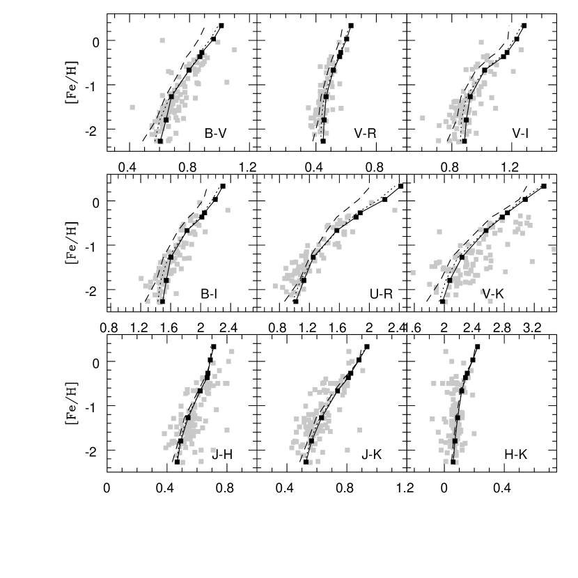
Figure 1: The Teramo-SPoT models compared to observational data. The models refer to three different ages: 5 Gyr (dashed lines), 11 Gyr (dotted lines) and 13 Gyr (solid lines, reference models). The gray dots mark Galactic GC data.

Figure 1 shows the MC relations from the SPoT models for several different colors. Data for the Galactic GCs are also shown. The optical colors and the [Fe/H] values for the Galactic GCs are taken from the Harris (1996) updated online catalog, while the near-IR photometric data are from Brocato et al. (1990) and Cohen et al. (2007). As seen in Fig. 1, the models provide a good match to the integrated properties of the Galactic GC system. The “wavy” behavior of the MC relations for the $(V{-}I)$, $(B{-}I)$, $(U{-}R)$, and $(B{-}V)$ colors is clearly evident. Furthermore, it is worth emphasizing the general nonlinearity of the MC relations for all the colors shown in the figure.

2.1 GC Simulations: SPoT models

We have developed a procedure to simulate a GC population with an arbitrary metallicity distribution and number of objects. Throughout this paper, however, we will consider the case of Gaussian metallicity distributions, and we simulate GC populations composed of 1000 objects. Armed with the MC relations of our reference models, the metallicity distribution of the GC system is randomly populated and projected into a color distribution. Finally, we use the KMM code (McLachlan & Basford, 1988; Ashman et al., 1994) to test whether the GC color distribution is best fit by a single or double Gaussian function.

In Figure 2 (left panel), we show the results of one of these simulations. Specifically, in this case we have simulated a metallicity distribution similar to the one adopted by YYL06, that is a Gaussian with peak at [Fe/H]$\,=-0.65$ dex and dispersion $\sigma_{[Fe/H]}=0.5$ dex. It is clearly recognized from the $(V{-}I)$ panel that the projected color distribution is bimodal. By running the KMM code, we find that, for this specific simulation, all the optical colors and the $(J{-}K)$ color distributions are significantly bimodal, while the optical to near-infrared colors, including $(I{-}H)$, have unimodal distributions.

As a check to these simulations, we have also made some numerical experiments adopting a bimodal metallicity distribution. In particular, Figure 2 (right panel) shows a simulation carried out adopting the bimodal metallicity distribution of the Galactic GC system, obtained using the prescriptions of Côté (1999). In the Figure also the observed metallicity and color distributions of Galactic GCs are shown. The histograms of the simulated GC population are shown with solid lines in the panels, while the histograms for the actual observed Galactic GCs are shown with dotted lines. To simulate observational scatter of the data, we have included a 10% Gaussian scatter in the colors. As can be seen from this comparison, there is generally a good match between the simulated and actual color histograms of the Galactic GC system.

Since our goal here is to identify the colors least affected by the projection bias, regardless of the underlying metallicity distribution, we have performed various tests assuming unimodal Gaussian distributions with peaks at [Fe/H]$\,=-1.65,-1.15,-0.65,-0.15$ dex and three values for the dispersion: $\sigma_{[Fe/H]}=0.25,0.5,0.75$ dex. For each of the twelve ([Fe/H], $\sigma_{[Fe/H]}$) pairs, we have simulated a GC system with a unimodal metallicity distribution and evaluated the colors of each GC according to the adopted MC relations. Afterwards, by using the KMM code, we estimate the likelihood, $P(bimodal)$, that the color distribution is better represented by two Gaussians than a single Gaussian, for various color choices. Values of $P(bimodal){\,\approx\,}1$ mean that the color distribution is likely bimodal; conversely, color distributions with $P(bimodal){\,\approx\,}0$ are likely unimodal. We have run the simulations both with and without including a 10% Gaussian scatter in the simulated colors.

Table 1 gives the results of these simulations. For each color index, the table lists the locations of the best-fitting blue and red peaks and the value of $P(bimodal)$ for each choice of mean metallicity and dispersion. The results are also shown graphically in the Figure 3, where solid dots mark the results for simulations without any color errors, and open circles mark results obtained with the random 10% color scatter. The different rows and columns refer to different mean [Fe/H] and $\sigma$ values, respectively, as labeled.

Two considerations emerge from inspection of Figure 3. First, according to the SPoT models, the projection effect that causes a unimodal metallicity distribution to be observed as a bimodal color distribution is not a unique characteristic of the HB-sensitive colors. It is, instead, present for most of the analyzed colors. For example, in the case of $(J{-}K)$, almost half of the numerical experiments carried out give bimodal color distributions [$P(bimodal)\sim 1.0$]. Thus the nonlinearity of the MC relation is not specific to just one or a few colors, such as the $(g-z)$ and $(V{-}I)$ colors discussed by YYL06. Although, as shown in Figure 1, different colors are affected differently by nonlinearity in the MC relation.

The second consideration that emerges from these simulations regards how the presence of color scatter (i.e. the photometric uncertainty) can affect the probability of obtaining a bimodal color distribution. The addition of color scatter can of course decrease the probability of bimodality by smoothing out the separation between the peaks. More surprisingly, it can also make bimodality appear more probable by removing sharp features from the color distributions, and thus significantly improving the goodness-of-fit of the double Gaussian model used by KMM.

It is interesting to note that the two extreme metallicities, [Fe/H]$\,=-1.65$ and $-$0.15 dex, result in strictly-unimodal, and generally-bimodal, color distributions, respectively (see also Yoon et al., 2006, their Fig. 3). Moreover, simulations with larger $\sigma$ values are in almost all cases more bimodal. Thus, for the combination ([Fe/H]$\,=-$0.15, $\sigma{\,=\,}0.75$), the color distributions are significantly bimodal for all simulated colors, but again this is an extreme case. The color distributions (as indicated by the peaks in Table 1) obtained from the most extreme simulations are not typical of those normally observed for extragalactic GC systems.

In order to refine our study, we now focus on those simulations best matching real GC systems. We have compared the color peaks from Table 1 with observed color peaks from literature. In particular, we have selected as “realistic” the simulations with:

• $(V-I)_{0,blue}\sim 0.95$ and $(V-I)_{0,red}\sim 1.15$, based on the Brodie & Strader (2006) compilation for bright (mainly E and S0) galaxies with $M_{B}\leq-18.5$ mag.

• $(B-I)_{0,blue}\sim 1.94$ and $(B-I)_{0,red}\sim 2.06$, derived from the Harris et al. (2006) sample of bright galaxies.

• $(I-H)_{0,blue}\sim 1.3$ and $(I-H)_{0,red}\sim 1.7$, from Kundu & Zepf (2007), based on M 87.

In order to avoid any bias towards bimodal distributions, we have also considered as realistic those unimodal color distributions whose peak is equal to the averaged blue and red peak colors reported above. By matching these criteria with the simulations, we have found that only the subset of simulations with [Fe/H]$\,=-$1.15, $-$0.65 and $\sigma_{[Fe/H]}=0.5,0.75$ provide realistic ranges for the color peaks. For example, the peaks for the $(V{-}I)$, $(B{-}I)$, and $(I{-}H)$ colors for the case of ([Fe/H]$\,=-$1.15, $\sigma_{[Fe/H]}=0.75$) are all in good agreement with the observational values listed above, even though most of these colors are found to have unimodal color distributions for this particular simulation.

By inspecting only the panels for the selected “realistic” simulations in Figure 3 (the panels labeled with an “S”), one can see that the colors $(B{-}V)$, $(V{-}I)$, and $(B{-}I)$ have, on average, an increased probability of being projected to a bimodal distribution, while colors such as $(I{-}K)$, $(V{-}H)$and $(V{-}K)$ have lower probabilities. Thus, if one wants to minimize the bias from the MC projection effect in real observations, i.e. if the contribution to bimodality due to a nonlinear MC relation is to be neglected, then the $(I{-}K)$, $(V{-}H)$, and $(V{-}K)$ colors are to be preferred.

Finally, we must emphasize that the above conclusions do not change if we adopt different ages. In fact, although there is some shift in color, the MC profiles are not strongly affected even when the $t=5$ Gyr models are considered (Figure 1). Since the projection effect is due to the shape of the MC relation (that is, to the changing derivative of the relation), and not to the absolute color values, this explains why the outcome of the simulations does not change significantly with age. In more detail, for the Raimondo et al. (2005) models at an age of $t=5$ Gyr, the “wavy” MC relation is mostly related to the appearance of the HB at metallicities [Fe/H]$\ \raise-2.0pt\hbox{\hbox to0.0pt{\hbox{$\sim$}\hss}\raise 5.0pt\hbox{$<$}\ }-0.4$ dex, while no HB is present at higher [Fe/H]. Finally, it is worth noting that the above results do not change substantially if the numerical experiments are carried out using a different number of simulated GCs.

2.2 Other SSP models

The results presented in the previous Section are based on a particular choice of the MC relations derived from the SPoT SSP models. In order to verify the robustness of those results, in this section we perform the same analysis discussed above, but with the MC relations derived from four other sets of SSP models. We consider the Maraston (2005), Anders & Fritze-v. Alvensleben (2003), Bruzual & Charlot (2003) and Lee et al. (2002) models (hereafter Mar05, And03, BC03, and Lee02, respectively).

We emphasize that, with the lone exception of the Lee02 models, the quoted models are computed with the primary aim of deriving the integrated photometric properties of stellar systems. This means that, in contrast to the SPoT models, they are not constrained to match as well with the specific features of observed CMDs. As a consequence, the detailed shape of the MC relation may not take into account the effect of stars in a particular evolutionary phase, which is a key point for a detailed modeling of the MC relations. Keeping in mind this warning, we perform for these models the same analysis discussed above for the SPoT models. For these simulations we again adopt a model age of 13 Gyr, except for the Lee02 models, which do not include this age, so we use their 14 Gyr models. The results of the simulations are presented in Figure 4, where we show only the results for the selected “realistic” simulations, although this choice does not substantially affect the our conclusions.

Inspecting the panels of Figure 4, we find some differences with the results based on the SPoT models. For example, the values of $P(bimodal)$ are low for the BC03 $(B{-}V)$, $(V{-}I)$, and $(B{-}I)$ colors distributions. This result for the BC03 models is not surprising, due to their lack of detailed HB morphology modeling, which is the main cause of the wavy MC relations for these colors. In contrast, the $(J{-}K)$ colors from the BC03 models are almost always bimodal, a result of some non-linearity in their MC relation unrelated to HB morphology. On the other hand, the Lee02 models, where nonlinear effects in the MC relation are stronger with respect to other models, generally predict higher $P(bimodal)$ values..

By making a cross-check of the results based on these sets of SSP models with the ones based on the SPoT models, we find that no one color is completely unaffected by MC projection bias. However, in almost all cases the $(V{-}H)$ and $(V{-}K)$ colors are predicted to be less affected by this bias. Thus, these mixed optical–IR colors should be preferred for GC studies, since, in normal galaxies, a bimodal distribution in these colors is more likely linked to an underlying bimodal metallicity distribution.

3 Conclusions

In this work we have performed a series of numerical experiments to simulate the properties of GC populations observed in different photometric colors. Our aim was to study how the nonlinear behavior of the MC relations affect a unimodal (Gaussian) metallicity distribution when it is projected into various optical and near-IR color distributions. By using the MC relations from the SPoT models, we have found that a unimodal metallicity distribution can be projected into a bimodal color distribution in almost any of the colors considered here, depending on the properties of the metallicity distribution, on the particular color index, and on the photometric uncertainty of the sample.

This result is due to the fact that all the MC relations are by and large nonlinear. To reduce the possibility of this bias in real data, and thus help ensure that an observed bimodal color distribution is due to a bimodal metallicity, one should choose a color whose MC relation is nearly linear. Since, for the grid of colors that we have considered here, there is no such “unbiased” color, the best colors to use are those that are most robust against this effect. Using the SPoT models, we have concluded that optical–to–near-IR colors are the best choices to disclose real bimodal metallicity distributions.

In order to assess model systematics and make more firm conclusions, we have also investigated several other sets of stellar population models. As a general result, the differences existing between model predictions do not allow us to pick any color index as safely unaffected by the metallicity projection bias. However, all models considered here, including the SPoT ones, predict that the bias effect is reduced for $(V{-}K)$, $(V{-}H)$, and similar colors. One other result of these simulations is that photometric uncertainties can affect, in surprising ways, the probability of obtaining a bimodal color distribution from the KMM algorithm. Thus, decreasing the statistical errors in real color data can help to avoid false detection of significant bimodality.

Further information on metallicity bimodality can of course come from the analysis of spectroscopic data for a significant number of GCs in galaxies with observed color bimodality. However, such observations are time consuming, and only feasible for relatively nearby objects. In addition, certain spectroscopic indices may themselves be affected by similar nonlinear relations with metallicity.

In conclusion, we confirm $(V{-}H)$ and $(V{-}K)$ as good colors to reveal (nearly) unbiased bimodal metallicity distributions in extragalactic GC systems. Future data on large GC samples in individual galaxies, including optical and near-IR photometry, as well as spectroscopy, coupled with further advances in stellar population modeling, should finally resolve this issue. Until that time, the interpretation of bimodal color distributions will remain, at least in part, ambiguous.

Figure 2: Left panel: The color histograms obtained from a unimodal (Gaussian) metallicity distribution with mean [Fe/H]$\,=-0.65$, $\sigma_{\rm[Fe/H]}=0.5$ (shown in the upper left panel). We find that all the optical and the $(J{-}K)$ color distributions are bimodal based on the KMM algorithm, while for the other colors a double Gaussian distribution does not significantly improve the fit to the data. Right panel: Simulation of a bimodal metallicity distribution (solid lines), chosen to match the Galactic GC distribution. The observed color histograms for the Galactic GCs are also shown with dotted lines (the observed metallicity distribution is shown in the upper left panel with dotted histogram). The parameters used for the simulated distribution are [Fe/H]${}_{low}=-1.59$, $\sigma_{[Fe/H],low}=0.30$ dex, and [Fe/H]${}_{high}=-0.55$, $\sigma_{[Fe/H],high}=0.27$ dex, with a photometric uncertainty of 10%, and the N_low to N_high ratio is 2.

Figure 3: The probability $P(bimodal)$ of having a bimodal color distribution starting from a unimodal Gaussian metallicity distribution is shown for different color indices and various metallicity distributions. Left/middle/right panels refer to simulations with $\sigma=0.25,0.5,0.75$ dex, respectively (see upper labels). Different rows refer to different mean metallicities, as labeled. High (low) values of $P(bimodal)$ mean that the color distribution is significantly bimodal (unimodal). Filled dots mark numerical experiments without any color scatter, and open circles show simulations including a 10% color scatter. Although all the simulated metallicity distributions are unimodal, about 45% of these color distributions are found to be bimodal. The four panels with the “S” label refer to the simulations that best match with observed GC color ranges.

Figure 4: Same as Figure 3, but for MC relations taken from other sets of SSP models (labeled at the top of each set of panels). Only the results for the simulations matching with observed GC colors are shown.

Table 1: Simulations of GC population

[Fe/H], $\sigma$	$(B-V)_{0}$	$(V-I)_{0}$	$(B-I)_{0}$	$(I-H)_{0}$	$(I-K)_{0}$	$(J-K)_{0}$	$(V-H)_{0}$	$(V-K)_{0}$	$(U-R)_{0}$	$(B-H)_{0}$	$(B-K)_{0}$
(dex)	blue red Pb	blue red Pb	blue red Pb	blue red Pb	blue red Pb	blue red Pb	blue red Pb	blue red Pb	blue red Pb	blue red Pb	blue red Pb
	GC simulations without color scatter
$-$1.65 0.25	0.66 0.66 0.0	0.91 0.91 0.0	1.57 1.57 0.0	1.15 1.16 0.0	1.22 1.24 0.0	0.59 0.59 0.0	2.05 2.07 0.0	2.13 2.31 0.2	1.17 1.19 0.0	2.71 2.94 0.2	2.79 3.02 0.2
$-$1.15 0.25	0.72 0.72 0.0	0.95 0.96 0.0	1.65 1.79 0.2	1.25 1.35 1.0	1.34 1.46 1.0	0.66 0.67 0.0	2.19 2.36 1.0	2.29 2.47 1.0	1.32 1.51 0.4	2.90 3.13 1.0	3.00 3.24 1.0
$-$0.65 0.25	0.81 0.82 0.0	1.02 1.14 1.0	1.80 2.00 1.0	1.42 1.44 0.0	1.55 1.56 0.0	0.75 0.76 0.0	2.43 2.63 1.0	2.56 2.79 1.0	1.58 1.85 1.0	3.22 3.49 1.0	3.35 3.65 1.0
$-$0.15 0.25	0.92 0.93 0.0	1.08 1.21 0.2	1.95 2.14 0.2	1.56 1.74 0.4	1.72 1.93 1.0	0.85 0.86 0.0	2.74 2.94 0.6	2.90 3.12 1.0	1.88 2.21 1.0	3.62 3.87 0.9	3.77 4.07 1.0
$-$1.65 0.5	0.67 0.67 0.0	0.91 0.92 0.0	1.56 1.80 0.2	1.12 1.32 0.4	1.21 1.43 0.4	0.58 0.61 0.0	2.04 2.37 0.2	2.12 2.49 0.2	1.16 1.53 0.2	2.69 3.15 0.2	2.77 3.26 0.3
$-$1.15 0.5	0.70 0.84 0.4	0.95 1.14 0.4	1.65 2.00 0.4	1.23 1.42 1.0	1.37 1.63 0.2	0.64 0.78 0.4	2.20 2.60 0.4	2.30 2.76 0.4	1.33 1.85 0.4	2.90 3.44 0.4	3.00 3.60 0.4
$-$0.65 0.5	0.76 0.91 1.0	0.99 1.19 1.0	1.75 2.10 1.0	1.41 1.76 0.2	1.53 1.94 0.2	0.70 0.83 1.0	2.41 2.84 0.4	2.53 3.04 0.4	1.54 2.14 1.0	3.18 3.75 1.0	3.30 3.95 1.0
$-$0.15 0.5	0.83 0.97 1.0	1.03 1.24 1.0	1.86 2.20 1.0	1.54 1.91 1.0	1.69 2.13 1.0	0.77 0.89 1.0	2.68 3.12 1.0	2.82 3.33 1.0	1.75 2.34 1.0	3.52 4.06 1.0	3.66 4.28 1.0
$-$1.65 0.75	0.65 0.85 0.4	0.91 1.16 0.2	1.57 2.02 0.2	1.14 1.48 0.0	1.22 1.70 0.0	0.57 0.77 0.3	2.04 2.63 0.2	2.12 2.80 0.2	1.17 1.90 0.2	2.69 3.48 0.3	2.77 3.64 0.3
$-$1.15 0.75	0.70 0.91 1.0	0.94 1.19 1.0	1.64 2.11 1.0	1.27 1.79 0.0	1.37 1.97 0.2	0.63 0.82 1.0	2.19 2.84 0.4	2.29 3.05 0.4	1.32 2.14 0.2	2.89 3.74 0.4	2.99 3.95 0.4
$-$0.65 0.75	0.75 0.96 1.0	0.97 1.23 1.0	1.71 2.19 1.0	1.39 1.93 0.4	1.51 2.15 0.4	0.68 0.87 1.0	2.39 3.09 0.6	2.50 3.31 0.6	1.49 2.34 1.0	3.14 4.03 1.0	3.25 4.26 1.0
$-$0.15 0.75	0.80 1.01 1.0	1.01 1.27 1.0	1.81 2.28 1.0	1.53 2.08 0.6	1.67 2.33 1.0	0.75 0.93 0.9	2.63 3.33 1.0	2.77 3.58 1.0	1.68 2.51 1.0	3.45 4.32 1.0	3.59 4.57 1.0
	GC simulations including 10% color scatter
$-$1.65 0.25	0.66 0.66 0.0	0.91 0.91 0.0	1.56 1.58 0.0	1.13 1.17 0.0	1.22 1.25 0.0	0.59 0.60 0.0	2.05 2.07 0.0	2.13 2.29 0.2	1.16 1.20 0.0	2.70 2.74 0.0	2.79 3.01 0.0
$-$1.15 0.25	0.72 0.73 0.0	0.95 0.96 0.0	1.66 1.69 0.0	1.24 1.35 0.9	1.34 1.47 1.0	0.66 0.67 0.0	2.20 2.36 1.0	2.29 2.48 1.0	1.31 1.50 0.6	2.89 3.12 1.0	2.99 3.23 1.0
$-$0.65 0.25	0.81 0.82 0.0	1.02 1.14 1.0	1.80 1.99 1.0	1.42 1.44 0.0	1.55 1.56 0.0	0.74 0.77 0.1	2.43 2.63 1.0	2.56 2.80 1.0	1.58 1.85 1.0	3.21 3.48 1.0	3.34 3.64 1.0
$-$0.15 0.25	0.87 0.96 1.0	1.08 1.21 1.0	1.97 2.16 0.4	1.56 1.75 0.4	1.72 1.94 1.0	0.84 0.86 0.0	2.74 2.94 1.0	2.89 3.14 0.9	1.87 2.21 1.0	3.60 3.87 0.9	3.76 4.07 1.0
$-$1.65 0.5	0.66 0.78 0.2	0.91 1.06 0.0	1.57 1.81 0.2	1.11 1.26 0.9	1.21 1.45 0.2	0.57 0.68 0.4	2.04 2.37 0.2	2.12 2.49 0.3	1.17 1.54 0.2	2.70 3.15 0.3	2.78 3.27 0.3
$-$1.15 0.5	0.70 0.85 0.4	0.95 1.14 0.4	1.66 2.00 0.4	1.25 1.43 0.9	1.38 1.70 0.0	0.63 0.77 1.0	2.20 2.59 0.4	2.30 2.76 0.4	1.33 1.85 0.4	2.90 3.44 0.4	3.00 3.60 0.4
$-$0.65 0.5	0.76 0.91 1.0	0.99 1.19 1.0	1.75 2.09 1.0	1.41 1.78 0.2	1.53 1.96 0.2	0.70 0.84 1.0	2.41 2.84 0.6	2.53 3.05 0.4	1.54 2.14 1.0	3.18 3.74 1.0	3.30 3.96 1.0
$-$0.15 0.5	0.83 0.98 1.0	1.03 1.23 1.0	1.86 2.21 1.0	1.54 1.91 0.6	1.69 2.14 1.0	0.78 0.90 0.8	2.68 3.11 1.0	2.82 3.34 1.0	1.75 2.34 1.0	3.51 4.05 1.0	3.67 4.29 1.0
$-$1.65 0.75	0.66 0.86 0.3	0.91 1.15 0.3	1.57 2.01 0.3	1.15 1.56 0.0	1.23 1.76 0.0	0.57 0.76 0.4	2.04 2.63 0.2	2.12 2.80 0.2	1.18 1.91 0.2	2.69 3.48 0.3	2.78 3.65 0.3
$-$1.15 0.75	0.70 0.92 0.6	0.94 1.20 0.6	1.64 2.11 1.0	1.27 1.82 0.0	1.37 2.00 0.2	0.62 0.82 1.0	2.19 2.84 0.4	2.29 3.05 0.4	1.32 2.14 0.4	2.89 3.75 0.4	3.00 3.95 0.4
$-$0.65 0.75	0.75 0.96 1.0	0.97 1.23 1.0	1.72 2.19 1.0	1.40 1.94 0.3	1.51 2.15 0.4	0.68 0.88 1.0	2.38 3.09 0.6	2.50 3.31 0.6	1.49 2.34 1.0	3.14 4.03 1.0	3.26 4.27 1.0
$-$0.15 0.75	0.80 1.01 1.0	1.01 1.27 1.0	1.80 2.28 1.0	1.52 2.08 1.0	1.67 2.33 1.0	0.76 0.94 0.9	2.62 3.33 1.0	2.77 3.59 1.0	1.68 2.51 1.0	3.45 4.31 1.0	3.60 4.57 1.0

References

- Anders & Fritze-v. Alvensleben (2003) Anders, P., & Fritze-v. Alvensleben, U. 2003, A&A, 401, 1063 (And03)
- Ashman et al. (1994) Ashman, K. M., Bird, C. M., & Zepf, S. E. 1994, AJ, 108, 2348
- Brocato et al. (1990) Brocato, E., Caputo, F., di Giorgio, A. M., Santolamazza, P., & Richichi, A. 1990, Memorie della Societa Astronomica Italiana, 61, 137
- Brocato et al. (2000) Brocato, E., Castellani, V., Poli, F. M., & Raimondo, G. 2000, A&AS, 146, 91
- Brodie & Strader (2006) Brodie, J. P., & Strader, J. 2006, ARA&A, 44, 193
- Bruzual & Charlot (2003) Bruzual, G., & Charlot, S. 2003, MNRAS, 344, 1000 (BC03)
- Cantiello et al. (2005) Cantiello, M., Blakeslee, J. P., Raimondo, G., Mei, S., Brocato, E., & Capaccioli, M. 2005, ApJ, 634, 239
- Cantiello et al. (2007) Cantiello, M., Raimondo, G., Blakeslee, J. P., Brocato, E., & Capaccioli, M. 2007, ApJ, 662, 940
- Cohen et al. (2007) Cohen, J. G., Hsieh, S., Metchev, S., Djorgovski, S. G., & Malkan, M. 2007, AJ, 133, 99
- Côté (1999) Côté, P. 1999, AJ, 118, 406
- Harris (1996) Harris, W. E. 1996, AJ, 112, 1487
- Harris et al. (2006) Harris, W. E., Whitmore, B. C., Karakla, D., Okoń, W., Baum, W. A., Hanes, D. A., & Kavelaars, J. J. 2006, ApJ, 636, 90
- Kundu & Zepf (2007) Kundu, A., & Zepf, S. E. 2007, ApJ, 660, L109
- Lee et al. (2002) Lee, H.-c., Lee, Y.-W., & Gibson, B. K. 2002, AJ, 124, 2664 (Lee02)
- Maraston (2005) Maraston, C. 2005, MNRAS, 362, 799 (Mar05)
- McLachlan & Basford (1988) McLachlan, G. J., & Basford, K. E. 1988, Mixture models. Inference and applications to clustering (Statistics: Textbooks and Monographs, New York: Dekker, 1988)
- Peng et al. (2006) Peng, E. W. et al. 2006, ApJ, 639, 95
- Pietrinferni et al. (2004) Pietrinferni, A., Cassisi, S., Salaris, M., & Castelli, F. 2004, ApJ, 612, 168
- Raimondo et al. (2005) Raimondo, G., Brocato, E., Cantiello, M., & Capaccioli, M. 2005, AJ, 130, 2625 (SPoT)
- Reimers (1975) Reimers, D. 1975, Memoires of the Societe Royale des Sciences de Liege, 8, 369
- Richtler (2003) Richtler, T. 2003, in LNP Vol. 635: Stellar Candles for the Extragalactic Distance Scale, ed. D. Alloin & W. Gieren, 281–305
- Richtler (2006) Richtler, T. 2006, Bulletin of the Astronomical Society of India, 34, 83
- Scalo (1998) Scalo, J. 1998, in Astronomical Society of the Pacific Conference Series, Vol. 142, The Stellar Initial Mass Function (38th Herstmonceux Conference), ed. G. Gilmore & D. Howell, 201–+
- Wagenhuber & Groenewegen (1998) Wagenhuber, J., & Groenewegen, M. A. T. 1998, A&A, 340, 183
- West et al. (2004) West, M. J., Côté, P., Marzke, R. O., & Jordán, A. 2004, Nature, 427, 31
- Westera et al. (2002) Westera, P., Lejeune, T., Buser, R., Cuisinier, F., & Bruzual, G. 2002, A&A, 381, 524
- Yoon et al. (2006) Yoon, S.-J., Yi, S. K., & Lee, Y.-W. 2006, Science, 311, 1129 (YYL06)