A Synthetical Weights’ Dynamic Mechanism for Weighted Networks

Abstract

We propose a synthetical weights’ dynamic mechanism for weighted networks which takes into account the influences of strengths of nodes, weights of links and incoming new vertices. Strength/Weight preferential strategies are used in these weights’ dynamic mechanisms, which depict the evolving strategies of many real-world networks. We give insight analysis to the synthetical weights’ dynamic mechanism and study how individual weights’ dynamic strategies interact and cooperate with each other in the networks’ evolving process. Power-law distributions of strength, degree and weight, nontrivial strength-degree correlation, clustering coefficients and assortativeness are found in the model with tunable parameters representing each model. Several homogenous functionalities of these independent weights’ dynamic strategy are generalized and their synergy are studied.

1 Introduction

Complex networks [1, 2, 3, 4, 5] depict a great many real-world networks like the scientific collaboration networks (SCN) [6, 7, 8, 9], World Wide Web (WWW) [10], world-wide airport networks (WAN) [11, 12] and so on. Simple binary networks [1, 2, 3] are used to depict the topological aspects of these real-world networks. Degree distribution and degree related clustering coefficients can be analyzed from the model. Typically, Barabási and Albert proposed a linear preferential attachment model on which most other binary models are based on (BA model[13]). However, real-world networks often contains far more information than that binary networks can express, since relations in the networks are not necessarily binary. Therefore links with weights are introduced to emphasize the importance of heterogenous relations between nodes in networks. Barrat, Barthélemy and Vespignani first build a model for weighted networks based on preferential attachment mechanism (BBV model [14, 15]). Since then various models have been derived to mimic diverse real-world networks [4, 5, 16, 17, 18, 19, 20, 21, 22], all of which emphasize a different kind of weights’ dynamic mechanism.

The flourishing research on various weights’ dynamics mechanisms roots in the the heterogenous behaviors of real-life networks. Current research has already covered most part of typical behaviors of weights’ dynamics. However, the interaction and operations of these scattered weights’ dynamics are poorly studied and their underlying homogeneity are still not know. In our paper, we generalize weights’ dynamics with monotonous weights’ growth and focus on interactions and cooperations among them.

With a close scrutiny into prevailing weights’ dynamic models depicting real-world networks we find that there are three main sources of weights’ increment dynamics: the variation of traffic caused by introducing of new nodes [4, 5, 16, 17, 18, 19], the increment of links’ weights based on links’ weights themselves [23], and the increment of weights based on strength of two ends of the link [20, 21, 22]. Most weights’ increment dynamics can be grouped into these three sources. Many works have done to empirically validate the classification, among them Newman gives the most comprehensive and convincing experiments [24]. In this paper we will give numerical and analytical study to the synthetical weights’ dynamic model which comprises the three above-mentioned mechanisms, and reveal the scale-free characteristics and nontrivial clustering coefficients and assortativeness of the model.

Our paper is organized as follows. In Sec. $2$ we define basic definitions and terms to represent the weighted network and gives a brief review of related works done. In Sec. $3$ we depict our model and give clear definition of three weights’ dynamic mechanisms. In Sec. $4$ we analytically calculate the mathematical expression for probability distributions of strength and weight, degree-strength correlations and related attributes. In Sec. $5$ we preform simulations to mimic the proposed mechanisms and analyze the experiment results in detail. In Sec. $6$ we give a conclusion to the paper.

2 Definitions

Weighted networks can be represented by a adjacent matrix $W$ where $w_{ij}$ defines the weight of link between vertices $i$ and $j$. $w_{ij}=0$ indicates that there is no link between vertices $i$ and $j$. Therefore topological and weighted information can both be revealed from $W$. Matrix $W$ is symmetrical therefore $w_{ij}=w_{ji}$. Degree $k_{i}$ defines the number of vertices vertex $i$ is linked with, and strength $s_{i}$ defines the total weights of links that ends in the particular vertex $i$. $s_{i}$ can be written as $s_{i}=\sum_{j}w_{ij}$, and $k_{i}$ can be written as $k_{i}=\sum_{j}sgn(w_{ij})$, where $sgn()$ is the signum function. $P(s)$, $P(k)$, $P(w)$ defines the probability distribution of strength, degree and weight. Previous studies have revealed that in many weighted networks, $P(s)$, as well as $P(k)$ and $P(w)$, displays a power-law distribution as $P(s)=s^{-\gamma_{s}}$, $P(k)=k^{-\gamma_{k}}$ and $P(w)=w^{-\gamma_{w}}$. There is also a power-law correlation between $s$ and $k$ that $s=k^{\alpha}$. Clustering coefficients and assortativeness of weighted network is also studied and the details will be discussed later.

3 The Model

The model proposed in this paper starts from an initial configuration of $N_{0}$ vertices fully connected by links with weight $w_{0}=1$ ($N_{0}$-clique). At each time step, the network evolves under two coupled mechanisms: topological growth and weights’ dynamics. Weights’ dynamics are discussed in detail in this paper, where all three sources of weights’ dynamics are taken into account.

3.1 Topological Growth

At each time step, a new vertex $n$ is introduced into the network and connected to $p$ existing vertices $i$. Vertices are chosen according to the strength preferential probability

$$\Pi_{n\rightarrow i}=\frac{s_{i}}{\sum_{j}s_{j}}\,,$$ (1)

and the weight of this new link is set to $w_{0}=1$.

3.2 Weights’ Dynamics

There are three sources of weights’ dynamics: the local increment of weights triggered by the introduction of the new vertex, the self-increment of weights based on the weight of each link, and the mutual selection dynamics focusing on creation and reinforcement of links between existing vertices based on their strengths. These three weights’ dynamics mechanisms interact and cooperate during the evolution of the network. There are several suggestive independent works for these three sources weights’ dynamics: Barrat, Barthélemy, Vespignani first suggest the local rearrangement model considering the impact of incoming vertices. Dorogovtsev, Mendes’s work Wen-Xu Wang’s works suggest the mutual selection model which well depict the second source. ********’s work initializes the idea of weights’ self-increment although the idea is not comprehensively studied yet. There are lots of works done that empirically proving the validity of the three sources. Newman in his work by empirically studying the scientific collaboration network suggests that two scientists would have better chance to enforce their collaboration if they already have a lot of works together, and scientists are more likely to develop new collaborative relationships if they already have relatively large numbers of collaborators [24]. Collaborative relationships of scientists and their collaborators are analogous to weights and degree in a network. Degree can be generalized to strength if we take into account the amount of collaborations between each pairs of collaborators in stead of a binary expression.

The introduction of new vertex brings variation in traffic across the network. For simplicity, we restrict the variation to the neighborhood of vertex $i$ which has just been chosen to link with the new vertex. An overall increment of $\delta$ is introduction at each time step. The increment is distributed among the neighborhood of $\Gamma(i)$ according to weight preferential mechanism:

$$w_{ij}\rightarrow w_{ij}+\delta\frac{w_{ij}}{s_{i}}\,.$$ (2)

The strengths of $i$ and all $j\in\Gamma(i)$ are also increased as a result of the increment of weights in the neighborhood of $i$. Considering the probability of vertices $i$ been chosen, the increment of $w_{ij}$ can be rewritten as

$$\Delta w_{ij} =p\frac{s_{i}}{\sum_{k}s_{k}}\delta\frac{w_{ij}}{s_{i}}+p\frac{s_{j}}{\sum_{k}s_{k}}\delta\frac{w_{ij}}{s_{j}}$$

$$=2p\delta\frac{w_{ij}}{\sum_{k}s_{k}}\,.$$ (3)

At each time step, $n$ existing links are chosen to increase according to the weight preferential probability:

$$w_{ij}\rightarrow w_{ij}+n\frac{w_{ij}}{\sum_{k,l}w_{kl}}$$ (4)

Each chosen link is increased by $w_{0}=1$. The links with larger weights always have more chance to reinforcement.

At each time step, each existing vertex $i$ selects $m$ vertices according to the strength preferential mechanism:

$$\Pi_{i\rightarrow j}=m\frac{s_{j}}{\sum_{k}s_{k}-s_{i}}\,.$$ (5)

There would be a alteration in links between $i$ and $j$ if and only if $i$ and $j$ have mutually selected each other. The probability that the linking condition between $i$ and $j$ changes can be defined to be:

$$\Pi_{i,j} =m\frac{s_{j}}{\sum_{k}s_{k}-s_{i}}m\frac{s_{i}}{\sum_{k}s_{k}-s_{j}}$$

$$=m^{2}\frac{s_{i}s_{j}}{(\sum_{k}s_{k}-s_{i})(\sum_{k}s_{k}-s_{j})}$$

$$\approx m^{2}\frac{s_{i}s_{j}}{(\sum_{k}s_{k})^{2}}\,.$$ (6)

If there is not a link between $i$ and $j$, a new link with assigned weight $w_{0}=1$ will be added. If there is already a link between $i$ and $j$, the link will be increased by $w_{0}=1$.

These three weights’ dynamics mechanisms interact and cooperate during the the process of network development. Synthesize all the these three mechanisms, the increment of weights can be represented to be

$$w_{ij}\rightarrow w_{ij}+2p\delta\frac{w_{ij}}{\sum_{k}s_{k}}+n\frac{w_{ij}}{\sum_{k,l}w_{kl}}+m^{2}\frac{s_{i}s_{j}}{(\sum_{k}s_{k})^{2}}\,.$$ (7)

Noticing the fact that $\sum_{k,l}w_{kl}=\frac{1}{2}\sum_{k}s_{k}$, we can rewrite the above equation as

$$w_{ij}\rightarrow w_{ij}+(2p\delta+2n)\frac{w_{ij}}{\sum_{k}s_{k}}+m^{2}\frac{s_{i}s_{j}}{(\sum_{k}s_{k})^{2}}\,.$$ (8)

4 Evolution and Distribution of Degree, Strength and Weight

Using the continuous approximation, we can assume that $s$, $k$, $w$, $t$ are all continuous. Therefore we get

$$\frac{dw_{ij}}{dt}=(2p\delta+2n)\frac{w_{ij}}{\sum_{k}s_{k}}+m^{2}\frac{s_{i}s_{j}}{(\sum_{k}s_{k})^{2}}\,.$$ (9)

There are two sources contributing the increment of strength $s_{i}$, one is the weights’ dynamic and the other is linking with the new added node. Therefore the increment of $s_{i}$ can be written as

$$\frac{ds_{i}}{dt} =\sum_{j}\frac{dw_{ij}}{dt}+p\frac{s_{i}}{\sum_{k}s_{k}}$$

$$=(m^{2}+2p\delta+2n+p)\frac{s_{i}}{\sum_{k}s_{k}}\,.$$ (10)

The sum of strength of all nodes $\sum_{k}s_{k}$ at time $t$ can be calculated as

$$\sum_{k}s_{k}(t) =\sum_{1}^{t}s_{i}$$

$$=\int_{0}^{t}\sum_{k}\frac{ds_{k}}{dt}+pt$$

$$=(m^{2}+2p\delta+2n+2p)t\,,$$ (11)

and using this equation we can rewrite Eq. (4) as

$$\frac{ds_{i}}{dt}=\frac{m^{2}+2p\delta+2n+p}{m^{2}+2p\delta+2n+2p}\frac{s_{i}}{t}\,.$$ (12)

With the initial condition $s_{i}(t=i)=1$, we can integrate the above equation to obtain

$$s_{i}(t)=\left(\frac{t}{i}\right)^{\frac{m^{2}+2p\delta+2n+p}{m^{2}+2p\delta+2n+2p}}$$ (13)

From the equation we can see that three parameters $m$, $\delta$ and $n$ cooperatively and interactively govern the growing speed of strength $s_{i}$. Is is really amazing to find out that all three sources of weights’ dynamics influence the growing speed of strength in similar ways. The simulation of evolution of $s_{i}$ is given in Fig. 1. We see how $m$, $\delta$, $n$, $p$ contribute to the evolution of $s_{i}$ independently by fixing three other parameters. We also show how these four parameters interact by varying them the same time as indicated by the above equation. We see $s_{i}$ display a power-law distribution as $t$ evolves, and variable $m$ contribute larger alteration in $s_{i}$ with relatively small amount of increment.

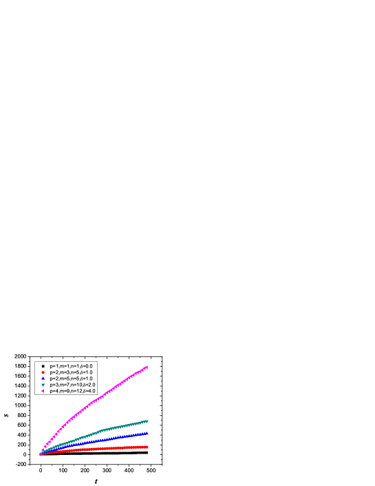
Figure 1: Evolution of degree $s_{i}$ with time for vertex $i=1$, the time span is from 1 to 5000 and the result is average of 10 individual experiments. Various values for $p$, $m$, $n$, $\delta$ are chosen to display the interplay of different parameters.

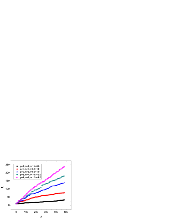
Figure 2: Evolution of degree $k_{i}$ with time for vertex $i=1$, the time span is from 1 to 5000 and the result is average of 10 individual experiments. Various values for $p$, $m$, $n$, $\delta$ are chosen to display the interplay of different parameters.

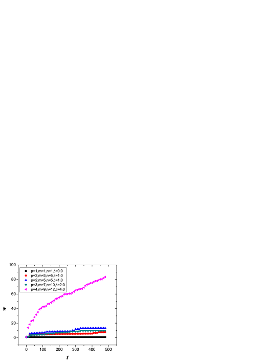
Figure 3: Evolution of degree $w_{i}$ with time for vertex $i=1$ and $j=2$, the time span is from 1 to 5000 and the result is average of 10 individual experiments. Various values for $p$, $m$, $n$, $\delta$ are chosen to display the interplay of different parameters.

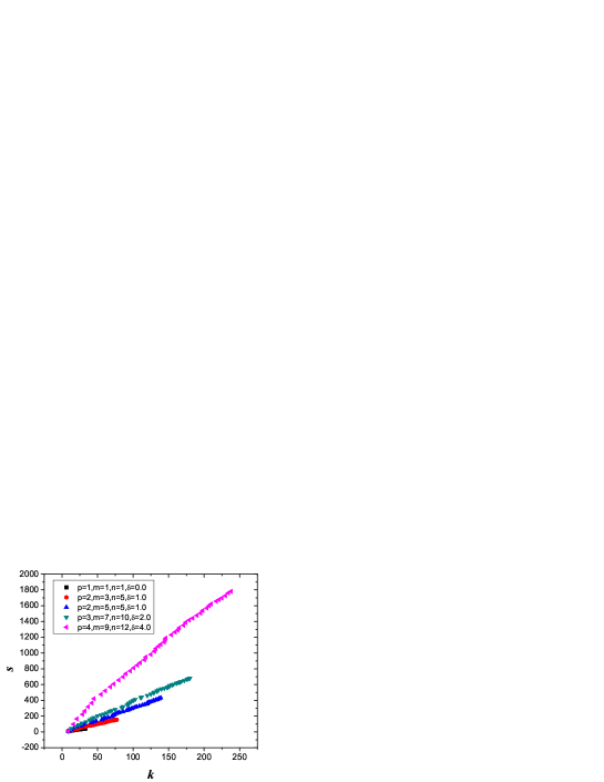
Figure 4: Nontrivial correlation between degree $k$ and strength $s$, the size of the network is 5000 and the result is average of 10 individual experiments. Various values for $p$, $m$, $n$, $\delta$ are chosen to display the interplay of different parameters.

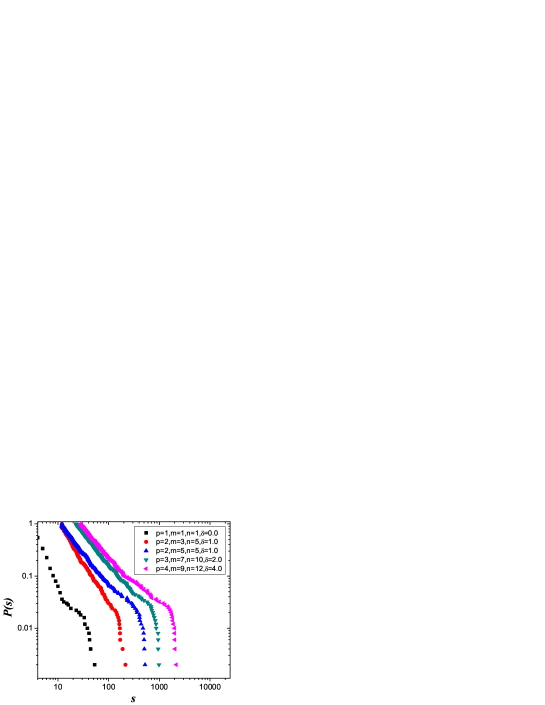
Figure 5: Power-law probability distribution of strength $s$, the size of the network is 5000 and the result is average of 10 individual experiments. Various values for $p$, $m$, $n$, $\delta$ are chosen to display the interplay of different parameters.

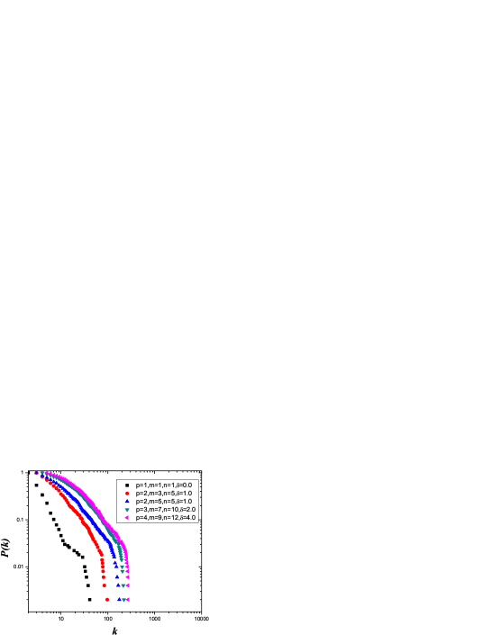
Figure 6: Power-law probability distribution of degree $k$, the size of the network is 5000 and the result is average of 10 individual experiments. Various values for $p$, $m$, $n$, $\delta$ are chosen to display the interplay of different parameters.

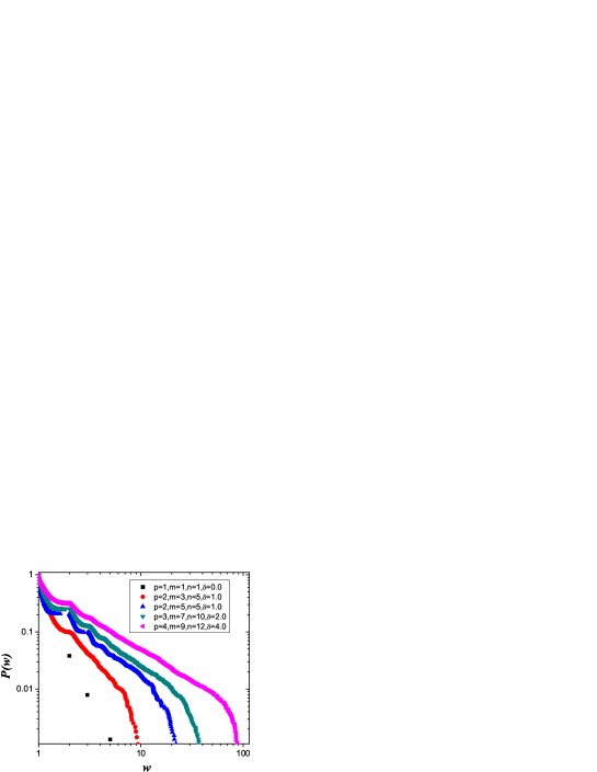
Figure 7: Power-law probability distribution of weight $w$, the size of the network is 5000 and the result is average of 10 individual experiments. Various values for $p$, $m$, $n$, $\delta$ are chosen to display the interplay of different parameters.

The knowledge of the time evolution of the various quantities allows us to compute their statistical properties. The incoming time $t_{i}$ of each vertex $i$ is uniformly distributed in $[0,t]$ and the strength probability distribution can be written as

$$P(s,t)=\frac{1}{t+N_{0}}\int_{0}^{t}\delta(s-s_{i}(t))dt_{i}\,,$$ (14)

where $\delta(x)$ is the Dirac delta function. Using Eq. (13) we can get in the infinite size limit $t\rightarrow\infty$ the distribution $P(s)\sim s^{-\gamma_{s}}$ with

$$\gamma_{s}=2+\frac{p}{m^{2}+2p\delta+2n+p}\,.$$ (15)

The degree probability distribution $P(k)\sim k^{-\gamma_{k}}$ can be obtained by combining $s\sim k^{\beta}$ with Eq. (13). From the equation of the conservation of probability

$$\int_{0}^{\infty}P(k)dk=\int_{0}^{\infty}P(s)ds$$ (16)

we can get

$$P(k)\sim P(s)\frac{ds}{dk}\sim s^{-\gamma_{s}}\beta k^{\beta-1}\sim\beta k^{-[\beta(\gamma_{s}-1)+1]}\,,.$$ (17)

Therefore we get $\gamma_{k}=\beta(\gamma_{s}-1)+1$ in $P(k)\sim k^{-\gamma_{k}}$. The simulations of $k_{i}$ and $P(k)$ are given in Fig. 2 and Fig.Fig. 6 with resemble the figures for $s_{i}$ and $k_{i}$. The power-law correlation between $s$ and $k$ is reveal by Fig. 4, where we fix $m=p=1$ and tune $\delta$ and $n$ as we need. .

The evolution and distribution of weight can be calculated similarly as we deal with strength. Combine Eq. (9), Eq. (4) ,Eq. (13), and define $a=m^{2}+2p\delta+2n+2p$, we get

$$\frac{dw_{ij}}{dt}=\frac{2p\delta+2n}{a}\frac{w_{ij}}{t}+\frac{m^{2}}{a^{2}}\left(\frac{1}{ij}\right)^{1-\frac{1}{a}}t^{-\frac{2}{a}}$$ (18)

we can integrate the above equation and get

$$w_{ij}\sim t^{\frac{m^{2}+2p\delta+2n}{m^{2}+2p\delta+2n+2p}}$$ (19)

for large $t$. Therefore $P(w)$ can be represented as $P(w)=w^{-\gamma_{w}}$ with $\gamma_{w}=2+\frac{2p}{m^{2}+2\delta+2n}$. The simulations of $w_{ij}$ and $P(w)$ are given representatives in Fig. 3 and Fig. 7.

5 Clustering Coefficients and Assortativeness

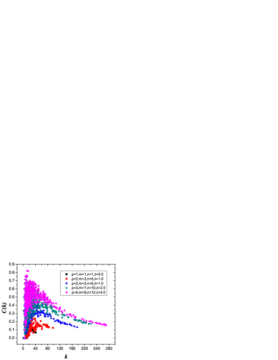
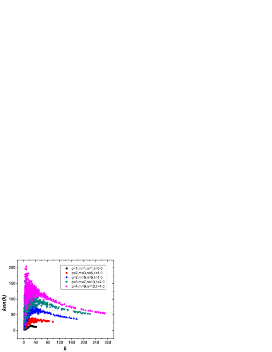
Figure 8: (a) Clustering coefficients for different degree $k$. (b) Average nearest-neighbor degree for different degree $k$. The size of the network is 5000 and the result is average of 10 individual experiments. Various values for $p$, $m$, $n$, $\delta$ are chosen to display the interplay of different parameters.

Clustering coefficients depict connectivity among neighborhood of given vertices. The local clustering coefficient $c_{i}$ for specific vertex $i$ is defined to be $c_{i}=\frac{1}{C_{k_{i}}^{2}}\sum_{j<k}sgn(w_{ij}w_{jk}w_{ik})$, which denotes the percentage of number of triangles in the neighborhood of $i$ to the number of potential triangles there. $c_{i}$ reveals how close vertices in the neighborhood of $i$ are related. The average $c_{i}$ of all vertices is denoted as $C$, and the average of $c_{i}$ for vertices with degree $k$ is denoted as $C(k)$. Average degree of nearest neighbor $knn,i$ for vertex $i$ is also studied, as well as $knn(k)$ for the average of $knn,i$ of vertices with degree of $k$. $knn$ reveals the assortativeness of a network.

We perform numerical experiment the simulate the growth of network and analyze the clustering coefficient and assortativeness under the synthetical weights’ dynamic mechanism. In Fig. 8(a) we show how clustering coefficients vary with tunable variables. The scale-free attributes $C$ measures the overall density of triangles in the network. We can see that $C$ is consistent with the network size $N$ while varying positively when those tunable variables change. The evolution of $knn$ is show in Fig. 8(b) which suggest the tunable assortativeness of the network.

6 Conclusion

In summary, we propose a new model for weighted networks which synthesizes three sources of weights’ dynamic: local weights’ rearrangement raised by introduction of new vertex; self-increment of weights according to weights’ preferential strategy; weights’ creation and reinforcement proportional to strengths of both ends of nodes. Three sources independently contribute to the evolution and in the mean time also cooperatively interact. The homogenous behaviors that these weights’ dynamics display suggest there may be some common underlying mechanisms that are not yet well understood. This model would be a good start for a synthetical and general understanding of weights’ dynamic and hopefully our work would be helpful for the future study.

References

- [1] R. Albert and A.-L. Barabási, Rev. Mod. Phys. 74, 47 (2002).
- [2] S. N. Dorogvtsev and J.F.F. Mendes, Adv. Phys. 51, 1079 (2002).
- [3] M. E. J. Newman, SIAM Review 45, 167 (2003).
- [4] S Boccaletti, V Latora, Y Moreno, M. Chavezf, and D.-U. Hwanga, Physics Report 424, 175 (2006).
- [5] K. Borner, S. Sanyal and A. Vespignani Ann. Rev. Infor. Sci. Tech. 41, 537 (2007).
- [6] M. E. J. Newman, Proc. Natl. Acad. Sci. U.S.A. 98 (2001) 404.
- [7] M. E. J. Newman, Phys. Rev. E 64, 016132 (2001).
- [8] A.-L. Barabási, H. Jeong, Z. Néda. E. Ravasz, A. Schubert, and T. Vicsek, Physica A 311, 590 (2002).
- [9] M Li, J Wu, D Wang, T Zhou, Z Di, Y Fan, Physica A 375, 355 (2007).
- [10] R. Albert, H. Jeong and A.-L. Barabási, Nature 401 (1999) 130.
- [11] A. Barrat, M. Barthélemy, R. Pastor-Satorras, and A. Vespignani, Proc. Natl. Acad. Sci. U.S.A. 101, 3747 (2004).
- [12] W. Li, and X. Cai, Phys. Rev. E 69, 046106 (2004).
- [13] A.-L. Barabási and R. Albert, Science 286, 509 (1999).
- [14] A. Barrat, M. Barthélemy, and A. Vespignani, Phys. Rev. Lett. 92, 228701 (2004).
- [15] A. Barrat, M. Barthélemy, and A. Vespignani, Phys. Rev. E 70, 066149 (2004).
- [16] W.-X. Wang, B.-H. Wang, B. Hu, G. Yan, and Q. Ou, Phys. Rev. Lett. 94, 188702 (2005).
- [17] Z.-X. Wu, X.-J. Xu, and Y.-H. Wang, Phys. Rev. E 71, 066124 (2005).
- [18] K.-I. Goh, B. Kahng, and D. Kim, Phys. Rev. E 72, 017103 (2005).
- [19] G. Mukherjee and S. S. Manna, Phys. Rev. E 74, 036111 (2006).
- [20] Y.-B. Xie, W.-X. Wang, and B.-H. Wang, Phys. Rev. E 75, 026111 (2007).
- [21] W.-X. Wang, B. Hu, T. Zhou, B.-H. Wang, Y.-B. Xie, Phys. Rev. E 72 046140(2005).
- [22] W.-X. Wang, B. Hu, B.-H. Wang, G. Yan, Phys. Rev. E 73 016133(2005).
- [23] C.C. Leung, H.F. Chau, Physica A 378, 591-602 (2007).
- [24] M. E. J. Newman, Phys. Rev. E 64, 025102 (2001).
- [25] M. Faloutsos, P. Faloutsos and C. Faloutsos, Comput. Commun. Rev. 29 (1999) 251.
- [26] H. Jeong, B. Tombor, R. Albert, Z.N. Oltvai and A.-L. Barabási, Nature 407 (2000) 651.
- [27] H. Jeong, S. Mason, A.-L. Barabási and Z. N. Oltvai, Nature 411 (2001) 41.
- [28] F. Liljeros, C.R. Edling, L. A. N. Amaral, H.E. Stanley, Y. Åberg, Nature 411 (2001) 907.
- [29] D. J. Watts and H. Strogatz, Nature (London) 393, 440 (1998).
- [30] A. E. Krause, K. A. Frank, D. M. Mason, R. E. Ulanowicz, and W. W. Taylor, Nature (London) 426, 282 (2003).
- [31] S.H. Yook, H. Jeong, A.-L. Barabási, Y. Tu, Phys. Rev. Lett. 86, 5835 (2001).
- [32] D. Zheng, S. Trimper, B. Zheng, P.M. Hui, Phys. Rev. E 67 040102 (2003).
- [33] T. Antal and P. L. Krapivsky, Phys. Rev. E 71 026103 (2005).
- [34] A.-L. Barabási, E. Ravasz, and T. Vicsek, Physica A 299, 559 (2001).
- [35] S. N. Dorogovtsev, A. V. Goltsev, and J. F. F. Mendes, Phys. Rev. E 65, 066122 (2002).
- [36] F. Comellas, G. Fertin and A. Raspaud, Phys. Rev. E 69, 037104 (2004).
- [37] Z. Z. Zhang, L. L. Rong, and S. G. Zhou, Physica A 377 (2007) 329.
- [38] S. Jung, S. Kim, and B. Kahng, Phys. Rev. E 65, 056101 (2002).
- [39] E. Ravasz, A.L. Somera, D.A. Mongru, Z.N. Oltvai, and A.-L. Barabási, Science 297, 1551 (2002).
- [40] E. Ravasz and A.-L. Barabási, Phys. Rev. E 67, 026112 (2003).
- [41] J. S. Andrade Jr., H. J. Herrmann, R. F. S. Andrade and L. R. da Silva, Phys. Rev. Lett. 94, 018702 (2005).
- [42] J. P. K. Doye and C. P. Massen, Phys. Rev. E 71, 016128 (2005).
- [43] Z. Z. Zhang, F. Comellas, G. Fertin and L. L. Rong, J. Phys. A 39, 1811 (2006).
- [44] Z. Z. Zhang, L. L. Rong, and Shuigeng Zhou, Phys. Rev. E, 74, 046105 (2006).
- [45] E. Bollt, D. ben-Avraham, New Journal of Physics 7, 26 (2005).
- [46] A.N. Berker and S. Ostlund, J. Phys. C 12, 4961 (1979).
- [47] M. Hinczewski and A. N. Berker, Phys. Rev. E 73, 066126 (2006).
- [48] F. Comellas, J. Ozón, and J. G. Peters, Inf. Process. Lett., 76, 83 (2000)
- [49] F. Comellas and M. Sampels, Physica A 309, 231 (2002).
- [50] Z. Z. Zhang, L. L. Rong and C. H. Guo, Physica A 363, 567 (2006).
- [51] Z. Z. Zhang, L. L. Rong and F. Comellas, J. Phys. A 39, 3253 (2006).
- [52] S. N. Dorogvtsev and J.F.F. Mendes, AIP Conf. Proc. 776, 29 (2005).
- [53] C.L. Freeman, Sociometry 40, 35 (1977).
- [54] G. Szabó, M. Alava, and J. Kertész, Phys. Rev. E 66, 026101 (2002).
- [55] B. Bollobás and O. Riordan, Phys. Rev. E 69, 036114 (2004).
- [56] C.-M. Ghima, E. Oh, K.-I. Goh, B. Kahng, and D. Kim, Eur. Phys. J. B 38, 193 (2004)
- [57] S. Maslov and K. Sneppen, Science 296, 910 (2002).
- [58] R. Pastor-Satorras, A. Vázquez and A. Vespignani, Phys. Rev. Lett. 87, 258701 (2001).
- [59] A. Vázquez, R. Pastor-Satorras and A. Vespignani, Phys. Rev. E 65, 066130 (2002).
- [60] M. E. J. Newman, Phys. Rev. Lett. 89, 208701 (2002).
- [61] M. E. J. Newman, Phys. Rev. E 67, 026126 (2003).
- [62] Z. Z. Zhang and S. G. Zhou, Physica A (in press), e-print cond-mat/0609270.