Spin-orbit coupling effects in one-dimensional ballistic quantum wires

Abstract

We study the spin-dependent electronic transport through a one-dimensional ballistic quantum wire in the presence of Rashba spin-orbit interaction. In particular, we consider the effect of the spin-orbit interaction resulting from the lateral confinement of the two-dimensional electron gas to the one-dimensional wire geometry. We generalize a situation suggested earlier [P. Strěda and P. Sěba, Phys. Rev. Lett. 90, 256601 (2003)] which allows for spin-polarized electron transport. As a result of the lateral confinement, the spin is rotated out of the plane of the two-dimensional system. We furthermore investigate the spin-dependent transmission and the polarization of an electron current at a potential barrier. Finally, we construct a lattice model which shows similar low-energy physics. In the future, this lattice model will allow us to study how the electron-electron interaction affects the transport properties of the present setup.

I Introduction

Spin-orbit coupling is a relativistic effect of order $\mathcal{O}(v^{2}/c^{2})$, where $v$ is the electron velocity, which follows directly from the Dirac equation. It is described by the Hamiltonian (for $\nabla\times\mathbf{E}=0$)

$$H_{\mathrm{SO}}=-\frac{e\hbar}{4m^{2}c^{2}}\mbox{\boldmath{$\sigma$}}\cdot\left[\mathbf{E}\times\left(\mathbf{p}-\frac{e}{c}\mathbf{A}\right)\right]\,,$$ (1)

where the electric field $\mathbf{E}=-\nabla V/e$ ($e<0$ is the electron charge) is the gradient of the ambient potential. In the following, the correction $-eA/c$ to the canonical momentum is abandoned. In order to confine electrons to nanostructure devices, sharp potentials are necessary, which lead to nonnegligible spin-orbit interaction (SOI), especially in systems with structural inversion asymmetry like e.g. semiconductor heterostructures. This effect can be used to achieve control over the electron spin and leads to spin-dependent transport properties, such as spin-polarized currents, even in systems without ferromagnetic leads.

The emerging field of spintronics might result in an extensive use of the spin degree of freedom for information processing.review ; winkler In a two-dimensional electron gas (2DEG) obtained by a strong confinement in $z$-direction, the SOI is usually described by the so-called Rashba term

$$H_{R}=\frac{\displaystyle\hbar}{\displaystyle m}\alpha_{z}\left(\sigma_{x}p_{y}-\sigma_{y}p_{x}\right)\,,$$ (2)

contributing to the Hamiltonian of the electron system.rashba1 ; winkler Here the components of the electron momentum operator are denoted by $p_{i}$, the Pauli matrices by $\sigma_{i}$, and $\alpha_{z}\propto E_{z}$ is the SOI coupling coefficientfootnote1 set by the confining electric field. As discussed by Datta and Das,datta a further confinement of the 2DEG to a wire geometry allows for a particular control over the spin, if $\alpha_{z}$ or the length of the wire are varied. This insight led to extensive studies on the transport properties of noninteracting electrons in quasi one-dimensional (1D) quantum wires with SOI.moroz ; mireles ; uli ; streda ; pereira ; serra ; zhang In particular, the effect of subband mixingmoroz ; mireles ; uli ; serra and a magnetic field perpendicular to the plane of the underlying 2DEGzhang was investigated.

A very promising candidate for a system to experimentally produce spin-polarized currents using SOI is the setup suggested by Strěda and Sěba where the magnetic field points in the wire direction and an additional potential step is placed in the quantum wire.streda ; pereira It is assumed that due to the large energy level spacing only the lowest subband of the quantum wire is occupied and subband mixing can be neglected. Restricting the considerations to this subband, one does not have to include explicitly the potential confining the electrons to the wire. Furthermore, the strong lateral confinement allows to take into account only the momentum in the wire direction, $p_{x}=p$, $p_{y}=p_{z}=0$ in Eq. (2). The energy dispersion of the 1D electron gas $\varepsilon_{0}(k)=\hbar^{2}k^{2}/(2m)$, where $k=k_{x}$, is split by the Rashba term Eq. (2) into two branches $\varepsilon^{(s)}(k)=\hbar^{2}(k+s\alpha_{z})^{2}/(2m)-E_{\alpha_{z}}$, with $s=\pm$ and $E_{\alpha_{z}}=\hbar^{2}\alpha_{z}^{2}/(2m)$. The eigenenergies are fourfold degenerate with two left and two right moving states. The spin expectation values are $\langle\sigma_{y}\rangle_{k,s}=s$ and $\langle\sigma_{x}\rangle_{k,s}=\langle\sigma_{z}\rangle_{k,s}=0$, independent of $k$. In presence of an external magnetic field (parallel to the wire), described by a Zeeman term

$$H_{Z}=\epsilon_{Z}\sigma_{x}/2\,,$$ (3)

an “energy gap” of size $\epsilon_{Z}$ opens up at $k=0$ [see Fig. 1 a)] and states within this “gap” are only twofold degenerate (one left and one right moving state). A potential step can then be used to generate a tunable spin polarization, in mainly the $y$-direction, of the linear response current. In order to achieve this, the height of the step $V_{0}>0$ for wire positions $x<0$ has to be chosen such that the energy falls into the “gap” region, while for the potential free part $x>0$ it lies sufficiently above the “gap” [see Fig. 1 a)].

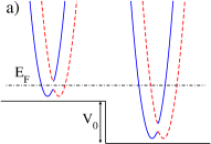
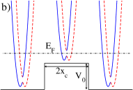
Figure 1: (Color online) a) A potential step of height $V_{0}$ and b) a potential barrier of height $V_{0}$ and width $2x_{c}$. The corresponding dispersions in the different regions are sketched (solid line: $s=+$, dashed line: $s=-$).

As an additional effect of the magnetic field, the spin expectation value is rotated gradually from the $\pm y$-direction into the $\pm x$-direction when $|k|\to 0$, while $\left<\sigma_{z}\right>_{k,s}$ remains zero. Depending on the chosen parameters, this leads to a small $x$-component of the ground state magnetization, whereas the $y$- and $z$-components are exactly zero as will be explained below.

We here generalize the situation studied in Ref. streda, in several ways. We first study how the above scenario is modified in the presence of an additional Rashba term

$$H_{R}^{\prime}=\frac{\hbar}{m}\alpha_{y}\sigma_{z}p_{x}$$ (4)

resulting from the confinement of the 2DEG to the wire geometry, a term which so far was mainly ignored. As we also focus on the lowest subband and do not study subband mixing, the exact shape of the potential confining the electrons to the wire is not important. As its main effect, $H_{R}^{\prime}$ will lead to nonvanishing spin expectation values $\langle\sigma_{z}\rangle_{k,s}$ and thus a spin polarization component perpendicular to the plain of the underlying 2DEG. We also study the transmission current and the spin polarization at a potential barrier and discuss the interplay of $\alpha_{y}$ and $\alpha_{z}$. In addition, we present a lattice model which in an appropriate parameter regime shows the same physics as the continuum model. This model will allow us to study the effect of the electron-electron interaction on the spin polarization in a forthcoming publicationinteractionpaper using the functional renormalization group method.funRG

II Continuum model

The model we consider is given by the Hamiltonian

$$H=\frac{p_{x}^{2}}{2m}-\frac{\hbar\alpha_{z}}{m}\sigma_{y}p_{x}+\frac{\hbar\alpha_{y}}{m}\sigma_{z}p_{x}-\frac{e\hbar}{2mc}\mbox{\boldmath{$\sigma$}}\cdot\mathbf{B}\;.$$ (5)

We slightly generalized the situation discussed above and allow for a Zeeman term with a magnetic field $\mathbf{B}=B(\sin{\theta}\cos{\varphi},\sin{\theta}\sin{\varphi},\cos{\theta})$ pointing in arbitrary direction. The normalized eigenstates with quantum numbers $k$ and $s=\pm$ are given by the product of a plane wave (in $x$-direction) and a two-component spinor

$$\phi_{k}^{(s)}(x)=\frac{\displaystyle{1}}{\displaystyle\sqrt{2\pi}}e^{ikx}\left(\begin{array}[]{c}A_{k}^{(s)}\\ B_{k}^{(s)}\end{array}\right)\,.$$ (6)

Applying the Hamiltonian Eq. (5) to this ansatz we obtain

$$\left(\begin{array}[]{c c}k^{2}+2\alpha_{y}k+2k_{Z}^{2}\cos\theta-\epsilon,&2ik\alpha_{z}+2k_{Z}^{2}e^{-i\varphi}\sin\theta\\ 2ik\alpha_{z}+2k_{Z}^{2}e^{i\varphi}\sin\theta,&k^{2}-2\alpha_{y}k-2k_{Z}^{2}\cos\theta-\epsilon\end{array}\right)\left(\begin{array}[]{c}A_{k}^{(s)}\\ B_{k}^{(s)}\end{array}\right)=0\,,$$ (7)

with $\epsilon=2mE/\hbar^{2}$, $\alpha_{y}=eE_{y}/(4mc^{2})$, $\alpha_{z}=eE_{z}/(4mc^{2})$, and $k_{Z}^{2}=-eB/(2\hbar c)$. Note that $\alpha_{y},\alpha_{z}<0$ in our notation due to the negative electron charge. One obtains the eigenenergy (divided by $\hbar^{2}/2m$)

$$\epsilon^{(s)}(k)=k^{2}+2s\operatorname{sgn}(k-k_{0})\sqrt{C(k)}\,,$$ (8)

with $C(k)=(\alpha_{y}^{2}+\alpha_{z}^{2})k^{2}+2k_{Z}^{2}k(\alpha_{y}\cos\theta-\alpha_{z}\sin\theta\sin\varphi)+k_{Z}^{4}$ and $k_{0}=-k_{Z}^{2}\left(\alpha_{y}\cos\theta-\alpha_{z}\sin\theta\sin\varphi\right)/(\alpha_{y}^{2}+\alpha_{z}^{2})$ being the wave number at which the “energy gap” becomes smallest [see Fig. 2]. The corresponding eigenfunctions are

$$\phi_{k}^{(s)}(x)=\frac{1}{\sqrt{2\pi}\sqrt{1+\left|a_{k}^{(s)}\right|^{2}}}e^{ikx}\left(\begin{array}[]{c}a_{k}^{(s)}\\ 1\end{array}\right)\,,$$ (9)

$$\mbox{with}\quad a_{k}^{(s)}=\frac{-i\alpha_{z}k-k_{Z}^{2}e^{-i\varphi}\sin\theta}{\alpha_{y}k+k_{Z}^{2}\cos\theta-s\operatorname{sgn}(k-k_{0})\sqrt{(\alpha_{y}^{2}+\alpha_{z}^{2})k^{2}+2k_{Z}^{2}k(\alpha_{y}\cos\theta-\alpha_{z}\sin\theta\sin\varphi)+k_{Z}^{4}}}$$ (10)

and the spin expectation values are given by

$$\langle\sigma_{x}+i\sigma_{y}\rangle_{k,s}=2\frac{\left(a_{k}^{(s)}\right)^{*}}{1+\left|a_{k}^{(s)}\right|^{2}}\,,\quad\langle\sigma_{z}\rangle_{k,s}=\frac{-1+\left|a_{k}^{(s)}\right|^{2}}{1+\left|a_{k}^{(s)}\right|^{2}}\,.$$ (11)

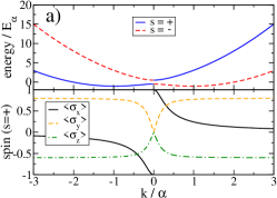
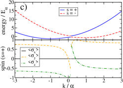
Figure 2: (Color online) Dispersion and spin expectation values on the ($s=+$)-branch for a magnetic field in a) $x$- , b) $y$- and c) $z$-direction, $\alpha_{y}/\alpha=-0.6$, $\alpha_{z}/\alpha=-0.8$, $k_{Z}/\alpha=0.5$. The spin on the ($s=-$)-branch points in the opposite direction, i.e. $\langle\sigma_{i}\rangle_{k,s}=-\langle\sigma_{i}\rangle_{k,-s}$. The shape of the dispersion and the $k$-value at which the “energy gap” becomes smallest clearly depends on the direction of the magnetic field.

As can be seen from Eq. (11), the necessary condition $\langle\sigma_{x}\rangle^{2}_{k,s}+\langle\sigma_{y}\rangle^{2}_{k,s}+\langle\sigma_{z}\rangle^{2}_{k,s}=1$ holds for all values of $s$ and $k$. The existence of the confinement in $y$-direction (represented by $\alpha_{y}$) leads to a rotation of the spin out of the $x$-$y$-plain into the $z$-direction. This indicates that the ratio of $\alpha_{y}$ and $\alpha_{z}$ is crucial for the spin direction.

The energy dispersion Eq. (8) and the spin expectation values on the ($s=+$)-branch are shown in Fig. 2 as a function of $k$, with $k$ given in units of $\alpha=\sqrt{\alpha_{y}^{2}+\alpha_{z}^{2}}$ and the energy in units of $E_{\alpha}=\hbar^{2}\alpha^{2}/2m$. For $|k|\gtrsim\alpha$ the spin expectation values reach their asymptotic, $k$-independent values. The spin on the ($s=-$)-branch points in the opposite direction, i.e. $\langle\sigma_{i}\rangle_{k,s}=-\langle\sigma_{i}\rangle_{k,-s}$, and is not shown explicitly here. In combination with the fact that for $\mathbf{B}=(B,0,0)$, $\langle\sigma_{y}\rangle_{k,s}$ and $\langle\sigma_{z}\rangle_{k,s}$ are symmetric with respect to $k=0$ on both branches, this explains why there is no ground state magnetization in the $y$- and $z$-direction for $\mathbf{B}$ being parallel to the wire. However, there is a nonvanishing ground state magnetization in the $x$-direction. The “energy gap” is given by $4\sqrt{C(k_{0})}$ [see Eq.(8)] and does not necessarily decrease from its maximum value $4k_{Z}^{2}$, if $\mathbf{B}$ is tilted against $\mathbf{e}_{x}$ as stated in Ref. streda, . In units of the Zeeman energy $E_{Z}=2\hbar^{2}k_{Z}^{2}/2m$, the size of the “gap” $E_{G}$ for arbitrary magnetic field $\mathbf{B}=B(\sin\theta\cos\phi,\sin\theta\sin\phi,\cos\theta)$ is given by

$$\frac{E_{G}}{E_{Z}}=1-\frac{\left(\alpha_{y}\cos\theta-\alpha_{z}\sin\theta\sin\phi\right)^{2}}{\alpha^{2}}.$$ (12)

Therefore, a finite $\alpha_{y}$ term is necessary for opening the “gap” for $\mathbf{B}||\mathbf{e}_{y}$. To emphasize this effect, we choose the parameter set $(\alpha_{y},\alpha_{z},k_{Z})/\alpha=(-0.6,-0.8,0.5)$ in Fig. 2. In many experimental systems the confining potential in the $y$-direction might be much weaker than in the $z$-direction. In this case $|\alpha_{y}|\ll|\alpha_{z}|$ but subband mixing becomes relevant. The latter strongly affects the spin-dependent transport properties as e.g. investigated in Ref. uli, , and the polarization effects discussed here can be expected to disappear. To achieve spin polarization in the present setup a strong confinement in the $y$-direction leading to a sizable $\alpha_{y}$ is thus essential. The lower dispersion branch in Fig. 2 has a “W”-like shape. For $\mathbf{B}=(B,0,0)$, the condition for this behavior is $\alpha_{y}^{2}+\alpha_{z}^{2}>2k_{Z}^{2}$ and becomes much more complex for arbitrary magnetic field. We will focus on the situation where $\mathbf{B}=(B,0,0)$.

The transmissions $t_{ss^{\prime}}$ (conductance divided by $e^{2}/\hbar$) of an electron current at fixed Fermi energy $E_{F}$ passing a potential step in the wire direction [see Fig. 1 a)] are obtained by assuming continuity of the wave functions and their derivatives at the interface. Here the first index labels the branch to the left and the second index labels the branch to the right of the potential step. It was argued in Ref. molenkamp, that one has to consider the continuity of the wave function’s flux and not simply its derivative, but in our setup both conditions lead to the same equations as we consider a homogeneous SOI. The total transmission $T$ is the sum of the four components $t_{++}$, $t_{+-}$, $t_{-+}$, and $t_{--}$. To the right of the potential and for momenta $|k|\gtrsim\alpha$, one can assign spins with quantum numbers $\uparrow,\downarrow$ and a properly chosen quantization axis to the branches $s=+,-$ because of the independence of $\langle\mbox{\boldmath{$\sigma$}}\rangle_{k,s}$ on $k$. However, the polarization vector is given by

$$\mathbf{P}=\frac{t_{++}+t_{-+}}{T}\langle\mbox{\boldmath{$\sigma$}}\rangle_{k,+}+\frac{t_{+-}+t_{--}}{T}\langle\mbox{\boldmath{$\sigma$}}\rangle_{k,-}\,.$$ (13)

Since the potential step geometry was already discussed,streda we will only shortly mention the influence of the additional term $H_{R}^{\prime}$, defined in Eq. (4), and discuss the interesting case of a potential barrier [see Fig. 1 b)] in more detail. The latter can experimentally be achieved by adding gates to the 1D quantum wire.

As shown in Fig. 3, the total polarization $P=|\mathbf{P}|$ of the current passing the potential step is large for energies in the “gap” and increases with $\alpha$. Similar to the transmissions $t_{ss^{\prime}}$, $P$ as well as the parallel polarization $P_{x}$ depend only on $V_{0}$, $k_{Z}$, and $\alpha$ for $\mathbf{B}||\mathbf{e}_{x}$ and not on $\alpha_{y}$ and $\alpha_{z}$ independently. The relevant energy scale of the polarization shown in Fig. 3 is given by $E_{Z}$, which defines the size of the “gap” [see Eq. (12)]. Therefore, energies are given in units of $E_{Z}$ and wave vectors in units of $k_{Z}$. The same holds for the transmissions and polarizations shown further down (see Figs. 4 and 5). The parameters in Fig. 3 are $V_{0}/E_{Z}=15$, and $\alpha/k_{Z}=2$, $2.5$, $3$, $5$. The energy offset is chosen such that $E_{F}/E_{Z}=0$ corresponds to the middle of the “gap”. The parallel polarization $P_{x}$ gives the main contribution to the total polarization as the energy departs from the “gap”, $P_{x}/P\rightarrow 1$. However, in this region the total polarization is negligible and within the “gap”, the parallel component plays an inferior role. The ratio of the two perpendicular polarizations is given by $\left|P_{z}/P_{y}\right|=\alpha_{y}/\alpha_{z}$. Therefore, the orthogonal polarization $\mathbf{P}_{\perp}=(0,P_{y},P_{z})$ can be rotated within the $y$-$z$-plane by adjusting $\alpha_{y}$ and $\alpha_{z}$.

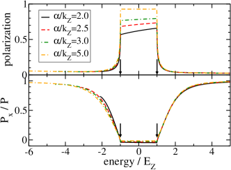
Figure 3: (Color online) Polarization of the transmission current at a potential step as a function of the Fermi energy for $V_{0}/E_{Z}=15$ and $\alpha/k_{Z}=2$, $2.5$, $3$, $5$. The total polarization $P$ is sizable for energies in the “gap” (indicated by the arrows). In this regime it is mostly carried by $P_{y}$ and $P_{z}$. The polarization becomes negligible for energies outside the “gap” where $P_{x}$ dominates.

We next study the transmission current at a potential barrier of height $V_{0}$ and width $2x_{c}$ [see Fig. 1 b)]. This situation might be more realistic than a simple potential step if one thinks of further structuring by applying gates to the quantum wire. Fig. 4 shows the four components of the transmission as a function of $E_{F}/E_{Z}$ for $\alpha/k_{Z}=2$, $2.5$, $3$, $V_{0}/E_{Z}=15$, and $k_{Z}x_{c}=1$. Again, the SOI affects the transmissions $t_{ss^{\prime}}$ only via $\alpha$. Interestingly and in contrast to the potential step, the $s$-flipping transmissions are degenerate, $t_{+-}=t_{-+}$. This can be understood, if one considers the possible $s$-flips at the two interfaces leading to an overall $s$-flip.

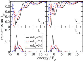
Figure 4: (Color online) Partial transmissions at a potential barrier as a function of the energy for $V_{0}/E_{Z}=15$ and $\alpha/k_{Z}=2$, $2.5$, $3$.

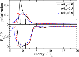
Figure 5: (Color online) Polarization of the transmission current at a potential barrier as a function of the energy for the same parameters as in Fig. 4. The polarization is sizable for energies well beyond the “gap” (indicated by the arrows) and shows oscillatory behavior. The $x$-component $P_{x}$ is only relevant in regimes where the total polarization is small.

Labeling the left interface (1) and the right (2), one simply has to take the sum of the products of transmissions at each interface and obtains

$$t_{+-} = t_{++}(1)t_{+-}(2)+t_{+-}(1)t_{--}(2)\,,$$

$$t_{-+} = t_{--}(1)t_{-+}(2)+t_{-+}(1)t_{++}(2)\,.$$ (14)

An analysis of the potential step problem shows that the $s$-conserving transmissions $t_{++}$ and $t_{--}$ are independent of the sign of $V_{0}$ and the $s$-flipping transmissions just swap, i.e. $t_{+-}(1)=t_{-+}(2)$ and $t_{-+}(1)=t_{+-}(2)$. This leads to exactly the same values of $t_{+-}$ and $t_{-+}$ in Eq. (14). The exponential suppression of $t_{++}(1)$ and $t_{-+}(1)$ for energies within the “gap” does not affect this behavior. The $s$-conserving transmissions $t_{++}$ and $t_{--}$ show an oscillatory behavior, which is well known from scattering off a potential step at vanishing SOI. However, especially for low energies, the amplitude strongly depends on $\alpha$. The $s$-flipping transmissions $t_{+-}$ and $t_{-+}$ oscillate as well. The second peak of $t_{++}$, which lies in the “energy gap”, is suppressed compared to $t_{--}$, since right-moving ($s=+$)-waves are exponentially damped in the barrier region and therefore, as shown in Ref. streda, , $t_{--}$ is the dominant component at each interface in this energy range.

Fig. 5 shows $P$ and $P_{x}/P$ for the same parameters as in Fig. 4. and $\alpha/k_{Z}=2$, $2.5$, $3$. Similarly to the potential step case, $P=|\mathbf{P}|$ and $P_{x}$ only depend on $\alpha$ and not on $\alpha_{y}$ and $\alpha_{z}$ independently. Surprisingly, the polarization now has a sizable value in an energy interval much bigger than the “gap”, which just goes from $-E_{Z}$ to $E_{Z}$ (see the arrows in Fig. 5). This behavior must be contrasted to the polarization in the case of a potential step as shown in Fig. 3 and first introduced in Ref. streda, . It can be traced back to the energy dependence of $t_{+-}$ and $t_{-+}$ shown in Fig. 4. Both have finite weight well beyond the “energy gap”. This might be due to interference effects of transmitted and reflected waves in the barrier region.

III Lattice model

In a next step, we are aiming at constructing a tight-binding lattice model which in appropriate parameter regimes shows similar physics as our continuum model. This will put us in a position to study the effect of electron-electron interaction neglected so far using the functional renormalization group method.funRG In 1D wires the two-particle interaction is known to strongly alter the low-energy physics of many-body systems leading to so called Luttinger liquid behavior.KS It can be expected that the interplay of the SOI effects discussed above and correlation effects leads to interesting physics.

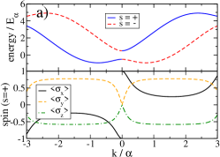
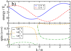
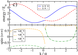
Figure 6: (Color online) Lattice dispersion and spin expectation values on the ($s=+$)-branch for a magnetic field in a) $x$- , b) $y$- and c) $z$-direction for $t/\alpha=1$, $\alpha_{y}/\alpha=-0.6$, $\alpha_{z}/\alpha=-0.8$, $k_{Z}/\alpha=0.5$. The spin on the ($s=-$)-branch points in the opposite direction, i.e. $\langle\sigma_{i}\rangle_{k,s}=-\langle\sigma_{i}\rangle_{k,-s}$. For $\left|k-k_{0}\right|<\pi/2$ one obtains exactly the same behavior as in the continuum case.

The SOI can be modeled by spin-flip hopping terms with amplitude $\alpha_{y}$ and $\alpha_{z}$ in a usual tight-binding model.mireles

We start with a representation of the Hamiltonian in terms of Wannier states $|j,\sigma\rangle$ with $j\in\mathbb{Z}$ labeling the lattice site and $\sigma=\uparrow,\downarrow$ labeling the spin. The spin quantization is chosen along the $z$-direction. With $c_{j,\sigma}^{\dagger}$ being the creation operator of an electron at site $j$ with spin $\sigma$, the lattice model Hamiltonian for an arbitrary magnetic field $\mathbf{B}=B\left(\sin\theta\cos\varphi,\sin\theta\sin\varphi,\cos\theta\right)$ can be written as

$$H=H_{0}+H_{\mathrm{pot}}+H_{R}+H_{Z}\,,$$ (15)

with the free part

$$H_{0}=\epsilon\sum_{j,\sigma}c_{j,\sigma}^{\dagger}c_{j,\sigma}-t\sum_{j,\sigma}\left(c_{j+1,\sigma}^{\dagger}c_{j,\sigma}+c_{j,\sigma}^{\dagger}c_{j+1,\sigma}\right)\,,$$ (16)

containing the on-site energy and the conventional (spin-conserving) hopping, external potential (due to e.g. nano-device structuring)

$$H_{\mathrm{pot}}=\sum_{j,\sigma}V_{j,\sigma}c_{j,\sigma}^{\dagger}c_{j,\sigma}\,,$$ (17)

the spin-flip (Rashba) hopping terms

$$H_{R} = -\alpha_{z}\sum_{j,\sigma,\sigma^{\prime}}\left(c_{j+1,\sigma}^{\dagger}\left(i\sigma_{y}\right)_{\sigma,\sigma^{\prime}}c_{j,\sigma^{\prime}}+\mbox{H.c.}\right)$$

$$+\alpha_{y}\sum_{j,\sigma,\sigma^{\prime}}\left(c_{j+1,\sigma}^{\dagger}\left(i\sigma_{z}\right)_{\sigma,\sigma^{\prime}}c_{j,\sigma^{\prime}}+\mbox{H.c.}\right)\,,$$

and the Zeeman term

$$H_{Z} = 2k_{Z}^{2}\sum_{j,\sigma,\sigma^{\prime}}c_{j,\sigma}^{\dagger}\left[\left(\sigma_{x}\right)_{\sigma,\sigma^{\prime}}\sin\theta\cos\varphi\right.$$

$$+\left.\left(\sigma_{y}\right)_{\sigma,\sigma^{\prime}}\sin\theta\sin\varphi+\left(\sigma_{z}\right)_{\sigma,\sigma^{\prime}}\cos\theta\right]c_{j,\sigma^{\prime}}\,.$$

We show the analogy to the continuum case suppressing $H_{\mathrm{pot}}$ and take as an ansatz for the corresponding eigenstates

$$|k,s\rangle=\sum\limits_{j,\sigma}a_{\sigma}^{s}(k)e^{ikj}|j,\sigma\rangle\,.$$ (20)

This leads to the eigenenergies

$$E^{(s)}(k)=\epsilon-2t\cos k+2s\operatorname{sgn}(k-k_{0})\sqrt{D(k)}\,,$$ (21)

with

$$k_{0}=\arcsin\left[-k_{Z}^{2}(\alpha_{y}\cos\theta-\alpha_{z}\sin\theta\sin\varphi)/(\alpha_{y}^{2}+\alpha_{z}^{2})\right]$$ (22)

and

$$D(k) = (\alpha_{y}^{2}+\alpha_{z}^{2})\sin^{2}k+k_{Z}^{4}$$

$$+2k_{Z}^{2}\sin k\left(\alpha_{y}\cos\theta-\alpha_{z}\sin\theta\sin\varphi\right)\,.$$

Eq. (21) has almost the same form as the continuum version Eq. (8). In fact, choosing the on-site energy $\epsilon=2t$, which corresponds just to an overall energy shift, and substituting $\cos k$ by $1-k^{2}/2$ and $\sin k$ by $k$, which is valid for sufficiently small $|k|$, we get exactly the same form. Note however that, in contrast to the continuum case, $\alpha_{y},\alpha_{z}$ and $k_{Z}^{2}$ now have the unit of energy, but since $c_{k}^{(s)}$, defined in Eq. (24) is dimensionless, all formulas remain valid. We choose for the eigenstates Eq. (20) $a_{\downarrow}^{s}(k)=1$ and obtain $a_{\uparrow}^{s}(k)=c_{k}^{(s)}$

$$\mbox{with}\quad c_{k}^{(s)}=\frac{-i\alpha_{z}\sin k-k_{Z}^{2}e^{-i\varphi}\sin\theta}{\alpha_{y}\sin k+k_{Z}^{2}\cos\theta-s\operatorname{sgn}(k-k_{0})\sqrt{(\alpha_{y}^{2}+\alpha_{z}^{2})\sin^{2}k+2k_{Z}^{2}\sin k(\alpha_{y}\cos\theta-\alpha_{z}\sin\theta\sin\varphi)+k_{Z}^{4}}},$$ (24)

and the spin expectation values have exactly the continuum form

$$\langle\sigma_{x}+i\sigma_{y}\rangle_{k,s}=2\frac{\left(c_{k}^{(s)}\right)^{*}}{1+\left|c_{k}^{(s)}\right|^{2}},\quad\langle\sigma_{z}\rangle_{k,s}=\frac{-1+\left|c_{k}^{(s)}\right|^{2}}{1+\left|c_{k}^{(s)}\right|^{2}}\,.$$ (25)

The energy dispersions and the spin expectation values for magnetic fields in $x$-, $y$-, and $z$-direction are shown in Fig. 6. Besides the cosine-like structure, which becomes especially relevant near the band edges, the dispersion and spin expectation values have the same shape as in the continuum model. A direct comparison of Fig. 6 and Fig. 2 shows that our lattice model reproduces the low energy physics, i.e. for $\left|k-k_{0}\right|<\pi/2$, observed in the continuum. As above we only show the spin expectation values on the ($s=+$)-branch. The spin on the ($s=-$)-branch points in the opposite direction, i.e. $\langle\sigma_{i}\rangle_{k,s}=-\langle\sigma_{i}\rangle_{k,-s}$. The direct relation between the dispersion and the spin expectation values for energies of the order of the “gap” is the essential feature leading to the remarkable scattering properties of the continuum model (and eventually a spin polarized conductance) at steps and barriers. One can thus expect similar transport characteristics to be realized in the lattice model. A detailed discussion of this and in particular the effect of the electron-electron interaction on transport will be the topic of an upcoming publication.interactionpaper

IV Conclusions

We have investigated the dispersion and spin expectation values of a 1D electron system with SOI as well as arbitrary magnetic field, and have shown that an additional SOI term resulting from the lateral confinement of a 2DEG to a 1D wire geometry leads to a rotation of the spin out of the 2D plane. For the case of a magnetic field parallel to the quantum wire, the transmission and polarization of a linear response current at a potential step as well as at a potential barrier were studied. For the latter, we observed an extended energy range, where significant spin polarization can be achieved. We showed that this spin polarization can be rotated out of the plane of the 2DEG arbitrarily by adjusting the SOI constants $\alpha_{y}$ and $\alpha_{z}$. The potential barrier describes a setup which can experimentally be achieved by adding further gates to the wire geometry. We then constructed a lattice model which shows the same low energy physics as the continuum model. This lattice model now enables us to investigate the interplay of SOI and Coulomb interaction in quantum wires with potential steps and barriers using the functional renormalization group method.interactionpaper ; funRG

References

- (1) I. Žutić, J. Fabian, and S. Das Sarma, Rev. Mod. Phys. 76, 323 (2004).
- (2) R. Winkler, Spin-Orbit Coupling Effects in Two-Dimensional Electron and Hole Systems, Springer-Verlag, Berlin (2003).
- (3) E.I. Rashba, Physica E 34, 31 (2006).
- (4) The SOI coupling coefficients are assumed to be independent from the coordinates , i.e. , with and .
- (5) S. Datta and B. Das, Appl. Phys. Lett. 56, 7 (1990).
- (6) A.V. Moroz and C.H.W. Barnes, Phys. Rev. B 60, 14272 (1999).
- (7) F. Mireles and G. Kirczenow, Phys. Rev. B 64, 24426 (2001).
- (8) M. Governale and U. Zülicke, Phys. Rev. B 66, 07331 (2002); Solid State Com. 131, 581 (2004).
- (9) P. Strěda and P. Sěba, Phys. Rev. Lett. 90, 256601 (2003).
- (10) R.G. Pereira and E. Miranda, Phys. Rev. B 71, 085318 (2005).
- (11) L. Serra, D. Sánchez, and R. López, Phys. Rev. B 72, 235309 (2005).
- (12) S. Zhang, R. Liang, E. Zhang, L. Zhang, and Y. Liu, Phys. Rev. B 73, 155316 (2006).
- (13) J.E. Birkholz and V. Meden, in preparation.
- (14) S. Andergassen, T. Enss, V. Meden, W. Metzner, U. Schollwöck, and K. Schönhammer, Phys. Rev. B 73, 045125 (2006).
- (15) L.W. Molenkamp, G. Schmidt, and G.E.W. Bauer, Phys. Rev. B 64, 121202 (2001).
- (16) For a recent review see K. Schönhammer in Interacting Electrons in Low Dimensions, Ed.: D. Baeriswyl, Kluwer Academic Publishers (2005).