Exact Solutions of the Equations of Relativistic Hydrodynamics

Exact Solutions of the Equations of Relativistic
Hydrodynamics Representing Potential Flows

Maxim S. BORSHCH and Valery I. ZHDANOV

M.S. Borshch and V.I. Zhdanov

National Taras Shevchenko University of Kyiv, Ukraine unacabeza@ukr.net, zhdanov@observ.univ.kiev.ua http://www.observ.univ.kiev.ua/astrophysics/zhdanov/

Received September 10, 2007, in final form November 28, 2007; Published online December 07, 2007

We use a connection between relativistic hydrodynamics and scalar field theory to generate exact analytic solutions describing non-stationary inhomogeneous flows of the perfect fluid with one-parametric equation of state (EOS) $p=p(\varepsilon)$. For linear EOS $p=\kappa\varepsilon$ we obtain self-similar solutions in the case of plane, cylindrical and spherical symmetries. In the case of extremely stiff EOS ($\kappa=1$) we obtain “monopole $+$ dipole” and “monopole $+$ quadrupole” axially symmetric solutions. We also found some nonlinear EOSs that admit analytic solutions.

relativistic hydrodynamics; exact solutions

76Y05; 83C15; 83A05

1 Introduction

Relativistic hydrodynamics (RHD) is extensively used to describe various processes from microscopic to cosmological scales. Astrophysical applications of RHD deal with powerful non-stationary phenomena such as the gamma-ray bursts and hypernovae explosions. On the other hand, RHD solutions are sources of hydrodynamical models of elementary particle multiple production. Though at present there are powerful methods to find numerical solutions of hydrodynamical problems, the price for exact analytic representations of RHD flows is still high. However, the nonlinear structure of the RHD equations hampers the quest of analytic solutions and this is the reason why RHD problems having exact solutions typically deal with simple equation of state (EOS) such as $p=\kappa\varepsilon$ ($p$ is the pressure, $\varepsilon$ is the proper frame energy density, $\kappa={\rm const}$). This linear equation of state is often used in multiple pion production theory since works of Landau [2] and Khalatnikov [3].

The most part of known exact RHD solutions concerns plane ($1+1$ dimensional) barotropic relativistic flows. The Riemann simple waves are the example (see, e.g., [4]). In the case of the linear EOS the method of Khalatnikov [3] allows to obtain a general solution in an implicit form. However, the solutions obtained by means of this method have rather complicated representation. This motivated different authors to look for more simple solutions to be used in models of multiple pion production [6, 7, 8, 9]; these solutions have extensions to the case of spherical and cylindric symmetry. Recent interest to such solutions is due to high energy heavy ion collisions (see, e.g., [10, 11, 12]).

The three-dimensional case of RHD is less developed. No general analytic solution is known in the case of relativistic spherically symmetric flows as well as in the case of cylindric symmetry. The best known in theory of astrophysical relativistic outbursts is the Blandford & McKee approximate self-similar solution [13] that describes ultra-relativistic blast waves of the fluid with the linear EOS; for modifications and generalizations (also in the ultra-relativistic approximation) see [14, 15].

Various techniques were invented in classical hydrodynamics in order to find analytic solutions. In particular, one may consider potential flows of ideal fluid to reduce the number of unknown functions. In this paper we study RHD flows that may be considered as a relativistic analog of the classical potential flow: in these flows the four-velocity is proportional to a gradient of a scalar function. The relation between RHD flows and the scalar fields is well known (see, e.g., [5, 7, 16]) and at present it may be considered as a part of physical folklore. This relation is extensively used in cosmology in connection with the dark energy problem [17, 18, 19, 20]. Here a number of unusual equations of state has appeared; they have been considered in the context of spatially homogeneous cosmological systems (see, e.g., [20] for the review).

In this paper we use the connection between RHD and the scalar field theory that allows us to reduce the problem to an equation for a single scalar function (instead of four-velocity and energy density). The aim of this paper is to study the ability of this trick to generate analytic RHD solutions that represent non-stationary and non-homogeneous flows of relativistic perfect fluid. The paper is organized as follows. In Section 2 we present basic equations and relations between the scalar field and hydrodynamical variables. In Section 3 we present solutions for an extremely stiff EOS: there are plane solutions, spherical solutions including different combination of outgoing and ingoing spherical waves; at last we present examples of three-dimensional solutions that are obtained from spherical harmonics of the scalar field. In Section 4 we present some nonlinear equations of state that allow us to find exact RHD solutions. In Section 5 we present two families of self-similar solutions in the case of the linear EOS. In summary we briefly discuss the results obtained, their relation to the other known solutions and possible generalizations.

2 Notations and basic equations

The relativistic equations of the perfect fluid dynamics may be written as conservation laws (e.g., [21]):

$$\partial_{\nu}T^{\mu\nu}=0,$$ (1)

where

$$T^{\mu\nu}=\left({p+\varepsilon}\right)\,u^{\mu}u^{\nu}-pg^{\mu\nu},\qquad u^{\mu}u_{\mu}=1,\qquad g_{\mu\nu}={\rm diag}\,\left({1,-1,-1,-1}\right);$$ (2)

$u^{\mu}$ is the four-velocity, $p$ is the pressure and $\varepsilon$ is the proper frame energy density, the Greek indices run from 0 to 3, the speed of light $c=1$. In the general case equation (1) must be supplemented with the baryon number conservation equations. However, it is not necessary in this paper because we deal only with the one-parametric EOS $p=p(\varepsilon)$; provided EOS be known, the system (1) is complete. Further we concretize different equations of state in every section.

If we have a conserved energy-momentum tensor of any field with known solutions, we can use it to find a hydrodynamic solutions for $\varepsilon$, $u^{\mu}$. However, to do this one needs to represent this energy-momentum tensor in the form (2); moreover, in order that these solutions represent physically admissible motion of the relativistic fluid one must provide the time-like behavior of the four-velocity. This is not always possible. However, solutions with a spacelike $u^{\mu}$ are also of some interest: they demonstrate that formal solutions of completely relativistic dynamical equations may admit tachyonic motions.

Transition to the proper frame of a local fluid element shows that arbitrary tensor can be represented in the form (2), if the matrix $T^{\mu}_{\nu}$ has only one eigenvalue $\varepsilon>0$ corresponding to a timelike eigenvector and triple-degenerate eigenvalue $p$ with space-like eigenvectors. It is not always possible to fulfill these requirements for an arbitrary $T^{\mu}_{\nu}$. However in the case of a scalar field with the Lagrangian

$$L=F(S),\qquad S=\frac{1}{2}\varphi_{,\alpha}\varphi_{,}^{\;\alpha}$$ (3)

the corresponding energy-momentum tensor

$$T_{\alpha\beta}=\varphi_{,\alpha}\varphi_{,\beta}F^{\prime}(S)-g_{\alpha\beta}F(S)$$

takes on the form (2), if we put [5]:

$$p=F(S),\qquad\varepsilon=2SF^{\prime}(S)-F(S),$$ (4)

$$u_{\alpha}=\pm\varphi_{,\alpha}(2S)^{-1/2}.$$ (5)

The equations (4) provide an effective EOS that is represented parametrically.

The equation of the scalar field following from (3) is

$$\partial_{\alpha}[F^{\prime}(S)\partial^{\alpha}\varphi]=0.$$ (6)

Formulae (4), (5) represent an admissible hydrodynamic flow provided that

$$\varepsilon>0,\qquad S>0.$$ (7)

This is the only condition to check, if we have a solution of equation (6).

3 Extremely stiff EOS: plane and spherical solutions

3.1 Plane solutions

The most simple is the case of a massless scalar field corresponding to the extremely stiff EOS:

$$F(S)=S,\qquad p=\varepsilon=S.$$

This EOS is considered throughout the whole section. In this case we deal with a linear wave equation for the scalar field:

$$\partial_{\mu}\partial^{\mu}\varphi=0.$$ (8)

In the case of plane symmetry $(x^{0}=t,\,x^{1}=x)$ it is easy to see that the general solution $\varphi=\psi\left({t-x}\right)+\chi\left({t+x}\right)$ admits a hydrodynamics interpretation if only

$$\psi^{\prime}\left({t-x}\right)\chi^{\prime}\left({t+x}\right)>0;$$ (9)

this makes it evident that the solutions corresponding to the only simple wave moving in one direction have no hydrodynamical counterpart. For hydrodynamical variables we have

$$v=\frac{u^{1}}{u^{0}}=-\frac{\partial\varphi/\partial x}{\partial\varphi/\partial t}=\frac{\psi\,^{\prime}\left({t-x}\right)-\chi^{\prime}\left({t+x}\right)}{\psi\,^{\prime}\left({t-x}\right)+\chi^{\prime}\left({t+x}\right)},\qquad\varepsilon=2\psi\,^{\prime}\left({t-x}\right)\chi^{\prime}\left({t+x}\right).$$ (10)

For $\psi^{\prime}\left(x\right)=\chi^{\prime}\left(x\right)=Ax^{-1}$ (throughout the paper $A={\rm const}\in{\mathbb{R}}$, $A\neq 0$) we obtain the scaling solutions [6, 7, 8, 9]: $v=x/t$, $\varepsilon=2A^{2}(t^{2}-x^{2})^{-1}$ that are well defined inside the light cone: $|x|<t$. For $x>t>0$ the hydrodynamical interpretation fails. If the solution for $t=t_{1}$, $|x|<x_{1}<t_{1}$ is considered as initial data for further hydrodynamic evolution, either the solution must be complemented by correct hydrodynamic data for $|x|>x_{1}$, or the equations must be modified (cf., e.g., [22, 23]) to extend the solution for all $x$. Note also that after rescaling $A\to iA$ we obtain a formal “tachyonic” solution outside the light cone with $\varepsilon>0$, but with $v>1$.

Choice $\psi^{\prime}\left(x\right)=\chi^{\prime}\left(x\right)=Ax^{\lambda}$, $|x|<t$ (here and below $\lambda\in{\mathbb{R}}$, $\lambda\neq 0$), generates similar solutions with the energy density $\varepsilon=2A^{2}(t^{2}-x^{2})^{\lambda}$ and $|v|<1$. For $\lambda<0$ we have an outflow ($v>0$); this solution is singular at the light cone. For positive $\lambda$ we have an inflow ($v<0)$; in particular, for positive even $\lambda$ the energy density has no light cone singularity. Simple rescaling of factors in the functions $\psi$, $\chi$ generates physical or tachyonic flows correspondingly inside or outside the light cone.

In order to construct a physical flow outside the light cone one can choose $\chi^{\prime}\left(x\right)=\psi^{\prime}\left(-x\right)=Ax^{\lambda}$, $x>t>0$. We have an outflow for $\lambda<0$, inflow for $\lambda>0$. This case can be easily extended to negative $x$ and/or to negative $t$. For $\lambda=1$ we obtain $\varepsilon=2A^{2}(x^{2}-t^{2}),\,v=-t/x$. This is a kind of external scaling solutions discussed in the papers [10, 11]. In order to obtain strict inequality (9) and regular solutions $\forall\,x,\,t$, the above power-law choice for $\psi$ and $\chi$ may be replaced, e.g., by $\chi^{\prime}\left(x\right)=\psi^{\prime}\left(-x\right)\sim\exp(\gamma x^{n})$, where $\gamma={\rm const}\in{\mathbb{R}}$, $n$ is a positive integer.

3.2 Spherical solutions

The general solution in the case of spherically symmetry ($x^{0}=t,\;x^{1}=r)$ is

$$\varphi=r^{-1}\left[{\psi\left({t-r}\right)+\chi\left({t+r}\right)}\right],$$

where $\psi$ and $\chi$ are arbitrary functions. Here, as distinct from the planar case, it is possible to use the outgoing wave solutions (with $\chi=0)$:

$$\varphi=\frac{\psi\left({t-r}\right)}{r},$$ (11)

whence

$$p=\varepsilon=-\frac{\psi^{2}}{2r^{4}}\left[{1+\frac{{2r\psi}^{\prime}}{\psi}}\right],\qquad v=1+\frac{\psi}{r{\psi}^{\prime}}.$$

In order to provide (7), it is necessary

$$2\frac{{\psi}^{\prime}\left(\alpha\right)}{\psi\left(\alpha\right)}r<-1,\qquad\alpha=t-r,$$ (12)

therefore the function $|\psi\left(\alpha\right)|$ is decreasing. Evidently it is impossible the condition (12) to hold for all $t$, $r$ (in particular, it is violated for $r\to 0$) and the hydrodynamical interpretation of $T_{\mu\nu}$ corresponding to the solution (11) is possible only in a bounded region. When the sign of $S$ changes and $\varepsilon=0$ this solution must be matched to vacuum in the way appropriate to hydrodynamic flow (see Appendix A).

Example. Consider a solution

$$\psi\left(\alpha\right)=C_{1}\alpha^{-n}-C_{2},$$

$C_{1}>0$ and $C_{2}>0$ being real constants, $n$ is positive integer. In this case (7) is fulfilled if

$$\psi+2r{\psi}^{\prime}=-\frac{\left[{\left({2n+1}\right)r-t}\right]C_{1}}{\alpha^{n+1}}-C_{2}<0.$$

This holds at least in the domain $\{(t,r):t>r>t/\left({2n+1}\right)\}$. As we see from Appendix A this solution is matched to vacuum for $t-r=t_{1}$, if $C_{1}t_{1}^{-n}=C_{2}$. For $r>t$ the hydrodynamical interpretation fails and it is either necessary to match the solution through a discontinuity, or the solution is destroyed by an external perturbation having trajectory $r=-t+{\rm const}$.

3.3 Combination of outgoing and ingoing spherical waves

In this case, in order to provide regularity of the solution for $r\to 0$, we put $\chi\left(t\right)=-\psi\left(t\right)$

$$\varphi\left({t,r}\right)=r^{-1}\left\{{\psi\left({t-r}\right)-\psi\left({t+r}\right)}\right\}.$$

Consider the power-law choice of $\psi\left(x\right)=-Ax^{-n}$, $A>0$, $n>0$. For every $n$ the inequalities (7) must be analyzed separately. Below we present the hydrodynamic solutions corresponding to four natural values of $n$; they have a hydrodynamic interpretation inside the light cone $t>r$.

For $n=1$, $t>r$:

$$\varphi=-\frac{2A}{t^{2}-r^{2}},\qquad\varepsilon=p=\frac{8A^{2}}{(t^{2}-r^{2})^{3}},\qquad v=\frac{r}{t}.$$ (13)

Appropriate rescaling of the constant $A$ yields a tachyonic solution outside the light cone.

For $n=2$, $t>r$:

$$\varphi=-\frac{4tA}{(t^{2}-r^{2})^{2}},\qquad\varepsilon=p=\frac{8A^{2}(9t^{2}-r^{2})}{(t^{2}-r^{2})^{5}},\qquad v=\frac{4tr}{3t^{2}+r^{2}}.$$ (14)

For $n=3$: $t>r$:

$$\varphi=-2A\frac{3t^{2}+r^{2}}{(t^{2}-r^{2})^{3}},\quad\varepsilon=p=\frac{32A^{2}(9t^{4}+2t^{2}r^{2}+r^{4})}{(t^{2}-r^{2})^{7}},\qquad v=\frac{r(5t^{2}+r^{2})}{3t(t^{2}+r^{2})}.$$ (15)

For $n=4$, $t>r$:

$$\varphi=-8A\frac{t(t^{2}+r^{2})}{(t^{2}-r^{2})^{4}},$$

$$\varepsilon=p=\frac{32A^{2}[10t^{4}(t^{2}+r^{2})+15t^{2}(t^{4}+t^{2}r^{2}+r^{4})-r^{6}]}{(t^{2}-r^{2})^{9}},\qquad v=\frac{2tr(3r^{2}+5t^{2})}{5t^{4}+10t^{2}r^{2}+r^{4}}.$$ (16)

In a more general case $(n\geq 1$, $A>0)$ one can show that hydrodynamic flow is correctly defined at least in the domain $\{(t,r):\kappa_{n}t<r<t\}$, where $\kappa_{n}=(a_{n}-1)/(a_{n}+1)$, $a_{n}=\left[2(n+1)\right]^{1/n}$, and in this region $u^{1}>0$.

4 Extremely stiff EOS: solutions based on spherical harmonics

In this section we proceed with the extremely stiff EOS; here generation of RHD solutions utilizes the well-known formula for the solution of the wave equation (8) using spherical functions $Y_{lm}\left({\theta,\varphi}\right)$ (in spherical coordinates)

$$\varphi\left({t,r,\theta,\varphi}\right)=\sum\limits_{l=0}^{\infty}{\;\sum\limits_{m=-l}^{l}{\;\tilde{f}_{lm}\left({t,r}\right)Y_{lm}\left({\theta,\varphi}\right)}},$$ (17)

$$\tilde{f}_{lm}=r^{l}\left({\frac{1}{r}\frac{\partial}{\partial r}}\right)^{l}\left\{{\frac{f_{lm}^{\left(1\right)}\left({t-r}\right)+f_{lm}^{\left(2\right)}\left({t+r}\right)}{r}}\right\},$$ (18)

where $f_{lm}^{\left(1\right)}\left({t-r}\right)$, $f_{lm}^{\left(2\right)}\left({t+r}\right)$ are arbitrary functions.

Investigation of inequality (7) for (17) is rather complicated in the general case. However, new special solutions obeying (7) may be easily obtained as follows. Take one of spherically symmetrical solutions (13)–(16) from the previous section and add some items from the sum in the r.h.s. of (17). These items must be sufficiently small in comparison with (13)–(16) to preserve inequality (7) at least within a compact domain inside the light cone. This is possible for a special choice of appropriate functions (18). Below we present two such special solutions that represent a hydrodynamical flow within the light cone $t>r$.

In the case of axial symmetry we obtain the three-dimensional velocity components from the relations

$$v^{r}\equiv\frac{u^{r}}{u^{0}}=-\frac{\varphi_{,r}}{\varphi_{,t}},\qquad v^{\theta}\equiv\frac{u^{\theta}}{u^{0}}=-\frac{1}{[r\sin(\theta)]^{2}}\frac{\varphi_{,\theta}}{\varphi_{,t}}.$$

The next case corresponds to the monopole + dipole contribution into $\varphi$:

$$\varphi=A\frac{t-br\cos\theta}{(t^{2}-r^{2})^{2}},$$

$b$ is a real constant. If $|b|<1$, then the condition (7) is satisfied for all $t>r$. Corresponding solution in terms of hydrodynamic variables is

$$\varepsilon=p=\frac{A^{2}}{2(t^{2}-r^{2})^{5}}\left[{(1-b^{2})(t^{2}-r^{2})+8\left({t-br\cos\theta}\right)^{2}}\right]>0,$$ (19)

$$v^{r}=\frac{4tr-(3r^{2}+t^{2})b\cos(\theta)}{3t^{2}+r^{2}-4trb\cos(\theta)},\qquad v^{\theta}=\frac{(t^{2}-r^{2})b\sin(\theta)}{r[3t^{2}+r^{2}-4trb\cos(\theta)]}.$$ (20)

The other solution is generated by a monopole $+$ quadrupole contribution

$$\varphi=A\frac{3t^{2}+r^{2}+br^{2}P_{2}}{(t^{2}-r^{2})^{3}},$$

where $P_{2}=[3\cos^{2}(\theta)-1]/2$, $b$ is a real constant. We checked that the condition (7) is also satisfied in this case for all $t>r$, at least if $|b|<1$. Corresponding hydrodynamical solution is

$$\varepsilon=p=\frac{A^{2}}{2(t^{2}-r^{2})^{7}}\big{[}{144t^{4}+16r^{2}(2t^{2}+r^{2})\left({1+2bP_{2}}\right)}$$

$$\phantom{\varepsilon=p=}{}-{2r^{2}b^{2}(P_{2}+1)(t^{2}-r^{2})+12b^{2}P_{2}^{2}r^{4}}\big{]}>0,$$ (21)

$$v^{r}=\frac{r}{3t}\frac{10t^{2}+2r^{2}+(t^{2}+2r^{2})bP_{2}}{2t^{2}+2r^{2}+br^{2}P_{2}},\qquad v^{\theta}=-\frac{b}{2t}\frac{(t^{2}-r^{2})\sin(\theta)\cos(\theta)}{2t^{2}+2r^{2}+br^{2}P_{2}}.$$ (22)

5 Nonlinear barotropic EOS

In this section we consider equation (6) in the case of plane ($n=0$), cylindrical ($n=1$) and spherical ($n=2$) symmetry. The dependence $p=p(\varepsilon)$ will be specified later. In this case equation (6) can be written as

$$\frac{\partial}{\partial t}\left({F^{\prime}(S)\frac{\partial\varphi}{\partial t}}\right)=\frac{1}{r^{n}}\frac{\partial}{\partial r}\left({r^{n}F^{\prime}(S)\frac{\partial\varphi}{\partial r}}\right).$$ (23)

We are looking for solutions of the equation (6) of the form

$$\varphi=\varphi(\sigma),\qquad\sigma=(t^{2}-r^{2})/2$$ (24)

In this case

$$S=\sigma\left(\frac{d\varphi}{d\sigma}\right)^{2}$$

and substitution into equation (23) yields

$$2\sigma\frac{d}{d\sigma}\left[F^{\prime}(S)\frac{d\varphi}{d\sigma}\right]+(2+n)F^{\prime}(S)\frac{d\varphi}{d\sigma}=0.$$ (25)

It is convenient to introduce a new variable $\tau$ by the relation $\sigma=\tau^{2}/2$; $S=(1/2)(d\varphi/d\tau)^{2}$. Then equation (25) yields

$${\tau^{1+n}F^{\prime}(S)}\frac{d\varphi}{d\tau}={\rm const}.$$ (26)

We investigate the most simple cases, when equation (26) can be easily solved with respect to $d\varphi/d\tau$ and the EOS is expressible in terms of elementary functions.

Consider first the EOS

$$p=\varepsilon\left[\ln\left(\frac{\varepsilon}{\varepsilon_{0}}\right)+B\right],\qquad F(x^{2}/2)=\varepsilon_{0}x[\ln(x)+B],$$ (27)

where $B$ is a dimensionless constant, $\varepsilon_{0}$ is a constant having the dimension of the energy density. Substitution into equation (26) gives us

$$\frac{d\varphi}{d\tau}=\exp\left(\frac{C}{\tau^{1+n}}-B-1\right),$$

$C$ being an arbitrary real constant. The solution of hydrodynamical equations with EOS (27) is

$$v=r/t,\qquad\varepsilon=\varepsilon_{0}\exp\left(\frac{C}{\tau^{1+n}}-B-1\right),\qquad\tau=\sqrt{t^{2}-r^{2}},\qquad t>r.$$ (28)

This solution is formally valid for interior of the future light cone. However, for usual hydrodynamical interpretation we need that

$$c_{s}^{2}=dp/d\varepsilon\in[0,1],$$ (29)

where $c_{s}$ is the speed of sound. This yields an additional restriction of the domain of RHD solution: $e^{-1}\leq\varepsilon e^{B}/\varepsilon_{0}\leq 1$ whence $t^{2}-r^{2}\geq C^{2/(1+n)}$, $C\geq 0$.

In a more complicated case we consider

$$F(S)=\varepsilon_{0}\sqrt{S}\sum\limits_{m=0}^{N}\frac{(-1)^{m}N!}{(N-m)!}\left(\ln\sqrt{S}\right)^{N-m}$$

with

$$\frac{dF}{dS}=\frac{\varepsilon_{0}}{2\sqrt{S}}\left(\ln\sqrt{S}\right)^{N}.$$

Corresponding EOS is represented parametrically ($R=\sqrt{S}$) as

$$\varepsilon=-\varepsilon_{0}R\sum\limits_{m=1}^{N}\frac{(-1)^{m}N!}{(N-m)!}\left(\ln R\right)^{N-m},\qquad p=\varepsilon_{0}R\sum\limits_{m=0}^{N}\frac{(-1)^{m}N!}{(N-m)!}\left(\ln R\right)^{N-m},$$ (30)

and both $\varepsilon$ and $p$ may be expressed as functions of enthalpy

$$\varepsilon+p=\varepsilon_{0}R\left(\ln R\right)^{N}.$$

In this case

$$c_{s}^{2}=\frac{dp}{d\varepsilon}=\frac{\ln R}{N}$$ (31)

On account of equation (26)

$$\tau^{1+n}\left(\ln R\right)^{N}={\rm const}.$$

This yields the hydrodynamical flow for the EOS (30) with

$$v=r/t,\qquad R=\exp\left[C(t^{2}-r^{2})^{-(1+n)/(2N)}\right],\qquad 0<r<t,$$ (32)

$C$ is a real constant. Taking into account of equations (31), (29) yields

$$1\leq R\leq e^{N},\qquad t^{2}-r^{2}\geq(C/N)^{2N/(1+n)},\qquad C\geq 0.$$

6 Linear EOS $\boldsymbol{p=\kappa\varepsilon}$

It is easy to find the Lagrangian (3) corresponding to the EOS $p=\kappa\varepsilon$, where $\kappa=c_{s}^{2}$, $0<\kappa<1$. Using (4) we obtain a simple differential equation for $F$ yielding

$$F(S)=S^{\alpha},\qquad\alpha=\frac{1+\kappa}{2\kappa},$$ (33)

up to inessential multiplier.

Such Lagrangians and their generalizations have been discussed in [7, 17, 18, 24]. Now we consider equation (6) in the case of plane, cylindrical and spherical symmetry on account of equation (33). Equation (23) is reduced to the following equation

$$\frac{\partial}{\partial t}\left({S^{\alpha-1}\frac{\partial\varphi}{\partial t}}\right)=\frac{1}{r^{n}}\frac{\partial}{\partial r}\left({r^{n}S^{\alpha-1}\frac{\partial\varphi}{\partial r}}\right).$$ (34)

First, we are looking for the solutions of the form (24). We have a special case of equation (26) that can be easily solved yielding the famous scaling solutions of relativistic hydrodynamics [6, 7, 8, 9]:

$$\varepsilon=\frac{C}{\tau^{(1+k)(1+n)}},\qquad v=r/t,\qquad 0<r<t,\qquad C>0.$$

Now we shall look for solutions of equation (34) of the form $\varphi=\varphi(\xi),\quad\xi=r/t$. Then

$$S=\frac{(\xi^{2}-1)}{2t^{2}}\left(\frac{d\varphi}{d\xi}\right)^{2}.$$

One can check by direct calculations that equation (34) leads to the equation

$$\frac{dz}{d\xi}=\frac{nz}{\xi(\xi^{2}-1)},\qquad z=\left[{(\xi^{2}-1)\frac{d\varphi}{d\xi}}\right]^{2\alpha-1}.$$

For $\xi>1$ we obtain

$$\frac{d\varphi}{d\xi}=\frac{C}{\xi^{nk}(\xi^{2}-1)^{1-nk/2}},\qquad C={\rm const}.$$

The hydrodynamic variables are as follows

$$v=\frac{t}{r},\qquad p=\kappa\varepsilon=S^{\alpha},\qquad S=\frac{C^{2}}{2r^{2n\kappa}(r^{2}-t^{2})^{1-n\kappa}};$$ (35)

the solution is valid outside the light cone ($0<t<r$). Again, after rescaling of the constant $C$ we have a tachyonic solution inside the light cone with $\varepsilon>0$, $|v|>1$.

For $n=1,2$ there is the light-cone singularity for all $k\in(0,1)$. The same situation occurs in the case of $k<1/2$ for $n=2$. In the case of a continuous flow the solution (35) may be matched with a numerical solution through a sound wave.

In the case of spherical symmetry ($n=2$) and $k>1/2$ the energy density has no light cone singularity and we have a continuous solution (35) that is matched with vacuum at the light cone (Fig. 1); this may be checked using equation (36) from the Appendix A. In the case of $kn=1$ the density does not depend on time describing an outflow supported by an energy source from the interior.

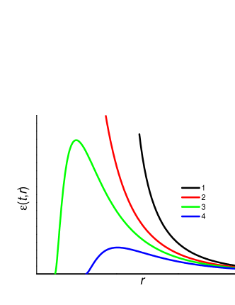
Figure 1: Energy density $\varepsilon(t,r)$ according to equation (35), $n=2$, for different times $t=t_{i}$ in the case of $kn<1$ (lines 1, 2: $t_{1}>t_{2}$) and $kn>1$ (lines 3, 4: $t_{3}<t_{4}$).

7 Summary and discussion

In this paper we considered relativistic potential flows of the perfect fluid that permit reductions to an equation for one scalar field. The restriction to the potential flow allowed us to derive analytic RHD solutions that are interesting from theoretical viewpoint, e.g., in the theory of elementary particle multiple production; they may be used to test numerical RHD computer routines. The relation between RHD and the scalar field proved to be most fruitful in the case of the extremely stiff EOS. In this case the problem is reduced to the linear wave equation for the scalar field yielding hydrodynamical solutions in the cases of planar, cylindrical and spherical symmetry. Moreover, a family of “non-symmetric” RHD solutions may be generated using multipole expansion for the scalar field; this is illustrated by examples that arise from combination of lower multipoles. We also found a family of nonlinear EOSs that permit analytic solutions defined inside the light cone and having behavior like that of famous scaling solutions [6, 7, 8, 9]. In the case of the linear EOS $p=\kappa\varepsilon$ some of our solutions reduce to these solutions [6, 7, 8, 9]. Also, we derived the solutions outside the light cone from self-similar solutions of the nonlinear scalar field equation.

Most of our solutions have light cone singularities like that of [6, 7, 8, 9]. These solutions cannot be directly matched with vacuum and may be used to describe a flow in a finite volume until it is destroyed by perturbations moving from the boundaries. Nevertheless, there are exceptions when regular solutions in a whole space may be generated, especially in the case of $k=1$ and in the case of spherical solutions (35) with $k>1/2$.

After we have sent the first version of our manuscript to the journal the paper [11] was published containing new interesting RHD solutions. Some of the solutions obtained in the present paper were independently found in [11] using different methods. In particular, our solution (35) corresponds to equations (24), (25) of [11] that have been obtained as an extension of “accelerating” solutions of [10]. Also, our solution (10) in the case of the plane flow and extremely stiff EOS is the same as solution (114), (115) of [11].

To outline possible generalizations, we note that the condition about the speed of sound ($0<k<1$ in the case of the linear EOS or equation (29) of Section 5) may be relaxed. This may be of some physical interest: the EOS with negative pressure, negative $k<0$ or $k>1$ are discussed in cosmology [19, 20], see also [25] concerning the possibility of “superluminal” EOS. The results of the Section 5 will be extended, if we do not restrict ourselves to simplest EOS in terms of elementary functions. In Section 6 we confine ourselves to the self-similar solutions of the field equation (34) of the form $\varphi=\varphi(r/t)$ thus yielding an ordinary differential equation. However, more general substitution $\varphi=r^{\alpha}\psi(r/t)$ also leads to an ordinary differential equation, though more complicated.

Appendix A Matching of solutions with vacuum

To perform this matching in a hydrodynamical way we use the condition of zero energy-momentum flux through a boundary with vacuum

$$T_{\mu}^{\nu}k_{\nu}=0,$$ (36)

where the vector $k_{\nu}$ is orthogonal to the boundary hypersurface. This yields

$$T_{\mu\nu}k^{\nu}=\varphi_{,\mu}\varphi_{,\nu}k^{\nu}-\frac{1}{2}k_{\mu}\left({\varphi_{,\alpha}\varphi_{,}^{\alpha}}\right)=0.$$

Simple analysis shows that this is possible only if at the boundary

$$\varphi_{,\alpha}\varphi_{,}^{\alpha}=0,\qquad\varphi_{,\alpha}k^{\alpha}=0.$$

In the two-dimensional case we have $\varphi_{,0}^{2}=\varphi_{,1}^{2}$.

Consider the light-like surface $t-r-t_{1}=0$, $\alpha=t_{1}$, then $k^{0}=k^{1}=-k_{1}=1$. In the case of the solution (11) the boundary condition is

$$T_{\mu\nu}k^{\nu}=\frac{\psi^{2}\left(\alpha\right)}{2r^{4}}k^{\mu},$$

that is at the boundary with vacuum $\psi\left({t_{1}}\right)=0$.

Acknowledgements

We are thankful to the referees of our paper for helpful remarks and suggestions. This work has been supported in part by “Cosmomicrophysica” program of National Academy of Sciences of Ukraine.

References

- [1]
- [2] Landau L.D., On the multiple production of particles in fast particle collisions, Izv. AN SSSR Ser. Fiz. 17 (1953), 51–64 (in Russian).
- [3] Khalatnikov I.M., Some questions of the relativistic hydrodynamics, J. Exp. Theor. Phys. 27 (1954), 529–541 (in Russian).
- [4] Landau L.D., Liftshitz E.M., Hydrodynamics, Nauka, Moscow, 1986 (in Russian).
- [5] Milekhin G.A., Nonlinear scalar fields and multiple particle production, Izv. AN SSSR Ser. Fiz. 26 (1962), 635–641 (in Russian).
- [6] Hwa R.C., Statistical description of hadron constituents as a basis for the fluid model of high-energy collisions, Phys. Rev. D 10 (1974), 2260–2268.
- [7] Cooper F., Frye G., Shonberg E., Landau’s hydrodynamical model of particle production and electron-positron annihilation into hadrons, Phys. Rev. D 11 (1975), 192–213.
- [8] Chiu C.B., Sudarshan E.C.G., Wang K.-H., Hydrodynamical expansion with frame-independence symmetry in high-energy multiparticle production, Phys. Rev. D 12 (1975), 902–908.
- [9] Bjorken J.D., Highly relativistic nucleus-nucleus collisions: the central rapidity region, Phys. Rev. D 27 (1983), 140–151.
- [10] Csörgö T., Nagy M.I., Csanád M., New family of simple solutions of relativistic perfect fluid hydrodynamics, nucl-th/0605070.
- [11] Nagy M.I., Csörgö T., Csanád M., Detailed description of accelerating, simple solutions of relativistic perfect fluid hydrodynamics, arXiv:0709.3677.
- [12] Pratt S., A co-moving coordinate system for relativistic hydrodynamics, Phys. Rev. C 75 (2007), 024907, 14 pages, nucl-th/0612010.
- [13] Blandford R.D., McKee C.F., Fluid dynamics of relativistic blast waves, Phys. Fluids 19 (1975), 1130–1138.
- [14] Pan M., Sari R., Self-similar solutions for relativistic shocks emerging from stars with polytropic envelopes, Astrophys. Journ. 643 (2006), 416–422, astro-ph/0505176.
- [15] Zhdanov V.I., Borshch M.S., Ultra-relativistic expansion of ideal fluid with linear equation of state, J. Phys. Stud. 9 (2005), 233–237, hep-ph/0508220.
- [16] Korkina M.P., Martynenko V.G., Homogeneous symmetric model with extremely stiff equation of state, Ukraiïn. Fiz. Zh. 21 (1976), 1191–1196 (in Russian).
- [17] Scherrer R.J., Purely kinetic -essence as unified dark matter, Phys. Rev. Lett. 93 (2004), 011301, 5 pages, astro-ph/0402316.
- [18] Chimento L.P., Lazkoz R., Atypical -essence cosmologies, Phys. Rev. D 71 (2005), 023505, 16 pages, astro-ph/0404494.
- [19] Sahni V., Dark matter and dark energy, Lect. Notes Phys. 653 (2005), 141–180, astro-ph/0403324.
- [20] Copeland E.J., Sami M., Tsujikawa S., Dynamics of dark energy, Internat. J. Modern Phys. D 15 (2006), 1753–1936, hep-th/0603057.
- [21] Lichnerowicz A., Relativistic hydrodynamics and magnetodynamics, Benjamin, New York, 1967.
- [22] Gorenstein M.I., Zhdanov V.I., Sinyukov Yu.M., On scale-invariant solutions in the hydrodynamical theory of multiparticle production, J. Exp. Theor. Phys. 74 (1978), 833–845 (in Russian).
- [23] Gorenstein M.I., Sinyukov Yu.M., Zhdanov V.I., On scaling solutions in the hydrodynamical theory of multiparticle production, Phys. Lett. B 71 (1977), 199–202.
- [24] Grigoriev S.B., Korkina M.P., Nonlinear scalar fields and Friedmann models, in Gravitation and Electromagnetism, Editor F.I. Fedorov, Izd-vo Universitetskoje, Minsk, 1987, 14–21 (in Russian).
- [25] Babichev E., Mukhanov V., Vikman A., -essence, superluminal propagation, causality and emergent geometry, arXiv:0708.0561.