A template bank to search for gravitational waves from inspiralling compact binaries: II. Phenomenological model

Abstract

Matched filtering is used to search for gravitational waves emitted by inspiralling compact binaries in data from ground-based interferometers. One of the key aspects of the detection process is the deployment of a set of templates, also called a template bank, to cover the astrophysically interesting region of the parameter space. In a companion paper, we described the template-bank algorithm used in the analysis of LIGO data to search for signals from non-spinning binaries made of neutron star and/or stellar-mass black holes; this template bank is based upon physical template families.

In this paper, we describe the phenomenological template bank that was used to search for gravitational waves from non-spinning black hole binaries (from stellar mass formation) in the second, third and fourth LIGO science runs. We briefly explain the design of the bank, whose templates are based on a phenomenological detection template family. We show that this template bank gives matches greater than 95% with the physical template families that are expected to be captured by the phenomenological templates.

I Motivation

The Laser Interferometer Gravitational-Wave Observatory (LIGO) detectors LIGO have reached their design sensitivity curves. The fifth science run (S5) began in November 2005 and should be completed by the end of 2007, with the goal of acquiring a year’s worth of data in coincidence between the three LIGO interferometers. Each successive LIGO science run has witnessed improvement from both experimental and data analyst’s point of view. On the experimental side, better stationarity of the data and detector sensitivities closer to design sensitivity curve were achieved. On the data analysis side, the search pipeline was tuned, and new techniques were developed to reduce the background rate while keeping detection efficiencies high.

Among the sources of gravitational waves that ground-based detectors are sensitive to, inspiralling compact binaries are among the most promising. Several searches for inspiralling compact binaries in the LIGO data have been pursued: primordial black holes (PBH) LIGOS2macho ; LIGOS3S4 , binary neutron stars (BNS) LIGOS1iul ; LIGOS2iul ; LIGOS3S4 , and intermediate mass binary black holes (BBH) LIGOS2bbh ; LIGOS3S4 . These searches used matched filtering technique, which is the most effective and commonly used method to search for inspiralling compact binaries.

Matched filtering computes cross correlation between the detector output and a template waveform. If the template waveform is identical to the signal then the method is optimal, in the sense of signal-to-noise ratio (SNR). However, in general, the template waveforms differ from the signals. Indeed, modelizations can only approximate the exact solution of the two-body problem. In addition, template waveforms are constructed with a subset of the signal’s parameters (e.g., the two component masses whereas eccentricity and spins effects may be neglected). In this work, we consider only the case of non-spinning waveforms so that the signals are entirely defined by 4 parameters: 2 mass components, the time of arrival and the initial phase. Because the signal’s parameters are unknown, the detector output must be cross correlated with a set of template waveforms, which is called a template bank. While the spacing between templates can be decreased most certainly, and this is the insurance of a SNR close to optimality, it also increases the size of the template bank (i.e., the computational cost). The distance between templates is governed by the trade-off between computational cost and loss in detection rate; therefore, template bank placement is a key aspect of the detection process.

In a companion paper squarebank , we proposed a template bank with a minimum match of 95%. We assume that both template and signal were based on the same physical template family (precisely, the stationary phase approximation with the phase described at 2PN order BDI95 ; droz1997 ). We have shown that the template bank could be used, effectively, to search for BNS, PBH, black hole - neutron star (BHNS), and BBH systems. In this paper, we consider the case of BBH systems only.

There is a wide variety of techniques used to describe the gravitational flux and energy generated during the late stage of the inspiralling phase (e.g., see LB ). However, they lead to various physical template families, and overlaps between them are not necessarily high. In the case of heaviest systems, post-Newtonian (PN) expansion LB begins to fail as the characteristic velocity $v/c$ is not close to zero anymore (e.g., see BCV ). In addition, even though heavier BBH systems are accessible each time the detector sensitivity improves in the low frequency range, BBH waveforms remain short in the LIGO band. For instance, during the second science run (S2) LIGOS2bbh , the lower cut-off frequency was set to 100 Hz, which restricted the total mass of the search to be below $40~{}M_{\odot}$, and the longest expected signal to last about 0.60 s.

There exist several template families, and there is no reason to select one in particular. A solution may be to filter the detector output with a set of template banks, each of them associated with a different physical template families. We have shown in hexabank that a unique template bank placement could be used effectively with several template families. However, we investigate only 4 different families at 2PN order. A different template bank might be necessary for other template families. More importantly, the number of template families could be large, and computational cost not manageable. Instead of searching for BBH signals using several physical template families, a single detection template family(DTF) was proposed by Buonanno, Chen, and Vallisneri BCV (BCV) with the goal of embedding the different physical approximations all into a single phenomenological model. This detection template family is known as BCV template family and has been used to search for non-spinning BBH signals in LIGO data LIGOS2bbh ; LIGOS3S4 .

In this paper, we do not intend to compare a search that uses BCV templates and a search based upon physical template family. Our main goal is to describe the BCV template bank that was developed and used to search for stellar-mass BBH signals in the second (S2), third (S3), and fourth (S4) LIGO science runs LIGOS2bbh ; LIGOS3S4 . In section II, we briefly discuss the template parameters and the filtering process related to BCV templates. In section III, we describe the BCV template bank, and the the spacing between templates. In section IV, we test and validate the proposed template bank with exhaustive simulated injections. Finally, in section V, we summarize the results.

II The BCV template family

The detection template family that was proposed in BCV is built directly from the Fourier transform BSD95 of gravitational-wave signals by writing the amplitude and phase as polynomials in the gravitational-wave frequency law that appear in the stationary phase approximation SD91 . In the frequency domain, the BCV templates are defined to be

$$h\left(f\right)=\mathcal{A}(f)e^{i\psi\left(f\right)}\,,$$ (1)

where

$$\mathcal{A}(f) = f^{-7/6}\left(1-\alpha f^{2/3}\right)\theta\left(f_{\rm cut}-f\right),\,$$ (2)

$$\psi(f) = 2\pi ft_{0}+\phi_{0}+f^{-5/3}\sum_{k=0}^{N}\psi_{k}f^{k/3}\,.$$ (3)

The parameters $t_{0}$ and $\phi_{0}$ are the standard time of arrival and initial phase of the gravitational wave signal. The parameter $\alpha$ is a shape parameter introduced to capture post-Newtonian amplitude corrections. Because various models predict different terminating frequencies, an ending cut-off frequency $f_{\rm cut}$ is introduced. In the amplitude expression, the waveform is multiplied by a Heaviside step function, $\theta\left(f_{\rm cut}-f\right)$. In the right hand side of equation 3, we use only two parameters $\psi_{0}$ and $\psi_{3}$, which suffices to obtain a high match with most of the PN models BCV . The symbol $\psi_{3}$ here is the same as the symbol $\psi_{3/2}$ in BCV .

The $\psi_{k}$ parameters are the phase parameters of the phenomenological waveform, which cannot be directly linked to the physical mass parameters; the BCV templates are made for detection, not for parameter estimation. Nevertheless, a good approximation (for low masses) of the chirp mass $\mathcal{M}$ is given by

$$\psi_{0}\approx\frac{3}{128}\left(\frac{1}{\pi\mathcal{M}}\right)^{5/3}\,.$$ (4)

In section IV.4, we investigate the range of validity of this relation.

The filtering of a data set using BCV templates is not as trivial as the one that uses physical template families. Indeed, the BCV filtering implies a search in six dimensions ($\psi_{0}$, $\psi_{3}$, $\alpha$, $\phi_{0}$, $t_{0}$, and $f_{\rm cut}$). The SNR can be analytically maximized over $\alpha$, $\phi_{0}$ and $t_{0}$, which reduces the search to three dimensions only. the maximization over $\alpha$ and $\phi_{0}$ is not. In order to perform the filtering and the maximization over $\alpha$ and $\phi_{0}$, we need to construct orthonormal basis vectors $\left\{\hat{h}_{k}\right\}_{k=1,..,4}$ for the 4-dimensional linear subspace of templates with $\phi_{0}\in\left[0,2\pi\right)$ and $\alpha\in\left(-\infty,\infty\right)$, and we want the basis vectors to satisfy $\left\langle\hat{h}_{i}\Big{|}\hat{h}_{j}\right\rangle=\delta_{ij}$ (see the Appendix for details). The SNR before maximization is given by

$$\rho = x_{1}\cos{\omega}\cos{\phi_{0}}+x_{2}\sin{\omega}\cos{\phi_{0}}$$

$$+ x_{3}\cos{\omega}\sin{\phi_{0}}+x_{1}\sin{\omega}\sin{\phi_{0}}\,,$$

where $x_{i}=\left\langle s\Big{|}\hat{h}_{i}\right\rangle$, and $s$ is the data to be filtered . The parameter $\omega$ is a function of $\alpha$ (see equation 14 and 15).

The SNR $\rho$ can be maximized over $\phi_{0}$ and $\omega$($\alpha)$. In LIGOS2bbh , the maximization is done over the two new parameters $A=\omega+\phi_{0}$ and $B=\omega-\phi_{0}$. The maximized SNR (independent of $\alpha$ and $\phi_{0}$), is denoted $\rho_{U}$, and is given by

$$\rho_{U}=\frac{1}{\sqrt{2}}\left(\sqrt{V_{0}+\sqrt{V_{1}^{2}+V_{2}^{2}}}\right)\,,$$ (6)

where $V_{k}$ are function of $x_{i}$ (see Appendix and equations 19, 20 and 20).

The SNR provided in equation 6 is the unconstrained SNR that is independent of any constraint on the range of the parameter $\alpha_{F}^{U}=\alpha f^{2/3}$ (again, here the index $U$ represents the unconstrained case, and we shall use $C$ for the constrained case). Yet, in BCV , the authors suggested that the parameter $\alpha_{F}^{U}$ should be restricted to the range $[0,1]$. Indeed when $\alpha_{F}^{U}>1$, the amplitude in equation 2 becomes negative, which corresponds to unphysical waveforms. Moreover, when $\alpha_{F}^{U}<0$, the amplitude factor can substantially deviate from the predictions of PN theory.

In S2 LIGOS2bbh , many accidental triggers were found with $\alpha_{F}^{U}>1$, and the calculation of the SNR was unconstrained (as in equation 6) leading to a high false alarm rate, which was decreased, a posteriori, by removing all triggers for which $\alpha_{F}^{U}>1$ (without decreasing the detection efficiency). Nevertheless, triggers that verified $\alpha_{F}^{U}<0$ were kept because the false alarm rate did not decrease significantly when this selection was applied.

In S3 and S4, the search for BBH systems deployed a filtering that takes $\alpha_{F}^{U}$ value into account, by using a maximization of equation II that leads to a constrained SNR denoted $\rho_{C}$. The expression for the constrained SNR depends now on the value of $\alpha_{F}^{U}$. We have $\alpha_{F}^{C}=\alpha_{F}^{U}$ if $0\leq\alpha_{F}^{U}\leq 1$, and no constraint is applied (i.e., $\rho_{C}=\rho_{U}$). However, if $\alpha_{F}^{U}<0$ or $\alpha_{F}^{U}>1$, then a constrained SNR is used so that the final $\alpha_{F}^{C}$ parameter is 0 and 1, respectively, and $\rho_{C}\leq\rho_{U}$. The expressions of the constrained SNR are provided in the Appendix.

Let us make the point clear. In the contrained-SNR case, as explained above, $\alpha_{F}^{C}=\alpha_{F}^{U}$ if $0<\alpha_{F}^{U}<1$ only. Otherwise $\alpha_{F}$ takes only two values (0 or 1) but we know $\alpha_{F}^{U}$ (since it is the condition to apply the constraint or not).

It is worth noticing that for the study that follows, we always use a constrained SNR but using an unconstrained SNR should not significantly change the results of our simulations and/or template bank placement. Indeed, simulated injections are generated with physical template families for which we do not expect $\alpha_{F}$ to be unphysical (i.e., outside $[0-1]$), as we shall see in section V. Using a constrained SNR has an important impact when dealing with real analysis, where most of the accidental triggers have $\alpha_{F}$ between $\ \left(-\infty\,,\infty\right)$ (and therefore in $(-\infty\,,0[\;\cup\;]1\,,\infty)$ as well, where $\rho_{C}<\rho_{U}$). Consequently, in general, for a given threshold $\lambda$, the SNR of accidental triggers have $\rho_{C}<\rho_{U}$, and the rate is therefore lower with respect to a search with unconstrained SNR. The number of triggers that needs to be stored is lower by an order of magnitude. Nevertheless, the final rate of triggers between the two methods may be equivalent because of a posteriori cuts on $\alpha_{F}$ when an unconstrained SNR is used as in LIGOS2bbh .

III BCV template bank design

Template bank placement has been investigated in several papers Owen96 ; OwenSathyaprakash98 ; buskulic ; squarebank ; hexabank ; flatbank in the context of physical template families. We refer the reader to the established literature in this subject area.

III.1 Metric Computation in $\psi_{0}\textrm{--}\psi_{3}$ Plane

In the case of BCV templates, the mismatch metric $g_{ij}$ Owen96 is known (see Appendix), and is constant over the entire $\psi_{0}\textrm{--}\psi_{3}$ parameter space. Nonetheless, the metric components are strongly related to the lower cut-off frequency of the search, which affects the moments used to calculate the metric (see equation 38). The moment computation also depends on the $\alpha$ parameter, as discussed later. For now, let us suppose that the moments are fixed.

Because the metric is constant, the placement of templates on the $\psi_{0}\textrm{--}\psi_{3}$ parameter space is straightforward. In the first search for BBH signals LIGOS2bbh , the template placement used a square lattice, and templates were placed parallel to the $\psi_{0}$ axes. In S3 and S4 BBH searches, an optimal placement was used (hexagonal lattice), which reduced the requested computing resources (and trigger rate) by 30% with respect to S2. In this paper, we only consider tests related to the hexagonal lattice case. In S3 and S4 BBH searches, we placed the templates parallel to the first eigenvector rather than parallel to the $\psi_{0}$ axis.

The target waveforms are BBH systems for which the lowest component mass is set to $3~{}M_{\odot}$ and the highest component mass is defined by the detector lower cut-off frequency (up to $80~{}M_{\odot}$ in S4). Simulations show that to detect such target waveforms, the range of phenomenological parameters should be set to $\psi_{0}\in[10000,\;550000]~{}{\rm Hz}^{5/3}$ and $\psi_{3}\in[-5000,\;-10]~{}{\rm Hz}^{2/3}$. As explained in section III.4, if we search for BBH systems only, a significant fraction of those templates are not needed and can be removed from the template bank.

III.2 $\alpha_{B}$-dependence

The moments used to estimate the metric components strongly depend on the parameter $\alpha$. We refer to this parameter as $\alpha_{B}$ to differentiate from the $\alpha$ parameter (or equivalently from $\alpha_{F}$) that is used in the filtering process. As shown in figure 1, the number of templates changes significantly when $\alpha_{B}$ varies. There is a drop in the number of templates around $\alpha_{B}=10^{-2}$. We want to minimize the template bank size but we also need to consider the efficiency of the bank as defined in squarebank ; hexabank , and choose $\alpha_{B}$ appropriately. Indeed, we expect the efficiency of the template bank to be also affected by this parameter. We performed simulated injections so as to test the efficiency of the template bank for various values of $\alpha_{B}$. Results are summarized in figure 2 for three typical values of $\alpha_{B}$. Because efficiencies are very similar, we decided to use an $\alpha_{B}$ parameter such that the number of templates is close to a minimum, that is $10^{-2}$. In all the following simulations and LIGO searches, $\alpha_{B}=10^{-2}$.

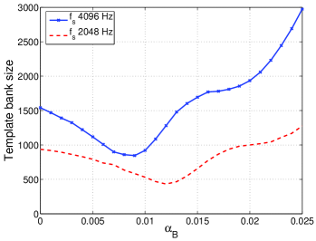
Figure 1: The size of the template bank function of the $\alpha_{B}$ parameter. The two curves show the template bank size versus $\alpha_{B}$ parameter for two values of sampling frequency. The two curves show the same pattern with a drop around $\alpha_{B}=10^{-2}$, where template bank sizes are twice as low as compared to $\alpha_{B}=0$ or $\alpha_{B}=2.5\times\,10^{-2}$. This evolution of the template bank size is directly linked to the moment computation (see equation 38), where the parameter $\alpha_{B}$ is used. Efficiency of a template bank is not strongly related to this parameter (see figure 2) so we choose a value that corresponds to the smallest bank size. In real analysis, we use 2048 Hz and for simplicity a value of $\alpha_{B}=10^{-2}$ was chosen. In this example, we used the same simulation parameters as in section IV.1.

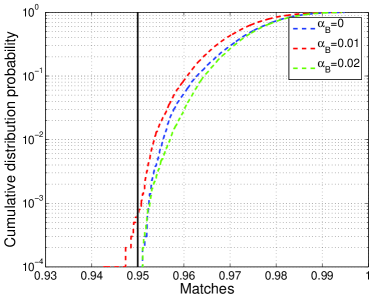
Figure 2: Template bank efficiencies versus $\alpha_{B}$ parameter. The $\alpha_{B}$ parameter does not significantly affect the matches. Most of them are above the minimal match of 95%, and more importantly the three distributions are close to each other. In this example, we used the same simulation parameters as in section IV.1, and EOB injections.

III.3 Template Bank using ending frequency layers

Starting from each template that is placed in the $\psi_{0}\textrm{--}\psi_{3}$ plane, we need to lay templates along the third dimension, which is the ending cut-off frequency $f_{\rm cut}$ of the template. Because the mismatch is first order in $\Delta f_{\rm cut}$ BCV , it cannot be described by a metric.

Using an exact formula, BCV proposed to lay templates with different $f_{\rm cut}$ values between $f_{\rm min}$ and $f_{\rm end}=f_{\rm Nyquist}$ that depend on the region searched for. We populate the $f_{\rm cut}$ dimension as follows. First, we estimate the frequency of the last stable orbit which we refer to as $f_{\rm min}$, and the frequency at the light ring which we refer to as $f_{\rm max}$. Between $f_{\rm min}$ and $f_{\rm max}$, we place $N_{\rm cut}$ layers of templates with the ending frequency chosen at equal distance between $f_{\rm min}$ and $f_{\rm max}$. The frequency at the last stable orbit and light ring are defined in terms of the total mass ($f_{\rm min}=1/(M\pi 6^{3/2})$, $f_{\rm max}=1(M\pi 3^{3/2})$). The total mass is computed for each template using an empirical expression similar to equation 4: $M\approx-\psi_{3}/(32\pi^{2}\psi_{0})$. This expression is an approximation. It underestimates the total mass for low mass range, however, it is suitable for the wide range of mass that we are interested in: the final template bank gives high match with the various physical template families, as shown in section IV. In all our simulations and searches, we set the minimal match $(MM)$ Owen96 to $95\%$, so there is no guarantee that the relation between $M$ and $\psi_{0,3}$ is suitable for minimal matches far from 95%.

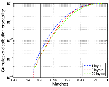
Figure 3: Template bank efficiencies versus number of layers, $N_{\rm cut}$ , in the $f_{\rm cut}$ dimension. With the current template bank design, $N_{\rm cut}$ does not affect the matches significantly. The cumulative distribution of matches over 10,000 simulations shows only small differences between 3 and 20 layers. Even the results obtained with 1 layer are not that far from $N_{\rm cut}=3$. In our real analysis and simulations, we used $N_{\rm cut}=3$. In this example, we used the same simulation parameters as in section IV.1, and EOB simulated injections.

III.4 Polygon Fit

The boundaries of the template bank are defined by the ranges of the parameters $\psi_{i}$ and the span of the cut-off frequency $f_{\rm cut}$ in such a way that BBH systems with component mass as low as $3~{}M_{\odot}$ are detectable. The $\psi_{i}$ ranges provided in section III.1 cover a squared area that is actually too wide: a significant fraction of the templates are not targeting the BBH systems we are searching for. Therefore, in order to reduce the template bank size and optimize our searches, we introduce an extra procedure that selects the pertinent templates only. This procedure is known as a polygon fit and works as follows. First, we create a BCV template bank with the range of $\psi_{0}$ and $\psi_{3}$ parameters as large as possible, and for our purpose, as quoted in section III.1. This choice of ranges allows us to not only detect BBH systems but also BHNS systems. Since, we focus on the BBH systems only, we perform many BBH simulated injections and filter them with the template bank that has been created. For each injection, we keep the $\psi_{0}$ and $\psi_{3}$ parameters of the template that gives the best match. We gather all the final pairs of $\psi_{0}$, $\psi_{3}$ parameters, and superpose them on top of the original template bank. It appears that only about a third of the templates are required to detect BBH systems with a high match. This sub-set of templates can be used to define a polygon area that enclose all of them. The resulting polygon area defines the boundaries of our new template bank and results in a template bank three times smaller than the original one.

In figure 4, we show such a template bank that is within the boundary of a polygon constructed with our simulated injections. The coordinates of this polygon are chosen empirically. For safety, the boundaries are chosen loosely, therefore the template bank has also the ability to detect non-spinning BHNS. It is worth noticing that with this template bank designed to detect BBH many BHNS systems are found with a match greater than the requested $MM$ (See section IV.3).

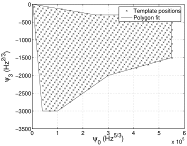
Figure 4: Example of parameter space and template bank placement. This plot shows a projection of the templates onto the $\psi_{0}/\psi_{3}$ plane. Simulations and equation 4 gives an estimation of the mapping between the phenomenological parameters and the chirp mass of the simulated injections. Low mass systems such as a $(3,3)M_{\odot}$ are in the RHS, high mass systems lie on the LHS and asymmetric systems in the bottom left corner. In this example, we used the same parameters as in section IV.2.

IV Simulations

In the following simulations, we fix the sampling frequency to $2048$ Hz, $\alpha_{B}=10^{-2}$, $N_{\rm cut}=3$, the $\psi_{0}$ and $\psi_{3}$ ranges are provided in section III.1 and a polygon fit as in figure 4 is used. The simulated injections are based on several physical template families that are labelled EOB, PadeT1, TaylorT1, and TaylorT3 EOB1 ; EOB2 ; EOB3 ; Standard ; DIS with the phase expressed at 2PN order (see hexabank for more details). The population of simulated injections has a uniform total mass. Although this choice is not based on any astronomical observation, it is convenient to estimate the efficiency of our template banks. We use a noise model that mimics the design sensitivity curve of initial LIGO (see hexabank ; BSD95 ), and the minimal match is $MM=95\%$. We performed 2 simulations that are closely related to the third and fourth LIGO science run’s BBH searches LIGOS3S4 .

IV.1 Example 1

The first set of simulations uses a lower cut-off frequency of $70$ Hz, as in S3 BBH search LIGOS3S4 . The maximal total mass of the simulated injections is set to $40~{}M_{\odot}$ and therefore the largest component mass to $37~{}M_{\odot}$. The template bank has 531 templates. The results are summarized in figure 5 which shows the efficiency of the template bank versus the total mass. There are a few injections found with a match as low as 93% for total mass $M<6.5~{}M_{\odot}$. Closer inspection shows that several issues are linked to this feature. First, we used a sampling frequency of 2048 Hz, which reduces the template bank size by $\approx 50\%$ as compared to a sampling of 4096 Hz. Second, we set $\alpha_{B}=10^{-2}$, which reduces the template bank size by $\approx 50\%$ as compared to $\alpha_{B}=0$. Finally, the number of layers, $N_{\rm cut}$, is limited to 3. Therefore, this tuning significantly reduced the template bank size with the cost of losing about only 1 to 2% SNR for a small fraction of the parameter space considered. From $M=6.5~{}M_{\odot}$ to about $M=20~{}M_{\odot}$, matches are above 95%. In the high mass range, a large fraction of the simulated injections are found below the minimal match (but larger than 90%): 20% in the case of TaylorT1, TaylorT3, and PadeT1 models, and only 0.1% in the case of EOB injections. This effect is expected because the lower cut-off frequency is high, and therefore many of the high mass systems considered are very short (i.e., less than 100 ms). Because the final frequency of the EOB signals goes up to the light ring, the matches are larger than in the case of TaylorT1, TaylorT3, and PadeT1 approximants, whose last frequencies stop at the last stable orbit.

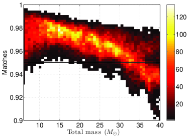
Figure 5: Distribution of the efficiency versus the total mass. The simulation consisted of $N_{s}=40,000$ injections. The lower cut-off frequency for the injections and the BCV templates was set to 70 Hz, as in S3 BBH search.

IV.2 Example 2

The second set of simulations uses a lower cut-off frequency of $50$ Hz, as in S4 BBH search LIGOS3S4 . The maximal total mass of the simulated injections is set to $80~{}M_{\odot}$ and therefore the largest component mass to $77~{}M_{\odot}$. The template bank has 1609 templates. The results are summarized in figure 6. Up to $M\approx 40~{}M_{\odot}$, most of the injected simulations are recovered with matches above 95%. However, a small fraction is found with matches below 95%, which represent 0.1% of the EOB, PadeT1, and TaylorT1 injections, and 3% of the TaylorT3 injections. In the high mass region (up to $60~{}M_{\odot}$), 20% of the injections are below the required minimal match for the TaylorT1, TaylorT3, and PadeT1 injections, and only 0.5% of the EOB injections. If we consider injections with total mass from 60 to $80~{}M_{\odot}$, almost 10% of EOB are below the minimal match (but above 92%). As for other models, matches drop quickly towards zero down to 40%, which is due to shorter and shorter duration of the injected waveforms.

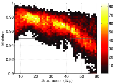
Figure 6: Distribution of the efficiency versus the total mass. The simulation consisted in $N_{s}=40,000$ injections. The lower cut-off frequency of the injections and the BCV templates is 50 Hz, as in S4 BBH search. For convenience (same scale as in figure 5), we do not show simulated injections with total mass above $60~{}M_{\odot}$ and matches below 90% (see text for details).

IV.3 Example 3

As stated in section III.4, although the template bank is designed to target BBH systems, it has the ability to detect some BHNS systems as well. The goal of this third simulation is to demonstrate that indeed many BHNS systems are detectable with a high match by using the template designed to search for BBH systems in S3 and S4 data sets.

The parameters used are exactly the same as in the second example. The maximal total mass of the simulated injections is set to $80~{}M_{\odot}$, the largest component to $79~{}M_{\odot}$, and the lowest component mass is set to $1~{}M_{\odot}$. We impose the systems to be BHNS only (the mass of the neutron star is less than $3~{}M_{\odot}$, and the mass of the black hole is larger than $3~{}M_{\odot}$). The template bank is identical to the second simulation (1609 templates). The results are summarized in figure 7, where we plot matches as a function of the two component masses. We found that 60% of the BHNS injections are recovered with the match larger than 95%, 77% with the match larger than 90%, and 98% with the match greater than 50%. Therefore, using the same bank as in S3 and S4 searches, whose boundaries resulting from the polygon fit were deliberately chosen to be slightly wider than necessary, we can detect a significant fraction of the BHNS systems. It is also clear from the figure that the lightest systems have a very low match. This was expected since the template bank aimed at detecting systems whose total mass is greater than $6M_{\odot}$, as defined by the maximum of the $\psi_{0}$ range.

We performed a second test where the polygon fit is not applied anymore. The template bank is then much larger with 4635 templates but we found that 78% of the BHNS injections are recovered with a match larger than 95%, 94% with a match larger than 90%, and 98% with a match greater than 50%. The size of such a template bank is comparable to a template bank that uses physical template families (e.g., with the same parameters as above, a hexagonal placement for physical template families hexabank that covers a parameter space from 1 to 80 solar mass has about 3000 templates if we exclude the templates for which both component mass are below 3 $M_{\odot}$).

The events which are found with a low match (say, 60% or lower) correspond to low mass systems where the neutron star’s mass is less than $2.5~{}M_{\odot}$ and the BH’s mass less than $7~{}M_{\odot}$ which can be taken care of by increasing the range of $\psi_{0}$.

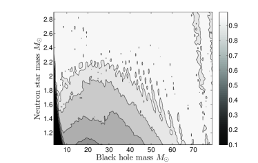
Figure 7: Matches between the BCV template bank used to search for BBH systems and BHNS injections. The simulation consisted in $N_{s}=100,000$ injections. We found that 77% of the BHNS injections have a match larger than 90%. See the text for more details.

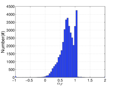
Figure 8: Distribution of the $\alpha_{F}^{U}$ parameter corresponding to simulations made in section IV.2. Most of the found simulated injections have an $\alpha_{F}^{U}$ value between zero and unity. However, a significant fraction are distributed around $\alpha_{F}^{U}=1$. Those triggers correspond to $M>60~{}M_{\odot}$, for which waveforms cannot be differentiated from a transient noise (short duration).

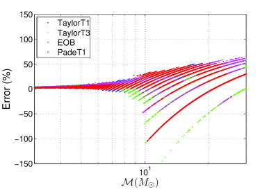
Figure 9: Errors in chirp mass estimation corresponding to simulations made in section IV.2. Errors increase significantly for $\mathcal{M}$ greater than 8 solar mass with errors larger than 50%.

IV.4 Discussions

In this section, we use the results of section IV.2 to check (i) the range of validity of equation 4, which gives an estimation of the chirp mass, and (ii) the regime of constrained SNR (i.e., the value of $\alpha_{F}$).

Although we use a constrained SNR, we kept track of the value of $\alpha_{F}^{U}$ before the maximization. We plot the distribution of $\alpha_{F}^{U}$ in figure 8. About 83% of the injections were found with a $\alpha_{F}^{U}$ value in the range ]0,1[. Therefore, as stated in section II, the results obtained with the constrained SNR are very similar to what we would have obtained if we had used the unconstrained SNR. The distribution has a first peak around 0.7 and a second peak in the range [1, 1.1], which correspond to about 15% of the injections; it corresponds to total mass above $60~{}M_{\odot}$.

In figure 9, we plot the errors on the chirp mass (i.e., $(\mathcal{M}_{i}-\mathcal{M}_{e})/\mathcal{M}_{i}$, where $i$ stands for injected, and $e$ for estimated). We used equation 4 to estimate the chirp mass. The errors are within 10% for BBH systems when the chirp mass is below $\approx 8~{}M_{\odot}$. However, errors increase significantly when $\mathcal{M}\gtrsim 8~{}M_{\odot}$ because (i) parameter estimation of high mass BBH systems is intrinsically weak, even for physical template families and (ii) BCV templates are known to be detection template families that are not suitable for parameter estimation.

V Conclusions

The BCV template bank that we described in this paper was used to search for BBH systems in the S2, S3 and S4 LIGO data sets. We described the significant improvements that were made between the S2 search and the S3/S4 searches: $\alpha_{B}$ tuning, hexagonal lattice, and polygon fit. These improvements reduce the template bank size by an order of magnitude, while keeping the efficiency higher than 95% for most of the BBH systems considered. Consequently, despite reducing the lower cut-off frequency from 100Hz to 50Hz between the second and the fourth science runs, the template bank size remained similar.

A principal motivation for the construction of a detection template bank was to use a single template bank instead of several physical template families. The template bank size is therefore an important aspect of a BCV search, and we have shown in this work how the number of templates can be optimized to search for BBH. Remarkably, the same template bank has a high match with a wide range of BHNS.

More importantly, the BCV template bank was designed to search for BBH systems in the context of the S2 LIGO search. That is, for a lower cut-off frequency of 100 Hz for which most of the target waveforms are short duration waveforms. However, LIGO detectors improved and are still improving at low frequency, making the waveforms longer. The advantage of using a BCV template to search for systems as low as $3~{}M_{\odot}$ is no longer evident, especially considering the absence of a well defined $\chi^{2}$ test for phenomenological templates. Therefore if it were to be used, the author thinks that a BCV template bank should be used to search for a mass range starting at a higher value, such as $10$ or $20~{}M_{\odot}$.

Appendix A Filtering, $\alpha$-maximization, and constrained SNR

We define the inner product as follows

$$\left<h_{1}\Big{|}h_{2}\right>=4Re\left(\int_{0}^{\infty}\frac{h_{1}(f)h_{2}^{*}(f)}{S_{h}(f)}df\right)\,,$$ (7)

where $S_{h}(f)$ is the one-sided noise power spectral density.

A.1 Filtering

The BCV templates in the frequency domain are defined by equation 1. The amplitude part of a BCV template $\mathcal{A}(f)$ can be decomposed into linear combinations of $f^{-7/6}$ and $f^{-1/2}$. These expressions can be used to construct an orthonormal basis $\{\hat{h}_{k}\}_{k=1..4}$. We want the basis vectors to satisfy

$$\left<\hat{h}_{i}\Big{|}\hat{h}_{j}\right>=\delta_{ij}.$$ (8)

First, we construct two real functions $\mathcal{A}_{1}(f)$ and $\mathcal{A}_{2}(f)$ that satisfy $\left<A_{i}\big{|}A_{j}\right>=\delta_{ij}$. Then, we define $\hat{h}_{1,2}(f)=\mathcal{A}_{1,2}(f)e^{i(\psi-\phi_{0})},\hat{h}_{3,4}(f)=i\mathcal{A}_{1,2}(f)e^{i(\psi-\phi_{0})}$ which will give $\left<\hat{h}_{i}\big{|}\hat{h}_{j}\right>=\delta_{ij}$, and the desired basis, $\{\hat{h}_{k}\}$. $\psi$ is the phase of the signal, as defined in equation 3, and $\phi_{0}$ the initial phase that we want to maximize. We can choose the following basis functions

$$\left[\begin{array}[]{cc}\mathcal{A}_{1}(f)\\ \mathcal{A}_{2}(f)\end{array}\right]=\left[\begin{array}[]{cc}a_{11}&0\\ a_{21}&a_{22}\end{array}\right]\left[\begin{array}[]{cc}f^{-7/6}\\ f^{-1/2}\end{array}\right],$$ (9)

where the normalization factor are given by

$$a_{11}=I^{-1/2}_{7/3},a_{21}=-\frac{I_{5/3}}{I_{7/3}}\left(I_{1}-\frac{I^{2}_{5/3}}{I_{7/3}}\right)^{-1/2},$$ (10)

$${\rm and\;}a_{22}=\left(I_{1}-\frac{I^{2}_{5/3}}{I_{7/3}}\right)^{-1/2}\,,$$ (11)

and the integrals $I_{k}$ are defined by

$$I_{k}=4\int_{0}^{f_{\rm cut}}\frac{f^{-k}}{S_{h}(f)}df.$$ (12)

The normalized template can be parametrized using the orbital phase $\phi_{0}$ and an angle $\omega$

$$\hat{h}(\theta,\omega;f) =$$

$$\hat{h}_{1}(f)\cos\omega\cos\phi_{0}+\hat{h}_{2}(f)\sin\omega\cos\phi_{0}$$

$$+ \hat{h}_{3}(f)\cos\omega\sin\phi_{0}+\hat{h}_{4}(f)\sin\omega\sin\phi_{0}$$

where $w$ is related to $\alpha$ by (see LIGOS2bbh )

$$\tan{\omega}=-\frac{a_{11}\alpha}{a_{22}+a_{21}\alpha}\,,$$ (14)

which can be inverted to get $\alpha$

$$\alpha=-\frac{a_{22}\tan{\omega}}{a_{21}\tan{\omega}+a_{11}}.$$ (15)

It follows that for any given signal $s$, the overlap is

$$\rho = \left<s\Big{|}\hat{h}\right>$$

$$= x_{1}\cos\omega\cos\phi_{0}+x_{2}\sin\omega\cos\phi_{0}$$

$$+ x_{3}\cos\omega\sin\phi_{0}+x_{4}\sin\omega\sin\phi_{0},\,$$

where $x_{i}=\left<s\Big{|}\hat{h}_{i}\right>$. We can then maximized over $\omega$ (i.e., $\alpha)$, and $\phi_{0}$ without any constraint on the $\alpha$ parameter, which leads to the unconstrained SNR given by

$$\rho_{U}=\frac{1}{\sqrt{2}}\sqrt{\left(V_{0}+\sqrt{V_{1}^{2}+V_{2}^{2}}\right)}$$ (17)

where

$$V_{0} = x_{1}^{2}+x_{2}^{2}+x_{3}^{2}+x_{4}^{2}\,,$$ (18)

$$V_{1} = x_{1}^{2}+x_{3}^{2}-x_{2}^{2}-x_{4}^{2}\,,$$ (19)

$$V_{2} = 2(x_{1}x_{2}+x_{3}x_{4}).$$ (20)

The values of $\omega$ and $\phi_{0}$ that maximize $\rho_{U}$ are provided in LIGOS2bbh as function of the $x_{i}$. We reformulate $\omega^{\rm max}$ using the $V_{i}$ and found this simple expression:

$$\tan{2\omega^{\rm max}}=\frac{V_{2}}{V_{1}}\,.$$ (21)

It is then straightforward to obtain $\alpha^{\rm max}$ using equation 15, and $\alpha_{F}^{U}=\alpha^{\rm max}f^{2/3}$.

A.2 constrained and unconstrained SNRs

Starting from equation A.1, we can derive a constrained SNR $\rho_{C}$ that depends upon the value of the parameter $\alpha_{F}$. Therefore, we need to maximize equation A.1 over the parameter $\phi_{0}$ only. This maximization gives

$$\rho(\omega)=\max_{\omega}\frac{1}{\sqrt{2}}\sqrt{V_{0}+V_{1}\cos 2\omega+V_{2}\sin 2\omega}\,.$$ (22)

If $\alpha_{F}<0$, we want to use a SNR calculation for which $\omega=0$, which means $\alpha_{F}^{C}=\alpha=0$. Therefore, the constrained SNR is

$$\rho_{C}^{0}=\frac{1}{\sqrt{2}}\sqrt{V_{0}+V_{1}}\,.$$ (23)

If $\alpha_{F}>1$, we want to use a SNR calculation for which $\omega=\omega_{\rm max}$, which means that $\alpha_{F}^{C}=1$ (i.e., $\alpha=f_{\rm cut}^{-2/3}$). Using equation 14, the angle $\omega=\omega_{\rm max}$ is then a maximum given by

$$\omega_{\rm max}=\arctan\left\{-\frac{a_{1}f_{\rm cut}^{-2/3}}{b_{2}+b_{1}f_{\rm cut}^{-2/3}}\right\}.$$ (24)

The constrained SNR is then given by

$$\rho_{C}^{1}=\frac{1}{\sqrt{2}}\sqrt{V_{0}+V_{1}\cos 2\omega_{\rm max}+V_{2}\sin 2\omega_{\rm max}}\,.$$ (25)

Finally, using the relation $V_{1}\cos 2\omega+V_{2}\sin 2\omega=\sqrt{V_{1}^{2}+V_{2}^{2}}\cos{\left(2\omega-\theta\right)}$, where $\tan\theta=V_{2}/V_{1}$, we can re-write equation 22 in the general case where $0<\alpha_{F}<1$ by imposing $2\omega=\theta$, which gives

$$\rho_{C}=\frac{1}{\sqrt{2}}\sqrt{\left(V_{0}+\sqrt{V_{1}^{2}+V_{2}^{2}}\right)}\,,$$ (26)

that is an identical expresion as in equation 17 (i.e., $\rho_{C}=\rho_{U}$). So, equation 21 is also valid, and $\alpha_{F}^{C}=\alpha_{F}^{U}$. More details on this derivation can be found in bcvnote .

Appendix B Metric

We can derive an expression for the match between two BCV templates (described by equation 3, 1 and 2). First, we consider templates with the same amplitude function (i.e., the same $\alpha$ and $f_{\rm cut}$ parameter). The overlap $\langle h(\psi_{0},\psi_{3}),h(\psi_{0}+\Delta\psi_{0},\psi_{3}+\Delta\psi_{3})\rangle$ between templates with close values of $\psi_{0}$ and $\psi_{3}$ can be described (to second order in $\Delta\psi_{0}$ and $\Delta\psi_{3}$) by the mismatch metric $g_{ij}$ BCV :

$$\langle h(\psi_{0},\psi_{3}),h(\psi_{0}+\Delta\psi_{0},\psi_{3}+\Delta\psi_{3})\rangle=1-\sum_{i,j=0,3}g_{\rm ij}\,\Delta\psi_{i}\Delta\psi_{j}.$$ (27)

The metric coefficients $g_{ij}$ can be evaluated analytically BCV , and are given by

$$g_{ij}=\frac{1}{2}\left[M_{1}-M^{T}_{2}M^{-1}_{3}M_{2}\right]_{ij},\,$$ (28)

where the ${\bf M}_{(1)\ldots(3)}$ are the matrices defined by

$${\bf M}_{(1)} = \left[\begin{array}[]{cc}J(2n_{0})&J(n_{0}+n_{3})\\ J(n_{0}+n_{3})&J(2n_{3})\end{array}\right]\,,$$ (31)

$${\bf M}_{(2)} = \left[\begin{array}[]{cc}J(n_{0})&J(n_{3})\\ J(n_{0}-1)&J(n_{3}-1)\end{array}\right]\,,$$ (34)

$${\bf M}_{(3)} = \left[\begin{array}[]{cc}J(0)&J(-1)\\ J(-1)&J(-2)\end{array}\right]\,,$$ (37)

where $n_{0}=5/3$ and $n_{3}=2/3$, and

$$J(n)\equiv\left[\int\frac{|{\cal A}(f)|^{2}}{S_{h}(f)}\frac{1}{f^{n}}df\right]\bigg{/}\left[\int\frac{|{\cal A}(f)|^{2}}{S_{h}(f)}df\right]\,.$$ (38)

Let us emphasize the fact that the mismatch $\langle h(\psi_{0},\psi_{3}),h(\psi_{0}+\Delta\psi_{0},\psi_{3}+\Delta\psi_{3})\rangle$ is translationally invariant in the $\psi_{0}\textrm{--}\psi_{3}$ plane, so the metric $g_{ij}$ is constant everywhere since $J(n)$ is independent of $\psi_{0},\psi_{3}$ parameters.

References

- (1) A. Abramovici et al. 1992 Science 256 325 ; B. Abbott et al. 2004 Nuclear Inst. and Methods in Physics Research A 517/1-3 154
- (2) B. Abbott et al. 2005 LIGO Scientific Collaboration Phys. Rev. D 72 082002 (Preprint gr-qc/0505042)
- (3) B. Abbott et al. 2007 LIGO Scientific Collaboration (Preprint gr-qc/0704.3368)
- (4) B. Abbott et al. 2004 LIGO Scientific Collaboration Phys. Rev. D 69 122001 (Preprint gr-qc/0308069)
- (5) B. Abbott et al. 2005 LIGO Scientific Collaboration Phys. Rev. D 72 082001 (Preprint gr-qc/0505041)
- (6) B. Abbott et al. 2006 LIGO Scientific Collaboration Phys. Rev. D 73 062001 (Preprint gr-qc/0509129)
- (7) S. Babak and R. Balasubramanian and D. Churches and T. Cokelaer and B. S. Sathyaprakash 2006 Class. Quantum Grav. 23 5477
- (8) L. Blanchet, T. Damour and B.R. Iyer 1995 Phys. Rev. D 51 5360
- (9) S. Droz and E. Poisson 1997 Phys. Rev. D 56 4449
- (10) L. Blanchet 2006 Living Rev. Relativity 9 4. http://www.livingreviews.org/lrr-2006-4
- (11) A. Buonanno, Y. Chen and M. Vallisneri 2003 Phys. Rev. D 67 024016
- (12) R. Balasubramanian, B.S. Sathyaprakash, S.V. Dhurandhar 1996 Phys. Rev. D 53 3033 ; Erratum-ibid. D 54 1860
- (13) B.S. Sathyaprakash and S.V. Dhurandhar 1991 Phys. Rev. D 44 3819
- (14) F. Beauville et al. 2005 Class. Quantum Grav. 22 4285
- (15) B. Owen 1996 Phys. Rev. D 53 6749
- (16) B. Owen, B. S. Sathyaprakash 1998 Phys. Rev. D 60 022002
- (17) T. Cokelaer 2007 Gravitational Wave Detections of Inspiralling Compact Binaries: Hexagonal Template Placement and Physical Template Families, submitted to Phys. Rev. D, (Preprint gr-qc/0706.4437v1)
- (18) R. Prix 2007 Template-based searches for gravitational waves: efficient lattice covering of flat parameter spaces, submitted to CQG for proceedings of GWDAW11 (Preprint gr-qc/0707.0428v1)
- (19) L. Blanchet, B. R. Iyer, C. Will and A. Wiseman 1996 Class. Quantum Grav. 13 575
- (20) T. Damour, B. R. Iyer and B. S. Sathyaprakash 1998 Phys. Rev. D 57 885
- (21) A. Buonanno and T. Damour 1999 Phys. Rev. D 59 084006
- (22) A. Buonanno and T. Damour 2000 Phys. Rev. D 62 064015
- (23) T. Damour, P. Jaranowski and G. Schäfer 2000 Phys. Rev. D 62 084011
- (24) A. Buonanno, Y. Chen, M. Vallisneri 2005 Using Alpha as Extrinsic Parameter in the template family http://www.ligo.caltech.edu/docs/T/T050170-00.pdf