Critical phenomena and renormalization-group flow of multi-parameter $\Phi^{4}$ field theories

Abstract:

In the framework of the renormalization-group (RG) approach, critical phenomena can be investigated by studying the RG flow of multi-parameter $\Phi^{4}$ field theories with an $N$-component fundamental field, containing up to 4th-order polynomials of the field. Some physically interesting systems require $\Phi^{4}$ field theories with several quadratic and quartic parameters, depending essentially on their symmetry and symmetry-breaking pattern at the transition. Results for their RG flow apply to disorder and/or frustrated systems, anisotropic magnetic systems, density wave models, competing orderings giving rise to multicritical behaviors.

The general properties of the RG flow in multi-parameter $\Phi^{4}$ field theories are discussed. An overview of field-theoretical results for some physically interesting cases is presented, and compared with other theoretical approaches and experiments. Finally, this RG approach is applied to investigate the nature of the finite-temperature transition of QCD with $N_{f}$ light quarks.

1 Introduction

In the framework of the renormalization-group (RG) approach to critical phenomena, a quantitative description of many continuous phase transitions can be obtained by considering an effective Landau-Ginzburg-Wilson (LGW) $\Phi^{4}$ field theory, containing up to fourth-order powers of the field components. The simplest example is the O($N$)-symmetric $\Phi^{4}$ theory, defined by the Lagrangian density

$${\cal L}_{O(N)}={1\over 2}\sum_{i}(\partial_{\mu}\Phi_{i})^{2}+{1\over 2}r\sum_{i}\Phi_{i}^{2}+{1\over 4!}u(\sum_{i}\Phi_{i}^{2})^{2}$$ (1)

where $\Phi$ is an $N$-component real field. These $\Phi^{4}$ theories describe phase transitions characterized by the symmetry breaking O($N$)$\rightarrow$O($N-1$). We mention the Ising universality class for $N=1$ (which is relevant for the liquid-vapor transition in simple fluids, for the Curie transition in uniaxial magnetic systems, etc…), the $XY$ universality class for $N=2$ (which describes the superfluid transition in ⁴He, transitions in magnets with easy-plane anisotropy, and in superconductors), the Heisenberg universality class for $N=3$ (it describes the Curie transition in isotropic magnets). Moreover, the limit $N\rightarrow 0$ describes the behavior of dilute homopolymers in a good solvent in the limit of large polymerization. See, e.g., Refs. [1, 2] for recent reviews.

Beside the transitions described by O($N$) models, there are also other physically interesting transitions described by more general Landau-Ginzburg-Wilson (LGW) $\Phi^{4}$ field theories, characterized by more complex symmetries and symmetry breaking patterns. The general LGW $\Phi^{4}$ theory for an $N$-component field $\Phi_{i}$ can be written as

$${\cal L}={1\over 2}\sum_{i}(\partial_{\mu}\Phi_{i})^{2}+{1\over 2}\sum_{i}r_{i}\Phi_{i}^{2}+{1\over 4!}\sum_{ijkl}u_{ijkl}\;\Phi_{i}\Phi_{j}\Phi_{k}\Phi_{l}$$ (2)

where the number of independent parameters $r_{i}$ and $u_{ijkl}$ depends on the symmetry group of the theory. Here, we are only assuming a parity symmetry which forbids third-order terms. In the field-theoretical (FT) approach the RG flow is determined by a set of RG equations for the correlation functions of the order parameter. This approach has been applied to investigate the critical behavior of disorder and/or frustrated systems, magnets with anisotropy, spin and density wave models, competing orderings giving rise to multicritical behaviors, and also the finite-temperature transition in hadronic matter.

The main issue discussed in this talk is the RG flow of general multi-parameter $\Phi^{4}$ field theories, and its applications to the study of critical phenomena in statistical systems. In particular, we consider FT perturbative approaches based on expansions in powers of renormalized quartic couplings. An overview of FT results for physically interesting cases is presented and compared with experiments and other approaches such as lattice techniques. Finally, this RG approach is applied to the study of the nature of the finite-temperature transition in QCD with $N_{f}$ light flavours.

2 Renormalization-group theory of critical phenomena

Critical phenomena are observed in many physical systems when they undergo second-order (continuous) transitions characterized by a nonanalytic behavior due to a diverging length scale.  Classical examples are transitions in ferromagnetic materials and liquids, whose phase diagrams are sketched in Fig. 1. The first general framework to understand critical phenomena was proposed by Landau [3]; it was essentially a mean-field approximation. A satisfactory understanding was later achieved by the Wilson RG theory [4].

Figure 1: Typical phase diagrams of ferromagnetic materials (left) and liquids (right)

The main ideas to describe the critical behavior at a continuous transition are (i) the existence of an order parameter which effectively describes the critical modes; (ii) the scaling hypothesis: singularities arise from the long-range correlations of the order parameter, which develop a diverging length scale; (iii) universality: the critical behavior is essentially determined by a few global properties, such as the space dimensionality, the nature and the symmetry of the order parameter, the symmetry breaking, the range of the effective interactions. The RG theory of critical phenomena [4, 5, 6] provides a general framework where these features naturally arise. It considers a RG flow in a Hamiltonian space. The critical behavior is associated with a fixed point (FP) of the RG flow where only a few perturbations are relevant. The corresponding positive eigenvalues of the linearized theory around the FP are related to the critical exponents $\nu$, $\eta$, etc…

According to the RG theory, the singular part of the Gibbs free energy obeys a scaling law

$${\cal F}_{\rm sing}(u_{1},u_{2},\ldots,u_{k},\ldots)=b^{-d}{\cal F}_{\rm sing}(b^{y_{1}}u_{1},b^{y_{2}}u_{2},\ldots,b^{y_{k}}u_{k},\ldots)$$ (3)

where $u_{i}$ are the nonlinear scaling fields, which are analytic functions of the model parameters. In a standard continuous transition there are two relevant scaling fields with $y_{i}>0$, $u_{t}$ and $u_{h}$, and an infinite set of irrelevant fields $w_{i}$ with $y_{i}<0$. The relevant fields may be identified with the reduced temperature $t\equiv T/T_{c}-1$ and the external (magnetic) field $H$, i.e. $u_{t}\sim t$ and $u_{h}\sim H$ for $t,H\to 0$. Setting $b^{y_{t}}|u_{t}|=1$, we can write

$${\cal F}_{\rm sing}=|u_{t}|^{d/y_{t}}{\cal F}_{\rm sing}(u_{h}|u_{t}|^{-y_{h}/y_{t}},w_{i}|u_{t}|^{-y_{i}/y_{t}})$$ (4)

Since $w_{i}|u_{t}|^{-y_{i}/y_{1}}\to 0$ for $t\to 0$, we can expand with respect to the arguments containing the irrelevant scaling fields, obtaining

$${\cal F}_{\rm sing}\approx|t|^{d/y_{t}}f(|H||t|^{-y_{h}/y_{t}})+|t|^{d/y_{t}+\Delta_{i}}f_{(1,i)}(|H||t|^{-y_{h}/y_{t}})+...$$ (5)

where $y_{t}={1/\nu}$, $y_{h}=(d+2-\eta)/2$, $\Delta_{i}=-y_{i}/y_{t}>0$. The first term of the r.h.s. of Eq. (5) is the universal asymptotic critical behavior, while the other terms give rise to nonuniversal scaling corrections. The above scaling relations can be easily extended to allow for finite-size systems. In the presence of other relevant perturbations beside $t$ and $H$, one observes more complicated multicritical behaviors.

3 Field-theoretical perturbative approach

The RG theory provides the basis for the FT approaches to the study of critical phenomena. The critical behavior can be determined by the RG flow of a corresponding Euclidean quantum field theory (QFT).

3.1 Critical behavior of statistical systems and RG flow of Euclidean QFTs

Let us consider the Ising model defined on a $d$-dimensional lattice:

$$H=-J\sum_{\langle xy\rangle}\sigma_{x}\sigma_{y},\quad\sigma_{x}=\pm 1,\quad Z=\sum_{\{\sigma_{x}\}}{\rm exp}(-H/T),$$ (6)

where the sum in the Hamiltonian is over the nearest-neighbor sites of the lattice. The critical behavior is due to the long-range modes, with $l\gg 1$. In order to describe these critical modes, one may perform blocking averages over sizes $a\ll l$, and derive an effective Hamiltonian for the block average variables, which can be considered as real variables $\varphi_{x}$ attached to the blocks. The simplest effective Hamiltonian of the block variables $\varphi_{x}$ which preserves the ${\mathbb{Z}}_{2}$ symmetry may be written as

$$H_{\rm eff}=a^{d-2}\sum_{x,\mu}(\varphi_{x+\mu}-\varphi_{x})^{2}+ua^{d}\sum_{x}(\varphi_{x}^{2}-v^{2})^{2}$$ (7)

This blocking procedure does not affect the long range modes at the scale $l$, and therefore it does not change the universality class of the transition. Then, we may consider the limit $a\rightarrow 0$ of $H_{\rm eff}$:

$$H_{\varphi^{4}}=\int d^{d}x{\cal H}(\varphi),\qquad{\cal H}(\varphi)={1\over 2}(\partial_{\mu}\varphi)^{2}+{1\over 2}r\varphi^{2}+{1\over 4!}u\varphi^{4}$$ (8)

where $r-r_{c}\propto T-T_{c}$. Again, this limit does not change the universality class. The corresponding partition function

$$Z=\int[d\varphi]\exp[-\int d^{d}x{\cal H}(\varphi)]$$ (9)

is the path integral of an Euclidean QFT with ${\cal L}(\varphi)={\cal H}(\varphi)$. Therefore, the critical behavior of the original Ising model is related to the behavior of the correlation functions of the $\Phi^{4}$ QFT for a real one-component field in the massless limit. Analogous euristic arguments can be applied to other statistical systems and corresponding QFTs.

Note that the way back provides a nonperturbative formulation of an Euclidean QFT, from the critical behavior of a statistical model. An important example is the Wilson lattice formulation of QCD [7] defined in the critical (continuum) limit of a 4D statistical model.

3.2 Perturbative schemes in the field-theory approach

A successful approach to the study of critical phenomena exploits the relation with the RG flow of a corresponding QFT, and therefore the typical techniques used in QFTs. We are interested in the critical behavior of the “bare” correlation functions $\Gamma_{n}(p;r,u,\Lambda)$, which correspond to the “physical” correlation functions of the statistical system, unlike high-energy physics where the physical correlation functions are the renormalized ones.

In this section we consider the simplest case of the O($N$) $\Phi^{4}$ field theory (1). For $d<4$, i.e. $d=3,2$, the theory is super-renormalizable since the number of primitively divergent diagrams is finite. Such divergences are related to the necessity of performing an infinite renormalization of the parameter $r$ appearing in the bare Lagrangian, see, e.g., the discussion in Ref. [8]. This problem can be avoided by replacing the quadratic parameter $r$ of the Lagrangian with the mass $m$ (inverse second-moment correlation length) defined by

$$m^{-2}=\,{1\over\Gamma^{(2)}(0)}\,\left.{\partial\Gamma^{(2)}(p^{2})\over\partial p^{2}}\right|_{p^{2}=0},$$ (10)

where $\Gamma^{(2)}_{ab}(p^{2})=\Gamma^{(2)}(p^{2})\delta_{ab}$ is the one-particle irreducible two-point function. Perturbation theory in terms of $m$ and the bare quartic coupling $u$ is finite in $d<4$. In the massive zero-momentum (MZM) scheme, [9] one considers a set of zero-momentum renormalization conditions in the massive (disordered) phase,

$$\Gamma^{(2)}(p)=Z_{\phi}^{-1}\left[m^{2}+p^{2}+O(p^{4})\right],\qquad\Gamma^{(4)}(0)=Z_{\phi}^{-2}m^{4-d}g$$ (11)

where $\Gamma^{(n)}$ are one-particle irreducible correlation functions, and $g$ is the renormalized MZM coupling. Moreover, one defines $Z_{t}^{-1}=\Gamma^{(1,2)}(0)$, where $\Gamma^{(1,2)}(p)$ is the one-particle irreducible two-point function with an insertion of ${1\over 2}\phi^{2}$. The critical limit $m\rightarrow 0$ can be studied by writing Callan-Symanzik RG equations for the renormalized correlation functions $\Gamma^{(n)}_{r}=Z_{\varphi}^{n/2}\Gamma^{(n)}$,

$$\left[m{\partial\over\partial m}+\beta(g){\partial\over\partial g}-\frac{1}{2}n\eta_{\varphi}(g)\right]\Gamma^{(n)}_{r}(p)=[2-\eta_{\varphi}(g)]m^{2}\Gamma^{(1,n)}_{r}(p;0),$$ (12)

see, for example, Ref. [2]. The RG functions

$$\beta(g)=m{\partial g\over\partial m},\qquad\eta_{\phi,t}(g)={\partial{\rm ln}Z_{\phi,t}\over\partial{\rm ln}m}$$ (13)

can be computed as power series of $g$. For the 3D O($N$) $\Phi^{4}$ models they have been computed to six and seven loops respectively [10]. When $m\rightarrow 0$ the coupling $g$ is driven toward an infrared-stable fixed point (FP), i.e. a zero $g^{*}$ of the $\beta$-function, $\beta(g)=-\omega(g^{*}-g)+O[(g^{*}-g)^{x}]$ with $x>1$. The Callan-Symanzik $\beta$-function $\beta(g)$ is nonanalytic at $g=g^{*}$ [11]. Using the RG equations, one can also identify $\eta=\eta_{\phi}(g^{*})$ and $1/\nu=2-\eta_{\phi}(g^{*})+\eta_{t}(g^{*})$.

One may also consider an alternative perturbative scheme: the $\overline{\rm MS}$ renormalization scheme [13], defined at $T=T_{c}$, i.e. in the massless theory. This is based on the dimensional regularization and the subtraction of the $1/\epsilon$ poles ($\epsilon\equiv 4-d$) to obtain the renormalized correlation functions. One sets $\Phi=[Z_{\phi}(g)]^{1/2}\Phi_{r}$, $u=A_{d}\mu^{\epsilon}Z_{g}(g)$, where $A_{d}$ is a $d$-dependent constant, and $g$ is the $\overline{\rm MS}$ renormalized quartic coupling. Moreover, one defines a mass renormalization constant $Z_{t}$ by requiring $Z_{t}\Gamma^{(1,2)}$ to be finite when expressed in terms of $g$. Then one derives the RG functions $\beta(g)=\mu{\partial g/\partial\mu}$ and $\eta_{\phi,t}(g)={\partial\ln Z_{\phi,t}/\partial\ln\mu}$. Analogously to the MZM scheme, the nontrivial zero $g^{*}$ of the $\beta$-function is the stable FP, and the critical exponents are obtained by evaluating the RG functions $\eta_{\phi,t}(g)$ at $g=g^{*}$. Within this scheme, one can perform the so-called $\epsilon\equiv 4-d$ expansion [14], i.e. and expansion about $d=4$. Alternatively, one can fix $d$ after renormalization [15], for example $d=3$, obtaining a fixed-dimension expansion in the $\overline{\rm MS}$ coupling $g$.

FT perturbative expansions are divergent. If we consider a quantity $S(g)$ that has a perturbative expansion $S(g)\approx\sum s_{k}g^{k}$, the large-order behavior of the coefficients is given by $s_{k}\sim k!\,(-a)^{k}\,k^{b}\,\left[1+O(k^{-1})\right]$, with $a>0$ for $d<4$. Thus, in order to obtain accurate results, an appropriate resummation is required before evaluating the RG functions at the fixed-point value $g^{*}$. This can be done by exploiting their Borel summability, which has been proved for the fixed-dimension expansion in $d<4$, see e.g. Refs. [2, 1] and references therein, and has been conjectured for the $\epsilon$ expansion. Moreover, one can also exploit knowledge of the high-order behavior of the expansion, which is computed by semiclassical instanton calculations, see, e.g., Refs. [12, 2]. Note that the results of this resummation are essentially nonpertubative, because it uses nonperturbative information.

3.3 The 3D Ising and $XY$ universality classes

3D Ising exponents		$\nu$	$\alpha$	$\eta$	$\beta$
EXPT	liquid-vapour	0.6297(4)	0.111(1)	0.042(6)	0.324(2)
	fluid mixtures	0.6297(7)	0.111(2)	0.038(3)	0.327(3)
	uniaxial magnets	0.6300(17)	0.110(5)		0.325(2)
PFT	6,7-$l$ MZM [16]	0.6304(13)	0.109(4)	0.034(3)	0.326(1)
	$O(\epsilon^{5})$ exp [16]	0.6290(25)	0.113(7)	0.036(5)	0.326(3)
Lattice	HT exp [17]	0.63012(16)	0.1096(5)	0.0364(2)	0.3265(1)
	MC [18]	0.63020(12)	0.1094(4)	0.0368(2)	0.3267(1)

Table 1: Estimates of the critical exponents of the 3D Ising universality class, from experiments (taken from the review [1]), resummation of the FT 6,7-loop calculations within the MZM scheme and of $O(\epsilon^{5})$ expansions, and from lattice techniques: 25th order high-temperature (HT) expansion and Monte Carlo (MC) simulations.

The effectiveness of the RG approach based on $\Phi^{4}$ QFTs can be appreciated by looking at the results for the 3D O($N$) models, and in particular for the Ising and $XY$ universality classes.

The Ising universality class corresponds to a $\Phi^{4}$ theory with a real one-component field. It describes transitions in several physical systems, such as liquid-vapor systems, fluid mixtures, uniaxial magnets. Table 1 shows selected results from experiments, field-theoretical and lattice computations. A more complete review of results can be found in Ref. [1]. FT results are quite precise and in good agreement with experiments and lattice computations, which provide the most precise theoretical estimates.

The 3D $XY$ universality class is characterized by a two-component order parameter and the symmetry $U(1)$. It corresponds to the O($N$) model (1) with $N=2$. An interesting representative of this universality class is the superfluid transition of ⁴He along the $\lambda$-line $T_{\lambda}(P)$, where the quantum amplitude of helium atoms is the order parameter. The superfluid transition of ⁴He provides an exceptional opportunity for a very accurate experimental test of the RG predictions. Moreover, experiments in a microgravity environment, for instance on the Space Shuttle [19], can achieve a significant reduction of the gravity-induced broadening of the transition. Exploiting these favorable conditions, the specific heat of liquid helium was measured to within a few nK from the $\lambda$-transition [19]. In Table 2 we show selected results from experiments, field-theoretical and lattice computations. We note that there is a significant difference between the experimental result and the best theoretical estimates using lattice techniques. FT results are in good agreement with experiments and lattice computations, but they are not sufficiently precise to distinguish them. This discrepancy should not be necessarily considered as a failure of the RG theory, however it calls for further investigations. A proposal of a new space experiment has been presented in Ref. [22].

3D $XY$ exponents		$\alpha$	$\nu$	$\eta$
EXPT	4He [19]	$-$0.0127(3)	0.6709(1)∗
PFT	6,7-$l$ MZM [16]	$-$0.011(4)	0.6703(15)	0.035(3)
	$O(\epsilon^{5})$ exp [16]	$-$0.004(11)	0.6680(35)	0.038(5)
Lattice	MC+HT [20]	$-$0.0151(3)∗	0.6717(1)	0.0381(2)
	MC [21]	$-$0.0151(9)∗	0.6717(3)

Table 2: Results for the critical exponents of the 3D $XY$ universality class, from experiments on ⁴He, resummation of the FT 6,7-loop calculations within the MZM scheme and of $O(\epsilon^{5})$ expansion, and from lattice techniques: a sinergy of HT expansions and MC simulations (MC+HT) and MC simulations (MC). Results marked by an asterisk are obtained by using the hyperscaling relation $\alpha=2-d\nu$.

4 The RG flow in multi-parameter $\Phi^{4}$ field theories and the $\eta$ conjecture

Beside transitions belonging to the O($N$) universality classes, many other physically interesting transitions are described by more general multi-parameter $\Phi^{4}$ field theories, cf. Eq. (2), characterized by more complex symmetries [23, 24, 1]. The number of independent parameters $r_{i}$ and $u_{ijkl}$ depends on the symmetry group of the theory. An interesting class of models are those in which $\sum_{i}\Phi^{2}_{i}$ is the unique quadratic polynomial invariant under the symmetry group of the theory, corresponding to the case all field components become critical simultaneously. This requires that all $r_{i}$ are equal, $r_{i}=r$, and $u_{ijkl}$ must be such not to generate other quadratic invariant terms under RG transformations, for example, it must satisfy the trace condition [25] $\sum_{i}u_{iikl}\propto\delta_{kl}$. In these models, criticality is driven by tuning the single parameter $r$, which physically may correspond to the reduced temperature. More general LGW $\Phi^{4}$ theories, which allow for the presence of independent quadratic parameters $r_{i}$, must be considered to describe multicritical behaviors where there are independent correlation lengths that diverge simultaneously, which may arise from the competition of distinct types of ordering. Note that, like the simplest O($N$) models (1), all multi-parameter $\Phi^{4}$ field theories are expected to be trivial in four dimensions.

Figure 2: Phase diagrams with multicritical points where different transition lines meet.

4.1 Physically interesting multi-parameter $\Phi^{4}$ field theories

Some physically interesting examples of multi-parameter $\Phi^{4}$ field theories are:

• The O($M$)$\otimes$O($N$) models, which is the most general $\Phi^{4}$ theory with a $N\times M$ matrix fundamental field $\Phi_{ai}$ ($a=1,...,M$, $i=1,...,N$), and the symmetry O($M$)$\otimes$O($N$),

  $${\cal L}=\sum_{ai}[(\partial_{\mu}\Phi_{ai})^{2}+r\Phi_{ai}^{2}]+u_{0}(\sum_{ai}\Phi_{ai}^{2})^{2}+v_{0}[\sum_{a,b}(\sum_{i}\Phi_{ai}\Phi_{bi})^{2}-(\sum_{ai}\Phi_{ai}^{2})^{2}]$$ (14)

  They are relevant for transitions in noncollinear frustrated magnets and in ³He. See Sec. 5.

• The $MN$ models with a real $M\times N$ matrix field $\Phi_{ai}$:

  $${\cal L}=\sum_{i,a}\left[(\partial_{\mu}\Phi_{ai})^{2}+r\Phi_{ai}^{2}\right]+\sum_{ij,ab}\left(u_{0}+v_{0}\delta_{ij}\right)\Phi^{2}_{ai}\Phi^{2}_{bj}$$ (15)

  They describe transitions in randomly diluted $M$-component spins for $N\rightarrow 0$, see below in Sec. 6, and magnets with cubic anisotropy for $M=1$, $N=2,3$, see e.g. Refs. [23, 26].

• The spin-density wave model has two complex $N$-component order-parameter fields:

  $${\cal L}= |\partial_{\mu}\Phi_{1}|^{2}+|\partial_{\mu}\Phi_{2}|^{2}+r(|\Phi_{1}|^{2}+|\Phi_{2}|^{2})+u_{1,0}(|\Phi_{1}|^{4}+|\Phi_{2}|^{4})$$

  $$+u_{2,0}(|\Phi_{1}^{2}|^{2}+|\Phi_{2}^{2}|^{2})+w_{1,0}|\Phi_{1}|^{2}|\Phi_{2}|^{2}+w_{2,0}|\Phi_{1}\cdot\Phi_{2}|^{2}+w_{3,0}|\Phi_{1}^{*}\cdot\Phi_{2}|^{2}$$

  It is relevant for transitions where spin-density waves play an important role, as, for example, in high-$T_{c}$ superconductors (cuprates), see e.g. Refs. [27, 28].

• Physically interesting examples of multicritical behavior arise from the competition of orderings with symmetries O($n_{1}$) and O$(n_{2})$, at the multicritical point where the transition lines meet, as shown Fig. 2. The corresponding LGW $\Phi^{4}$ theory must have the symmetry O($n_{1}$)$\oplus$O($n_{2}$) and two O($n_{1}$) and O($n_{2}$) vector fields $\phi_{1}$ and $\phi_{2}$,

  $${\cal L}=(\partial_{\mu}\vec{\phi}_{1})^{2}+(\partial_{\mu}\vec{\phi}_{2})^{2}+r_{1}\vec{\phi}_{1}^{\,2}+r_{2}\vec{\phi}_{2}^{\,2}+u_{1}(\vec{\phi}_{1}^{\,2})^{2}+u_{2}(\vec{\phi}_{2}^{\,2})^{2}+w\vec{\phi}_{1}^{\,2}\vec{\phi}_{2}^{\,2}$$ (16)

  The multicritical behavior is observed by tuning two relevant scaling fields, related to $r_{1}$ and $r_{2}$ [29]. Multicritical behaviors of this type occur in several physical contexts: in anisotropic antiferromagnets, high-$T_{c}$ superconductors, multicomponent polymer solutions, etc…, see Refs. [29, 30, 31, 32].

4.2 Perturbative FT approach and RG flow

The RG flow, and other interesting quantities as the critical exponents, can be determined by using perturbative approaches, extending the methods employed in the case of the O($N$) models, see Sec. 3.2. In the massive (disordered-phase) MZM scheme, one expands in powers of the MZM quartic couplings $g_{ijkl}$, defined by

$$\Gamma^{(2)}_{ij}(p)=\delta_{ij}Z_{\phi}^{-1}\left[m^{2}+p^{2}+O(p^{4})\right],\qquad\Gamma^{(4)}_{ijkl}(0)=m\,Z_{\phi}^{-2}\,g_{ijkl}$$ (17)

The massless (critical) $\overline{\rm MS}$ scheme is based on a minimal subtraction procedure within the dimensional regularization, and can give rise to an $\epsilon\equiv 4-d$ expansion, and also 3D expansions in the renormalized $\overline{\rm MS}$ couplings $g_{ijkl}$ by setting $\epsilon=1$ after renormalization.

High-order computations have been performed for several LGW $\Phi^{4}$ theories, see e.g. Refs. [33, 26, 34, 35, 36, 30, 37, 39, 38, 40, 41, 28], to five or six loops, which requires the calculation of approximately $1000$ Feynman diagrams. Again, the resummation of the series is essential. It can be done by exploiting Borel summability and calculation of the large-order behavior [26]. This is achieved by extending the techniques employed for O($N$) models. The comparison of the results obtained from the analyses of the MZM and $\overline{\rm MS}$ expansions provides nontrivial checks.

The RG flow is determined by the FPs, which are common zeroes $g^{*}_{ijkl}$ of the $\beta$-functions,

$$\beta_{ijkl}(g_{abcd})\equiv m{\partial g_{ijkl}\over\partial m}\quad({\rm MZM}),\qquad\beta_{ijkl}(g_{abcd})\equiv\mu{\partial g_{ijkl}\over\partial\mu}\quad(\overline{\rm MS}),$$ (18)

in the MZM and $\overline{\rm MS}$ schemes respectively. A FP is stable if all eigenvalues of its stability matrix $S_{ij}=\partial\beta_{i}/\partial g_{j}|_{g=g^{*}}$ have positive real part. Fig. 3 shows an example of RG flow in the quartic-coupling plane of a two-quartic-parameter $\Phi^{4}$ field theory.

Figure 3: Example of RG flow in the coupling space of a two-parameter $\Phi^{4}$ field theory. In particular, the figure sketches the RG flow in the renormalized coupling $u$-$v$ plane of the O($M$)$\otimes$O($N$) $\Phi^{4}$ theory in the large-$N$ limit, which has four FPs: the Gaussian (G), O($M\times N$) (H), chiral (C) and antichiral (A) FPs; the stable FP is the chiral one.

The existence of a stable FP implies that (i) physical systems with the given global properties can undergo a continuous transition, (ii) the asymptotic behavior in continuous transitions is controlled by the stable FP (apart from cases requiring further tunings). The absence of a stable FP predicts first-order transitions between the disordered and ordered phases of all systems. Note that, even in the presence of a stable FP, first-order transitions can be observed in systems that are outside the attraction domain of the stable FP.

4.3 The $\eta$ conjecture

Multi-parameter $\Phi^{4}$ theories have usually several FPs. An interesting question is whether a physical quantity exists such that the comparison of its values at the FPs identifies the most stable FP. In 2D unitary QFT, such a quantity is the central charge $c$, which is related to the correlation function of the stress tensor

$$\langle T(z_{1})T(z_{2})\rangle={c\over 2z_{12}^{4}},$$ (19)

and to the behavior of the free-energy of a slab, which is $f(L)|_{L\times\infty}=f_{\infty}L-c{\pi/(6L)}$ at $T=T_{c}$. The $c$-theorem [42] implies that the stable FP in a 2D unitary QFT is the one with the least value of $c$. But, despite several attempts and some progress, see, for example, Refs. [43], no conclusive results on the extension of this theorem to higher dimensions has been obtained yet.

Within general $\Phi^{4}$ theories, the following conjecture has been put forward [44]: In general unitary $\Phi^{4}$ theories the infrared stable FP is the one that corresponds to the fastest decay of correlations. This corresponds to the FP with the largest value of the critical exponent $\eta$ which characterizes the power-law decay of the two-point correlation function $W^{(2)}(x)$ at criticality,

$$W^{(2)}(x)\propto{1\over x^{d-2+\eta}}.$$ (20)

The exponent $\eta$ is related to the RG dimension of the field, $d_{\Phi}=(d-2+\eta)/2$. Since in $d<4$ general $\Phi^{4}$ theories may have more than one stable FP with separate attraction domains, the $\eta$ conjecture should be then refined by comparing FP that are connected by RG trajectories starting from the Gaussian FP: among them the stable FP is the one with the largest value of $\eta$.

The $\eta$ conjecture holds in the case of the O($N$)-symmetric $\Phi^{4}$ theory. For $d<4$, the Gaussian FP, for which $\eta=0$, is unstable against the non-trivial Wilson–Fisher FP for which $\eta>0$ (the positivity of $\eta$ in unitary theories follows rigorously from the spectral representation of the two-point function [2]). It has been proven within the $\varepsilon\equiv 4-d$ expansion, i.e. close to $d=4$. It remains a conjecture at fixed dimension $d<4$, but its validity has been confirmed by several analytic and numerical results in lower dimensional cases. Several checks are reported in Ref. [44]. No counterexample has been found in all $\Phi^{4}$ theories studied so far. This conjecture has also been extended to $\Phi^{4}$ theories describing multicritical behaviors, such as the O($n_{1}$)$\oplus$O($n_{2}$) $\Phi^{4}$ theory (16). In this situation, the exponent $\eta$ is replaced by a matrix and the conjecture applies to the trace of the matrix, i.e. ${\rm Tr}\,\eta$.

5 The O($M$)$\otimes$O($N$) $\Phi^{4}$ field theory

In this section we discuss the RG flow of the O($M$)$\otimes$O($N$) $\Phi^{4}$ theory (14). For $M=2$ and $v_{0}>0$, the symmetry breaking is O(2)$\otimes$O($N$)$\rightarrow$O(2)$\otimes$O($N-2$), which may be roughly simplified to O($N$)$\rightarrow$O($N-2$) (although the O(2) groups in the symmetry-breaking pattern are not the same). These cases describe transitions in frustrated spin systems with noncollinear order [45], where frustration may arise either because of the special geometry of the lattice, or from the competition of different kinds of interactions. Typical examples of systems of the first type are stacked triangular antiferromagnets (STA’s), for example CsMnBr₃, CsVBr₃, where magnetic ions are located at each site of a three-dimensional stacked triangular lattice. In STA’s frustration gives rise to a further degeneracy of the ground state, which presents a chiral structure. This can be easily seen in the two-component $XY$ antiferromagnetic model $H=\sum_{\langle xy\rangle}\vec{s}_{x}\cdot\vec{s}_{y}$ defined on a triangular lattice. The minimal energy configurations have the chiral 120^o structure shown in Fig. 4. Another interesting case is given by $M=2,N=3$, $v_{0}<0$, which is relevant for the superfluid transition of ³He, see e.g. Ref. [48].

Figure 4: The chiral 120^o structure of the ground state of the antiferromagnetic $XY$ model in a triangular lattice.

The nature of the transition in frustrated systems with noncollinear order has been longly debated. Experiments on several physical systems show continuous transitions, with exponents $\nu=0.57(3),0.54(3)$ for $N=2$ and $\nu=0.62(5)$ for $N=3$ (see e.g. Refs. [45, 1, 46, 47] for discussions of experimental results). The existence of these new chiral universality classes requires a stable FP in the 3-d RG flow of the corresponding O(2)$\otimes$O($N$) $\Phi^{4}$ theory. This issue was investigated by using the $\epsilon\equiv 4-d$ expansion. Calculations within the $\epsilon=4-d$ expansion do not find any stable FP close to $d=4$, see e.g. Refs. [45, 1, 46] and references therein. The extension of this result to the physical dimensions $d=3$ would predict first-order transitions for any system, in apparent contradiction with experiments. But the validity of such an extension to $d=3$ is not guaranteed, because new FP’s may appear going from $d\lesssim 4$ to $d=3$. Fixed-dimension $d=3$ computations are required to check this possibility.

The issue has been solved by high-order computations within 3D FT schemes [36, 49, 47]: 6-loop and 5-loop in the MZM and $\overline{\rm MS}$ schemes respectively. Their analyses provide a robust evidence of the presence of a stable FP, supporting the existence of new 3D chiral universality classes, which explain experiments. The left Fig. 5 shows the zeroes of the $\overline{\rm MS}$ $\beta$-functions. The right Fig. 5 shows the RG trajectories in the $u,v$ plane from the unstable Gaussian to the stable chiral FP (which can be obtained by solving the RG equation $-\lambda{dg_{i}/d\lambda}=\beta_{i}(g_{j})$, with $\lambda\in[0,\infty)$ and $g_{j}(0)=0$, ${dg_{i}/d\lambda}|_{\lambda=0}=u_{i}$). Critical exponents $\nu=0.57(3)$ for $N=2$ and $\nu=0.55(3)$ for $N=3$ are in substantial agreement with experiments. The existence of these chiral universality class has been confirmed by MC simulations of lattice models [47, 50].

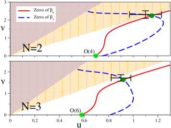
Figure 5: Some results for the RG flow of 3D O(2)$\otimes$O($N$) models obtained by the analysis of the five-loop $\overline{\rm MS}$ series [47]. The left figure shows the zeroes of the $\overline{\rm MS}$ $\beta$ functions. The right figure shows RG trajectories in the $u,v$ plane from the unstable Gaussian and O($2N$) FPs to the stable chiral FP for various values of the ratio $s\equiv v_{0}/u_{0}$ of the bare quartic parameters.

The RG flow of the O($M$)$\otimes$O($N$) $\Phi^{4}$ theory can be also studied analytically in the large-$N$ limit keeping fixed $M$, for any $2<d<4$. In the large-$N$ limit one finds four FPs as shown in Fig. 3, the stable FP is the chiral one denoted by the letter $C$. The values of the critical exponent $\eta$ at the FPs provide a further confirm of the $\eta$ conjecture [44], indeed setting $\eta={\eta_{1}e_{d}/N}+O(1/N^{2})$ where $e_{d}$ is a constant depending on $d$, one finds [51] $\eta_{1}=0$, $\eta_{1}=1/M$, $\eta_{1}=(M+1)/2$, and $\eta_{1}=(M-1)(M+2)/(2M)$ respectively for the Gaussian, O($M\times N$), chiral ad antichiral FPs. All numerical results at fixed $M,N$ satisfy the $\eta$ conjecture.

6 Ferromagnetic transitions in disordered spin systems

The FT approach allows us to also successfully describe ferromagnetic transitions in disordered spin systems, which are of considerable theoretical and experimental interest. Such transitions are observed in spin systems with impurities, such as mixing of antiferromagnetic materials with non magnetic ones, for example Fe_uZn_1-uF₂, Mn_uZn_1-uF₂ (uniaxial), Fe_xEr_z, Fe_xMn_yZr_z (isotropic), and also ⁴He in porous materials. See e.g. Refs. [54, 1, 55, 56] for experimental and theoretical reviews. These systems can be modeled by the lattice Hamiltonian

$$H_{\rho}=-J\,\sum_{\langle xy\rangle}\rho_{x}\,\rho_{y}\;\vec{s}_{x}\cdot\vec{s}_{y}$$ (21)

where the sum is over nearest-neighbor sites, $\vec{s}_{x}$ are $M$-component spin variables, and $\rho_{x}=1,0$ with probability $p$ and $1-p$, respectively. The disorder is quenched: it mimicks the physical situation in which the relaxation time of the diffusion of impurities is much larger than other typical scales. This implies that the free energy $F(\rho)\propto{\rm ln}Z(\rho)$ must be averaged over the disorder. Accordingly, the expectation value of an observable must be computed by

$$\langle{\cal O}\rangle(\beta,\{\rho\})={\sum_{\{s\}}{\cal O}e^{-\beta{\cal H}(s;\rho)}\over\sum_{\{s\}}e^{-\beta{\cal H}(s;\rho)}},\qquad\overline{\langle{\cal O}\rangle}=\int[d\rho]P(\rho)\langle{\cal O}\rangle(\beta,\{\rho\})$$

In the FT approach randomly-dilute spin models can be described by a $\Phi^{4}$ field theory for an $M$-component field $\Phi_{i}$ with and external random field $\psi(x)$ coupled to the energy-density operator:

$${\cal L}_{\psi}={1\over 2}\sum_{i}(\partial_{\mu}\Phi_{i}(x))^{2}+{1\over 2}(r+\psi(x))\sum_{i}\Phi_{i}(x)^{2}+{1\over 4!}g_{0}(\sum_{i}\Phi_{i}(x)^{2})^{2}$$ (22)

where $\psi(x)$ is a spatially uncorrelated random field, with probability $P(\psi)\sim{\rm exp}(-\psi^{2}/4w)$. Then, using the replica trick, ${\rm ln}Z={\rm lim}_{n\rightarrow 0}(Z^{n}-1)/n$, one can formally integrate over the disorder variables, arriving at a translation invariant $\Phi^{4}$ theory, which is the $MN$ model (15) with $u_{0}=-6w<0$. The critical behavior of the original system is determined by the RG flow of the $MN$ model in the nonunitary limit $N\rightarrow 0$. Therefore, it can be determined by analyzing the high-order MZM and $\overline{\rm MS}$ series for $N=0$, which have been computed respectively to six loops [26, 35, 34] and to five loops [33, 40].

An interesting physical issue is whether the presence of impurities, and in general of quenched disorder coupled to the energy density, can change the critical behavior. General RG arguments [52, 23] show that the asymptotic critical behavior remains unchanged if the specific-heat exponent $\alpha$ of the pure spin system is negative, which is the case of multicomponent O($M$)-symmetric spin systems, i.e. $M>1$. On the other hand, a different critical behavior is expected in the case of Ising-like systems ($M=1$), due to fact that $\alpha_{\rm Ising}=0.1096(5)$. This is confirmed by the results of the analyses of the high-order FT perturbative series, which show that the RG flow of the $MN$ model in the limit $N\rightarrow 0$ has a stable FP in the region $u<0$ when $M=1$, see Fig. 6, implying the existence of a 3D randomly-dilute Ising (RDIs) universality class.

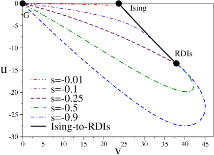
Figure 6: The RG flow of the $MN$ model for $M=1$ and $N\rightarrow 0$ in the quartic-coupling plane. It shows the trajectories from the unstable Gaussian and Ising FPs to the stable RDIs FP for various values of the ratio $s=u_{0}/v_{0}$ of the bare quartic parameters. Results obtained by the analysis of the six-loop MZM series [53].

Experiments, see, e.g., Refs. [54, 1] and references therein, confirm this scenario. The asymptotic critical behavior remains unchanged for multicomponent systems. Table 3 reports results for Ising-like systems: from experiments [54], the analysis of the six-loop FT expansion in the MZM scheme [35], and recent Monte Carlo simulations [57]. The global agreement is very good.

RDIs exponents	$\nu$	$\beta$
EXPT [54]	0.69(1)	0.359(9)
PFT 6-$l$ MZM [35]	0.678(10)	0.349(5)
MC [57]	0.683(2)	0.354(1)

Table 3: Results for the critical exponents of the 3D RDIs universality class.

It is worth mentioning that the RDIs universality class also describes ferromagnetic transitions in the presence of frustration, when frustration is not too large. This is for exmaple found in the 3D $\pm J$ Ising model [58], defined on a simple cubic lattice by the Hamiltonian

$$H_{\pm J}=-\sum_{\langle xy\rangle}J_{xy}\sigma_{x}\sigma_{y},\quad\sigma_{x}=\pm 1,$$ (23)

where $J_{xy}=\pm J$ with probability $P(J_{xy})=p\delta(J_{xy}-J)+(1-p)\delta(J_{xy}+J)$. This is a simplified model [59] for disordered and frustrated spin systems showing glass behavior in some region of their phase diagram. Unlike model (21), the $\pm J$ Ising model is frustrated for any $p$. Neverthless, the paramagnetic-ferromagnetic transition line extending for $1>p>p_{N}=0.76820(4)$ belongs to the RDIs universality class, i.e., frustration turns out to be irrelevant at this transition [58]. For $p<p_{N}$ the low-temperature phase is glassy with vanishing magnetization, thus the critical behavior at the transition belongs to a different Ising-glass universality class.

7 The finite-temperature transition in hadronic matter

The thermodynamics of Quantum Chromodynamics (QCD) is characterized by a transition at $T\simeq 200$ Mev from a low-$T$ hadronic phase, in which chiral symmetry is broken, to a high-$T$ phase with deconfined quarks and gluons (quark-gluon plasma), in which chiral symmetry is restored [60]. Our understanding of the finite-$T$ phase transition is essentially based on the relevant symmetry and symmetry-breaking pattern. In the presence of $N_{f}$ light quarks the relevant symmetry is the chiral symmetry ${\rm SU}(N_{f})_{L}\otimes{\rm SU}(N_{f})_{R}$. At $T=0$ this symmetry is spontaneously broken to SU($N_{f}$)_V with a nonzero quark condensate $\langle{\bar{\psi}}\psi\rangle$. The finite-$T$ transition is related to the restoring of the chiral symmetry. It is therefore characterized by the simmetry breaking

$${\rm SU}(N_{f})_{L}\otimes{\rm SU}(N_{f})_{R}\rightarrow{\rm SU}(N_{f})_{V}.$$ (24)

If the axial U(1)_A symmetry is effectively restored at $T_{c}$, the expected symmetry breaking becomes

$${\rm U}(N_{f})_{L}\otimes{\rm U}(N_{f})_{R}\rightarrow{\rm U}(N_{f})_{V}.$$ (25)

A suppression of the anomaly effects at $T_{c}$ is however unlikely in QCD. Semiclassical calculations in the high-temperature phase [61] show that instantons are exponentially suppressed for $T\gg T_{c}$, implying a suppression of the anomaly effects in the high-temperature limit. Some lattice studies [62] suggest a significant reduction of the effective U(1)_A symmetry breaking around $T_{c}$, but not a complete suppression. Since the anomaly, $\partial_{\mu}J_{5}^{\mu}\propto{1\over N_{c}}Q$, gets suppressed in the large-$N_{c}$ limit, the symmetry-breaking pattern (25) may be relevant in the large-$N_{c}$ limit.

Other interesting QCD-like theories are ${\rm SU}(N_{c})$ gauge theories with $N_{f}$ Dirac fermions in the adjoint representation (aQCD). They are asymptotically free only for $N_{f}<11/4$, thus only the cases $N_{f}=1,2$ are interesting. Unlike QCD, aQCD is also invariant under global ${\mathbb{Z}}_{N_{c}}$ transformations related to the center of the gauge group SU($N_{c}$), as in pure ${\rm SU}(N_{c})$ gauge theories. There are two well-defined order parameters in the light-quark regime, related to the confining and chiral modes, i.e. the Polyakov loop and the quark condensate. Therefore, one generally expects two transitions: a deconfinement transition at $T_{d}$ associated with the breaking of the ${\mathbb{Z}}_{N_{c}}$ symmetry, and a chiral transition at $T_{c}$ in which chiral symmetry is restored. In aQCD with $N_{f}$ massless flavors the chiral-symmetry group extends to  [63] ${\rm SU}(2N_{f})$. At $T=0$ this symmetry is expected to spontaneously break to ${\rm SO}(2N_{f})$, due to quark condensation. Therefore the symmetry breaking at the finite-$T$ chiral transition is

$${\rm SU}(2N_{f})\rightarrow{\rm SO}(2N_{f})$$ (26)

with a symmetric $2N_{f}\times 2N_{f}$ complex matrix as order parameter related to the bilinear quark condensate. If the axial U(1)_A symmetry is restored at $T_{c}$, the symmetry-breaking pattern is ${\rm U}(2N_{f})\rightarrow{\rm O}(2N_{f})$. MC simulations for $N_{c}=3$ and $N_{f}=2$ [64, 65] show that the deconfinement transition at $T_{d}$ is first order, while the chiral transition appears continuous. The ratio between the two critical temperatures turns out to be quite large: $T_{c}/T_{d}\approx 8$.

	U(1)A anomaly	suppressed anomaly at $T_{c}$
QCD	${\rm SU}(N_{f})_{L}\otimes{\rm SU}(N_{f})_{R}\rightarrow{\rm SU}(N_{f})_{V}$	${\rm U}(N_{f})_{L}\otimes{\rm U}(N_{f})_{R}\rightarrow{\rm U}(N_{f})_{V}$
$N_{f}=1$	crossover or first order	O(2) or first order
$N_{f}=2$	O(4) or first order	U(2)${}_{L}\otimes$U(2)R/U(2)V or first order
$N_{f}\geq 3$	first order	first order
aQCD	${\rm SU}(2N_{f})\rightarrow{\rm SO}(2N_{f})$	${\rm U}(2N_{f})\rightarrow{\rm O}(2N_{f})$
$N_{f}=1$	O(3) or first order	U(2)/O(2) or first order
$N_{f}=2$	SU(4)/SO(4) or first order	first order

Table 4: Summary of the RG predictions. We report the possible types of transition for each case, indicating the universality class when the transition can also be continuous.

In order to study the nature of the finite-$T$ chiral transition in QCD and aQCD, one can exploit universality and renormalization-group (RG) arguments. [66, 37, 41, 67]

• Let us first assume that the phase transition at $T_{c}$ is continuous for vanishing quark masses. In this case the length scale of the critical modes diverges approaching $T_{c}$, becoming eventually much larger than $1/T_{c}$, which is the size of the euclidean “temporal” dimension at $T_{c}$. Therefore, the asymptotic critical behavior must be associated with a 3D universality class with the same symmetry breaking. The order parameter must be an $N_{f}\times N_{f}$ complex-matrix field $\Phi_{ij}$, related to the bilinear quark operators $\bar{\psi}_{Li}\psi_{Rj}$.

• The existence of such a 3D universality class can be investigated by considering the most general LGW $\Phi^{4}$ theory compatible with the given symmetry breaking, which describes the critical modes at $T_{c}$. Neglecting the U(1)_A anomaly, it is given by

  $${\cal L}_{{\rm U}(N)}={\rm Tr}(\partial_{\mu}\Phi^{\dagger})(\partial_{\mu}\Phi)+r{\rm Tr}\Phi^{\dagger}\Phi+{u_{0}\over 4}\left({\rm Tr}\Phi^{\dagger}\Phi\right)^{2}+{v_{0}\over 4}{\rm Tr}\left(\Phi^{\dagger}\Phi\right)^{2}.$$ (27)

  If $\Phi_{ij}$ is a generic $N\times N$ complex matrix, the symmetry is U$(N)_{L}\otimes$U$(N)_{R}$, which breaks to U$(N)_{V}$ if $v_{0}>0$, thus providing the LGW theory relevant for QCD with $N_{f}=N$. If $\Phi_{ij}$ is also symmetric, the global symmetry is U$(N)$, which breaks to O($N$) if $v_{0}>0$, which is the case relevant for aQCD with $N_{f}=N/2$. The reduction of the symmetry to SU$(N_{f})_{L}\otimes$SU$(N_{f})_{R}$ for QCD [SU$(2N_{f})$ for aQCD], due to the axial anomaly, is achieved by adding determinant terms, such as

  $${\cal L}_{{\rm SU}(N)}={\cal L}_{{\rm U}(N)}+w_{0}\left({\rm det}\Phi^{\dagger}+{\rm det}\Phi\right).$$ (28)

  Nonvanishing quark masses can be accounted for by adding an external-field term ${\rm Tr}\left(H\Phi+{\rm h.c.}\right)$.

• The critical behavior at a continuous transition is determined by the FPs of the RG flow: the absence of a stable FP generally implies first-order transitions. Therefore, a necessary condition of consistency with the initial hypothesis (i) of a continuous transition is the existence of stable FP in the corresponding LGW $\Phi^{4}$ theory. If no stable FP exists, the finite-$T$ chiral transition of QCD (aQCD) is predicted to be first order. If a stable FP exists, the transition can be continuous, and its critical behavior is determined by the FP; but this does not exclude a first-order transition if the system is outside the attraction domain of the stable FP.

Figure 7: Zeroes of the $\beta$-functions associated with the quartic couplings of the Lagrangian (27) for $N=2$ (from Ref. [67]).

The above RG arguments show that the nature of the finite-$T$ transition in QCD and aQCD can be investigated by studying the RG flow of the corresponding 3D LGW $\Phi^{4}$ field theories. RG studies based on high-order perturbative calculations in the MZM and $\overline{\rm MS}$ are reported in Refs. [37, 41, 67]. Table 4 presents a summary of the predictions obtained by these RG analyses for the finite-$T$ chiral transitions in QCD and aQCD with $N_{f}$ massless quarks.

The case relevant to $N_{f}=1$ QCD, i.e. the Lagrangian (27) with $N=1$, reduces to the O(2) symmetric $\Phi^{4}$ theory, corresponding to the 3D $XY$ universality class. The determinant term related to the axial anomaly, cf. Eq. (28), plays the role of an external field, thus no continuous transition is expected, but a crossover.

In the case relevant for $N_{f}=2$ QCD with suppressed U(1)_A anomaly, i.e. the $\Phi^{4}$ theory (27) with $N=2$, the analyses of both MZM and 3D $\overline{\rm MS}$ schemes provide a robust evidence of a stable FP, see Fig. 7. A corresponding 3-D U(2)$\otimes$U(2)/U(2) universality class exists, with critical exponents $\nu\approx 0.7$ and $\eta\approx 0.1$. No stable FP is found close to $d=4$ by one-loop $\epsilon$-expansion calculations [66], but, as already remarked in Sec. 5, the extension to $d=3$ of $\epsilon$-expansion results may fail. A stable FP is also found when the field $\Phi$ is symmetric, which is relevant for aQCD with one flavor, thus showing the existence of a universality class characterized by the simmetry breaking U(2)$\rightarrow$O(2).

In two-flavor QCD, taking into account the U(1)_A anomaly, the symmetry breaking (24) becomes equivalent to the one of the O(4) vector universality class, i.e. O(4)$\rightarrow$O(3). The symmetry breaking (26) of $N_{f}=1$ aQCD is instead equivalent to the one of the O(3) vector universality class. This already suggests that, if the transition in the chiral limit of $N_{f}=2$ QCD is continuous, it must show the same asymptotic behavior of the 3D O(4) universality class (O(3) in the case of $N_{f}=1$ aQCD). This implies that the critical equation of state of the 3D O(4) universality class,

$$\vec{M}\propto\vec{H}|H|^{(1-\delta)/\delta}E(y),\qquad y\propto t|H|^{-1/(\beta+\delta)},$$ (29)

provides a scaling relation between the quark condensate $\langle\bar{\psi}\psi\rangle$, and the quark mass $m_{f}$, which correspond respectively to the magnetization $M$ and the external field $H$. The critical equation of state of the 3D O(4) universality class has been accurately determined in the 3D O(4) vector model: the critical exponents are [68] $\delta=4.789(6)$, $\beta=0.3882(10)$, and the universal scaling function $E(y)$ is shown in Fig. 8.

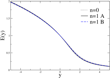
Figure 8: The scaling function $E(y)$ for the O(4) universality class, from Ref. [69]. The different lines represent different approximations.

Actually, the LGW $\Phi^{4}$ theory corresponding to $N_{f}=2$ QCD is quite complicated [37, 67]:

$${\cal L}_{{\rm SU}(2)}={\rm Tr}(\partial_{\mu}\Phi^{\dagger})(\partial_{\mu}\Phi)+r{\rm Tr}\Phi^{\dagger}\Phi+{u_{0}\over 4}\left({\rm Tr}\Phi^{\dagger}\Phi\right)^{2}+{v_{0}\over 4}{\rm Tr}\left(\Phi^{\dagger}\Phi\right)^{2}+$$ (30)

$$+w_{0}\left({\rm det}\Phi^{\dagger}+{\rm det}\Phi\right)+{x_{0}\over 4}\left({\rm Tr}\Phi^{\dagger}\Phi\right)\left({\rm det}\Phi^{\dagger}+{\rm det}\Phi\right)+{y_{0}\over 4}\left[({\rm det}\Phi^{\dagger})^{2}+({\rm det}\Phi)^{2}\right],$$

where $w_{0},x_{0},y_{0}\sim g$ and $g$ parametrizes the effective breaking of the U(1)_A symmetry. If the anomaly is suppressed ($g=0$), then $w_{0}=x_{0}=y_{0}=0$. ${\cal L}_{{\rm SU}(2)}$ contains two quadratic (mass) terms, therefore it describes several transition lines in the $T$-$g$ plane, which meet at a multicritical point for $g=0$. In the case of QCD the multicritical behavior is controlled by the U(2)_L$\otimes$U(2)_R symmetric theory. Possible phase diagrams in the $T$-$g$ plane are shown in Fig. 9. When $g\neq 0$ the transition may be first order or continuous in the O(4) universality class. Actually, we may also have a mean-field behavior (apart from logarithms) for particular values of $g$, see Fig. 9. If $|g|$ is small (a partial suppression of anomaly effects around $T_{c}$ is suggested by MC simulations [62]) we may observe crossover effects controlled by the U(2)$\otimes$U(2) multicritical point at $g=0$: if the transition is continuous at $g=0$ then the free-energy should behave as ${\cal F}_{\rm sing}\approx t^{3\nu}f(gt^{-\phi})$, where $t\propto T-T_{c}(g=0)$, $\nu\approx 0.7$, $\phi\approx 1.5$. If the transition is first order at $g=0$, then it is expected to remain first order for small $g$. A similar scenario applies also to $N_{f}=1$ aQCD.

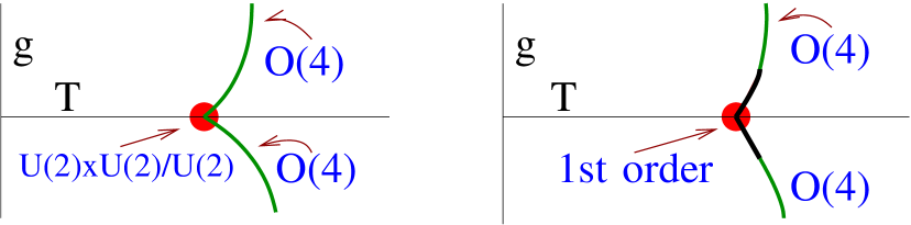
Figure 9: Possible phase diagrams in the $T$-$g$ plane for the LGW theory (30) describing the transition of $N_{f}=2$ QCD, in the case the transition at the multicritical point, i.e. for $g=0$, is continuous (left) or first order (right). Thick black lines indicate first-order transitions. At their end points, thus for particular values of $g$, the transition should be of mean-field type (apart from logarithms).

No stable FPs are found for $N>2$ in the LGW theory (27). Thus, neglecting the anomaly, transitions are always first order when $N_{f}>2$ for QCD and $N_{f}>1$ for aQCD. In most cases this result does not change if we take into account the axial anomaly, cf. Eq. (28). The only exception is the case related to $N_{f}=2$ aQCD, where a stable FP is found [41], corresponding to a 3D SU(4)/SO(4) universality class, with critical exponents $\nu\approx 1.1$ and $\eta\approx 0.2$.

In nature quarks are not massless, although some of them, the quarks $u$ and $d$, are light. The physically interesting case is QCD with $N_{f}=2$ light quarks and four heavier quarks (in particular the quark $s$ with $m_{s}\approx 100$ Mev). Therefore, it is important to consider the effects of the quark masses in the above transition scenarios. According to the above RG arguments, if the transition is continuous in the chiral limit then an analytic crossover is expected for nonzero values of the quark masses $m_{f}$, because the quark masses act as external fields in the corresponding LGW $\Phi^{4}$ theories. On the other hand, a first-order transition is generally robust against perturbations, and therefore it is expected to persist for $m_{f}>0$, up to an Ising end point. Actually, the presence of the massive quark $s$ makes the above scenario more complicated, because the nature of the transition may be sensitive to its mass $m_{s}$. Since the transition is expected to be first order in the chiral limit of $N_{f}=3$ degenerate quarks, we also expect that the first-order transition persists for sufficiently small value of $m_{s}$. On the other hand, if the transition is continuous in the limit $m_{s}\rightarrow\infty$ corresponding to $N_{f}=2$ degenerate quarks, then there must be a tricritical point at $m_{s}=m_{s}^{*}$ (where the critical behavior is mean field apart logarithms) separating the first-transition line from the O(4) critical line.

The nature of the transition in QCD can be investigated by lattice MC simulations. For $m_{f}>0$ around their physical values, MC simulations show that the low-$T$ hadronic and high-$T$ quark-gluon plasma regimes are not separated by a phase transition, but by an analytic crossover where the thermodynamic quantities change rapidly in a relatively narrow temperature interval, see, e.g., Refs. [70, 71, 72, 73, 74]. Neverthless, the nature of the transition in the chiral limit is still of interest. Since the physical masses of the lightest quarks $u$ and $d$ are very small, some scaling relations may still be valid at the physical values of the quark masses, such as, for example, the O(4) relation (29) between the quark condensate and masses in the case the phase transition in the chiral limit is continuous and belongs to the O(4) universality class.

The numerical investigation of the transition in the chiral limit is a hard task because it must be studied in the infinite-volume limit ($V\rightarrow\infty$), in the continuum limit ($N_{t}\rightarrow\infty$ where $N_{t}$ is the number of lattice spacings along the Euclidean time direction), and massless limit ($m_{f}\rightarrow 0$). A robust control of the scaling corrections related to the continuum limit is essential. One cannot even exclude that in some lattice formulations the nature of the transition changes when approaching the continuum limit. Moreover, in the case of a continuous transition, the scaling corrections in the r.h.s. of Eq. (5) may hide the universal asymptotic behavior if MC simulations are not done sufficiently close to the critical point (for example, in the case of the O(4) universality class, the leading scaling-correction exponent is not large, i.e. $\Delta\simeq 0.5$).

In the case of $N_{f}=2$ light quarks, the RG prediction for the chiral transition is that it is first order or a continuous transition in the 3D O(4) universality class. Many studies based on MC simulations of different lattice formulations of QCD have been performed, see e.g. Refs. [75, 76, 77, 78, 79, 80, 81], but this issue is still controversial. Some MC results favor a continuous transition. However, the results have not been sufficient to settle its O(4) nature yet. There are also results indicating a first-order transition. Unlike $N_{f}=2$ QCD, the transition scenario appears settled for $N_{f}\geq 3$: MC simulations [77, 82, 83, 84, 73] show first-order transitions, in agreement with the RG predictions. Finally, in the case of $N_{f}=2$ aQCD the available MC results [64, 65] favor a continuous transitions. But they are not yet sufficiently precise to check the critical behavior of the 3D SU(4)/SO(4) universality class.

References

- [1] A. Pelissetto, E. Vicari, Phys. Rep. 368 (2002) 549 [arXiv:cond-mat/0012164].
- [2] J. Zinn-Justin, Quantum Field Theory and Critical Phenomena, (Clarendon Press, Oxford, 1989), fourth edition Oxford 2002.
- [3] L.D. Landau, Phys. Z. Sowjetunion 11 (1937) 26; 11 (1937) 545.
- [4] K.G. Wilson, Phys. Rev. B 4 (1971) 3174; Phys. Rev. B 4 (1971) 3184.
- [5] K.G. Wilson, J. Kogut, Phys. Rep. 12 (1974) 77.
- [6] M.E. Fisher, Rev. Mod. Phys. 46 (1974) 597.
- [7] K. G. Wilson, Phys. Rev. D 10 (1974) 2445; Quarks and Strings on a Lattice, in New Phenomena in Subnuclear Physics, edited by A. Zichichi (Plenum Press, New York, 1975).
- [8] C. Bagnuls, C. Bervillier, Phys. Rev. B 32 (1985) 7209.
- [9] G. Parisi, Cargèse Lectures (1973), J. Stat. Phys. 23 (1980) 49.
- [10] G. A. Baker, Jr., B. G. Nickel, M. S. Green, D. I. Meiron, Phys. Rev. Lett. 36 (1977) 1351; D. B. Murray, B. G. Nickel, Revised estimates for critical exponents for the continuum -vector model in 3 dimensions, unpublished Guelph University report (1991).
- [11] A. Pelissetto, E. Vicari, Nucl. Phys. B 519 (1998) 626 [arXiv:cond-mat/9801098].
- [12] J.C. Le Guillou, J. Zinn-Justin, Phys. Rev. Lett. 39 (1977) 95; Phys. Rev. B 21 (1980) 3976.
- [13] G. ’t Hooft, M.J.G. Veltman, Nucl. Phys. B 44 (1972) 189.
- [14] K. G. Wilson, M. E. Fisher, Phys. Rev. Lett. 28 (1972) 240.
- [15] V. Dohm, Z. Phys. B 60 (1985) 61; B 61 (1985) 193; R. Schloms, V. Dohm, Nucl. Phys. B 328 (1989) 639.
- [16] R. Guida, J. Zinn-Justin, J. Phys A 31 (1998) 8103 [arXiv:cond-mat/9803240].
- [17] M. Campostrini, A. Pelissetto, P. Rossi, E. Vicari, Phys. Rev. E 65 (2002) 066127 [arXiv:cond-mat/0201180].
- [18] Y. Deng, H.W.J. Blöte, Phys. Rev. E 68 (2003) 036125.
- [19] J.A. Lipa, D.R. Swanson, J.A. Nissen, T.C.P. Chui, and U.E. Israelsson, Phys. Rev. Lett. 76 (1996) 944; J.A. Lipa, D.R. Swanson, J.A. Nissen, Z.K. Geng, P.R. Williamson, D.A. Stricker, T.C.P. Chui, U.E. Israelsson, and M. Larson, Phys. Rev. Lett. 84 (2000) 4894; J.A. Lipa, J.A. Nissen, D.A. Stricker, D.R. Swanson, T.C.P. Chui, Phys. Rev. B B 68 (2003) 174518.
- [20] M. Campostrini, M. Hasenbusch, A. Pelissetto, E. Vicari, Phys. Rev. B 74 (2006) 144506 [arXiv:cond-mat/0605083].
- [21] E. Burovski, J. Machta, N. Prokof’ev, B. Svistunov, Phys. Rev. B 74 (2006) 132502 [arXiv:cond-mat/0507352].
- [22] J.A. Lipa, S Wang, J.A. Nissen, D. Avaloff, Advances in Space Research 36 (2005) 119.
- [23] A. Aharony, in Phase Transitions and Critical Phenomena, C. Domb and M.S. Green eds. (Academic Press, New York, 1976), Vol. 6, p. 357.
- [24] E. Brézin, J.C. Le Guillou, J. Zinn-Justin, in Phase Transitions and Critical Phenomena, C. Domb and M.S. Green eds. (Academic Press, New York, 1976), Vol. 6, p. 125.
- [25] E. Brézin, J.C. Le Guillou, J. Zinn-Justin, Phys. Rev. B 10 (1974) 893.
- [26] J. Carmona, A. Pelissetto, E. Vicari, Phys. Rev. B 61 (2000) 15136 [arXiv:cond-mat/9912115].
- [27] Y. Zhang, E. Demler, S. Sachdev, Phys. Rev. B 66 (2002) 094501 [arXiv:cond-mat/0112343].
- [28] M. De Prato, A. Pelissetto, E. Vicari, Phys. Rev. B 74 (2006) 144507 [arXiv:cond-mat/0601404].
- [29] D.R. Nelson, J.M. Kosterlitz, M.E. Fisher, Phys. Rev. Lett. 33 (1974) 813; J.M. Kosterlitz, D.R. Nelson, M.E. Fisher, Phys. Rev. B 13 (1976) 412.
- [30] P. Calabrese, A. Pelissetto, E. Vicari, Phys. Rev. B 67 (2003) 054505 [arXiv:cond-mat/0209580].
- [31] M. Hasenbusch, A. Pelissetto, E. Vicari, Phys. Rev. B 72 (2005) 014532 [arXiv:cond-mat/0502327].
- [32] A. Pelissetto, E. Vicari, Phys. Rev. B 76 (2007) 024436 [arXiv:cond-mat/0702273].
- [33] H. Kleinert, V. Schulte-Frohlinde, Phys. Lett. B 342 (1995) 284.
- [34] D.V. Pakhnin, A.I. Sokolov, Phys. Rev. B 61 (2000) 15130 [arXiv:cond-mat/9912071].
- [35] A. Pelissetto, E. Vicari, Phys Rev. B 62 (2000) 6393 [arXiv:cond-mat/0002402].
- [36] A. Pelissetto, P. Rossi, E. Vicari, Phys. Rev. B 63 (2001) 140414(R) [arXiv:cond-mat/0007389].
- [37] A. Butti, A. Pelissetto, E. Vicari, JHEP 08 (2003) 029 [arXiv:hep-ph/0307036].
- [38] P. Calabrese, P. Parruccini, Nucl. Phys. B 679 (2004) 568 [arXiv:cond-mat/0308037].
- [39] P. Calabrese, P. Parruccini, JHEP 05 (2004) 018 [arXiv:hep-ph/0403140].
- [40] A. Pelissetto, E. Vicari, Condensed Matter Physics (Ukraine) 8 (2005) 87 [arXiv:hep-th/0409214].
- [41] F. Basile, A. Pelissetto, E. Vicari, JHEP 02 (2005) 044 [arXiv:hep-th/041202].
- [42] A.B. Zamolodchikov, Pis’ma Zh. Eksp. Teor. Fiz. 43 (1986) 565; JETP Lett. 43 (1986) 730.
- [43] J. Cardy. Phys. Lett. B 215 (1989) 749; S. Forte, J.I. Latorre, Nucl. Phys. B 535 (1998) 709 [arXiv:hep-th/9805015]; D. Anselmi, Annals Phys. 276 (1999) 361 [arXiv:hep-th/9903059]; A. Cappelli, G. D’Appollonio, Phys. Lett. B 487 (2000) 87 [arXiv:hep-th/0005115]; A. Cappelli, R. Guida, N. Magnoli Nucl. Phys. B 618 (2001) 371 [arXiv:hep-th/0103237].
- [44] E. Vicari, J. Zinn-Justin, New Journal of Physics 8 (2006) 321 [arXiv:cond-mat/0611353].
- [45] H. Kawamura, J. Phys.: Condens. Matter 10 (1998) 4707 [arXiv:cond-mat/9805134].
- [46] B. Delamotte, D. Mouhanna, M. Tissier, Phys. Rev. B 69 (2004) 134413 [arXiv:cond-mat/0309101].
- [47] P. Calabrese, P. Parruccini, A. Pelissetto, E. Vicari, Phys. Rev. B 70 (2004) 174439 [arXiv:cond-mat/0405667].
- [48] M. De Prato, A. Pelissetto, E. Vicari, Phys. Rev. B 70 (2004) 214519 [arXiv:cond-mat/0312362].
- [49] P. Calabrese, P. Parruccini, A.I. Sokolov, Phys. Rev. B 66 (2002) 180403 [arXiv:cond-mat/0205046].
- [50] A. Peles, B.W. Southern, Phys. Rev. B 67 (2003) 184407 [arXiv:cond-mat/0209056].
- [51] A. Pelissetto, P. Rossi, E. Vicari, Nucl. Phys. B 607 (2001) 605 [arXiv:hep-th/0104024].
- [52] A.B. Harris, J. Phys. C 7 (1974) 1671.
- [53] P. Calabrese, P. Parruccini, A. Pelissetto, E. Vicari, Phys. Rev. E 69 (2004) 036120 [arXiv:cond-mat/0307699].
- [54] D.P. Belanger, Braz. J. Phys. 30 (2000) 682 [arXiv:cond-mat/0009029].
- [55] R. Folk, Yu. Holovatch, T. Yavors’kii, Uspekhi Fiz. Nauk 173 (2003) 175 [Phys. Usp. 46 (2003) 175] [arXiv:cond-mat/0106468].
- [56] W. Janke, B. Berche, C. Chatelain, P.E. Berche, M. Hellmund, PoS (LAT2005) 018.
- [57] M. Hasenbusch, F. Parisen Toldin, A. Pelissetto, E. Vicari, J. Stat. Mech.: Theory Exp. (2007) P02016 [arXiv:cond-mat/0611707].
- [58] M. Hasenbusch, F. Parisen Toldin, A. Pelissetto, E. Vicari, Phys. Rev. B 76 (2007) 094402 [arXiv:0704.0427]; Phys. Rev. B in press [arXiv:0707.2866].
- [59] S.F. Edwards, P.W. Anderson, J. Phys. F 5 (1975) 965.
- [60] See, e.g., F. Wilczek, QCD in extreme conditions, arXiv:hep-ph/0003183; F. Karsch, Lect. Notes Phys. 583 (2002) 209 [arXiv:hep-lat/0106019].
- [61] D.J. Gross, R.D. Pisarski, L.G. Yaffe, Rev. Mod. Phys. 53 (1981) 43.
- [62] C. Bernard, T. Blum, C. DeTar, S. Gottlieb, U.M. Heller, J.E. Hetrick, K. Rummukainen, R. Sugar, D. Toussaint, M. Wingate, Phys. Rev. Lett. 78 (1997) 598 [arXiv:hep-lat/9611031]; J. B. Kogut, J.-F. Lagaë, D. K. Sinclair, Phys. Rev. D 58 (1998) 054504 [arXiv:hep-lat/9801020]; P. M. Vranas, Nucl. Phys. (Proc. Suppl.) 83 (2000) 414 [arXiv:hep-lat/9911002].
- [63] A. Smilga, J.J.M. Verbaarschot, Phys. Rev. D 51 (1995) 829.
- [64] F. Karsch, M. Lütgemeier, Nucl. Phys. B 550 (1999) 449 [arXiv:hep-lat/9812023].
- [65] J. Engels, S. Holtmann, T. Schulze, Nucl. Phys. B 724 (2005) 357 [arXiv:hep-lat/0505008]; PoS (LAT2005) 148 [arXiv:hep-lat/0509010].
- [66] R.D. Pisarski, F. Wilczek, Phys. Rev. D 29 (1984) 338.
- [67] F. Basile, A. Pelissetto, E. Vicari, PoS (LAT2005) 199 [arXiv:hep-lat/0509018].
- [68] M. Hasenbusch, J. Phys. A 34 (2001) 8221 [arXiv:cond-mat/0010463].
- [69] F. Parisen Toldin, A. Pelissetto, E. Vicari, JHEP 07 (2003) 029 [arXiv:hep-ph/0305264].
- [70] C. Bernard et al [MILC collaboration], Phys. Rev. D 71 (2005) 034504 [arXiv:hep-lat/0405029].
- [71] M. Cheng, N. H. Christ, S. Datta, J. van der Heide, C. Jung, F. Karsch, O. Kaczmarek, E. Laermann, R. D. Mawhinney, C. Miao, P. Petreczky, K. Petrov, C. Schmidt, T. Umeda, Phys. Rev. D 74 (2006) 054507 [arXiv:hep-lat/0608013].
- [72] Y. Aoki, Z. Fodor, S.D. Katz, K.K. Szabo, Phys. Lett. B 643 (2006) 46 [arXiv:hep-lat/0609068]; Y. Aoki, G. Endrodi, Z. Fodor, S.D. Katz, K.K. Szabo, Nature 443 (2006) 675 [arXiv:hep-lat/0611014].
- [73] P. de Forcrand, O. Philipsen, JHEP 01 (2007) 077 [arXiv:hep-lat/0607017].
- [74] F. Karsch, talk at this conference; Z. Fodor, talk at this conference.
- [75] A. Ali Khan et al. (CP-PACS Collaboration), Phys. Rev. D 63 (2001) 034502 [arXiv:hep-lat/0008011].
- [76] C.W. Bernard, et. al [MILC collaboration], Phys. Rev. D 61 (2000) 111502 [arXiv:hep-lat/9912018].
- [77] F. Karsch, E. Laermann, A. Peikert, Nucl. Phys. B 605 (2001) 579 [arXiv:hep-lat/0012023].
- [78] J. B. Kogut, D. K. Sinclair, Phys. Rev. D 64 (2001) 034508 [arXiv:hep-lat/0104011].
- [79] J. Engels, S. Holtmann, T. Mendes, T. Schulze, Phys. Lett. B 514 (2001) 299 [arXiv:hep-lat/0105028].
- [80] M. D’Elia, A. Di Giacomo, C. Pica, Phys. Rev. D 72 (2005) 114510 [arXiv:hep-lat/0503030]; G. Cossu, M. D’Elia, A. Di Giacomo, C. Pica, arXiv:0706.4470.
- [81] J.B. Kogut, D.K. Sinclair, Phys. Rev. D 73 (2006) 074512 [arXiv:hep-lat/0603021].
- [82] Y. Iwasaki, K. Kanaya, S. Sakai, T. Yoshié, Z. Physik C 71 (1996) 337 [arXiv:hep-lat/9504019].
- [83] P. de Forcrand, O. Philipsen, Nucl. Phys. B 673 (2003) 170 [arXiv:hep-lat/0307020].
- [84] M. Cheng, N. H. Christ, M.A. Clark, J. van der Heide, C. Jung, F. Karsch, O. Kaczmarek, E. Laermann, R. D. Mawhinney, C. Miao, P. Petreczky, K. Petrov, C. Schmidt, W. Soeldner, T. Umeda, Phys. Rev D 75 (2007) 034506 [arXiv:hep-lat/0612001].