Short-time critical dynamics of the three-dimensional systems with long-range correlated disorder

Abstract

Monte Carlo simulations of the short-time dynamic behavior are reported for three-dimensional Ising and XY models with long-range correlated disorder at criticality, in the case corresponding to linear defects. The static and dynamic critical exponents are determined for systems starting separately from ordered and disordered initial states. The obtained values of the exponents are in a good agreement with results of the field-theoretic description of the critical behavior of these models in the two-loop approximation and with our results of Monte Carlo simulations of three-dimensional Ising model in equilibrium state.

I Introduction

The investigation of critical behavior of disordered systems remains one of the main problems in condensed matter physics and excites a great interest, because all real solids contain structural defects. The structural disorder breaks the translational symmetry of the crystal and thus greatly complicates the theoretical description of the material. The influence of disorder is particularly important near critical point where behavior of a system is characterized by anomalous large response on any even weak perturbation. In most investigations consideration has been restricted to the case of point-like uncorrelated defects 1 . However, the non-idealities of structure cannot be modeled by simple uncorrelated defects only. Solids often contain defects of a more complex structure: linear dislocations, planar grain boundaries, clusters of point-like defects, and so on.

Different models of structural disorder have arisen as an attempt to describe such complicated defects. In this paper we concentrate on model of Weinrib and Halperin (WH) 2 with the so-called long-range correlated disorder when pair correlation function for point-like defects $g({\bf x}-{\bf y})$ falls off with distance as a power law $g({\bf x}-{\bf y})\sim|{\bf x-y}|^{-a}$. Weinrib and Halperin showed that for $a\geq d$ long-range correlations are irrelevant and the usual short-range Harris criterion 3 $2-d\nu_{0}=\alpha_{0}>0$ of the effect of point-like uncorrelated defects is realized, where $d$ is the spatial dimension, and $\nu_{0}$ and $\alpha_{0}$ are the correlation-length and the specific-heat exponents of the pure system. For $a<d$ the extended criterion $2-a\nu_{0}>0$ of the effect of disorder on the critical behavior was established. As a result, a wider class of disordered systems, not only the three-dimensional diluted Ising model with point-like uncorrelated defects, can be characterized by a new type of critical behavior. So, for $a<d$ a new long-range (LR) disorder stable fixed point (FP) of the renormalization group recursion relations for systems with a number of components of the order parameter $m\geq 2$ was discovered. The critical exponents were calculated in the one-loop approximation using a double expansion in $\varepsilon=4-d\ll 1$ and $\delta=4-a\ll 1$. The correlation-length exponent was evaluated in this linear approximation as $\nu=2/a$ and it was argued that this scaling relation is exact and also holds in higher order approximation. In the case $m=1$ the accidental degeneracy of the recursion relations in the one-loop approximation did not permit to find LR disorder stable FP. Korzhenevskii et al 4 proved the existence of the LR disorder stable FP for the one-component WH model and also found characteristics of this type of critical behavior.

Ballesteros and Parisi 5 have studied by Monte Carlo means the critical behavior in equilibrium of the 3D site-diluted Ising model with LR spatially correlated disorder, in the $a=2$ case corresponding to linear defects. They have computed the critical exponents of these systems with the use of the finite-size scaling techniques and found that a $\nu$ value is compatible with the analytical predictions $\nu=2/a$.

However, numerous investigations of pure and disordered systems performed with the use of the field-theoretic approach show that the predictions made in the one-loop approximation, especially based on the $\varepsilon$ - expansion, can differ strongly from the real critical behavior 6 ; 7 ; 8 ; 9 . Therefore, the results for WH model with LR correlated defects received based on the $\varepsilon,\delta$ - expansion 2 ; 4 ; 10 ; 11 ; 12 was questioned in our paper 13 , where a renormalization analysis of scaling functions was carried out directly for the 3D systems in the two-loop approximation with the values of $a$ in the range $2\leq a\leq 3$, and the FPs corresponding to stability of various types of critical behavior were identified. The static and dynamic critical exponents in the two-loop approximation were calculated with the use of the Pade-Borel summation technique. The results obtained in 13 essentially differ from the results evaluated by a double $\varepsilon,\delta$ - expansion. The comparison of calculated the exponent $\nu$ values and ratio $2/a$ showed the violation of the relation $\nu=2/a$, supposed in 2 as exact.

The models with LR-correlated quenched defects have both theoretical interest due to the possibility of predicting new types of critical behavior in disordered systems and experimental interest due to the possibility of realizing LR-correlated defects in the orientational glasses 14 , polymers 15 , and disordered solids containing fractal-like defects 4 or dislocations near the sample surface 16 .

To shed light on the reason of discrepancy between the results of Monte Carlo simulation of the 3D Ising model with LR-correlated disorder 5 , in the $a=2$ case, and the results of our renormalization group description of this model 13 , we have computed by the short-time dynamics method 17 ; 18 the static and dynamic critical exponents for site-diluted 3D Ising and XY models with the linear defects of random orientation in a sample.

In the following section, we introduce a site-diluted 3D Ising model with the linear defects and scaling relations for the short-time critical dynamics. In Section III, we give results of critical temperature determination for 3D Ising model with the linear defects for case with spin concentration $p=0.8$. We analyze the critical short-time dynamics in Ising systems starting separately from ordered and disordered initial states. Critical exponents obtained under these two conditions with the use of the corrections to scaling are compared. Also, in Section III the results of measurements of the critical characteristics for 3D Ising model in equilibrium state are presented in comparison with results of the short-time dynamics method. In Section IV the results of Monte Carlo studies of critical behavior of 3D XY-model with linear defects for the same spin concentration $p=0.8$ are considered. Our main conclusions are discussed in Section V.

II Model and Methods

We have considered the following Ising model Hamiltonian defined in a cubic lattice of linear size $L$ with periodic boundary conditions:

$$H=-J\sum_{\langle i,j\rangle}p_{i}p_{j}S_{i}S_{j},$$ (1)

where the sum is extended to the nearest neighbors, $S_{i}=\pm 1$ are the usual spin variables, and the $p_{i}$ are quenched random variables ($p_{i}=1$, when the site $i$ is occupied by spin, and $p_{i}=0$, when the site is empty), with LR spatial correlation. An actual $p_{i}$ set will be called a sample from now on. We have studied the next way to introduce the correlation between the $p_{i}$ variables for WH model with $a=2$, corresponding to linear defects. We start with a filled cubic lattice and remove lines of spins until we get the fixed spin concentration $p$ in the sample. We remove lines along the coordinate axes only to preserve the lattice symmetries and equalize the probability of removal for all the lattice points. This model was referred in 5 as the model with non-Gaussian distribution noise and characterized by the isotropic impurity-impurity pair correlation function decays for large $r$ as $g(r)\sim 1/r^{2}$. In contrast to 5 we put a condition of linear defects disjointness on their distribution in a sample, whereas in 5 the possibility of linear defects intersection is not discarded. The physical grounds for this condition are connected with fact that in real materials dislocations as linear defects are distributed uniformly in macroscopic sample with probability of their intersection close to zero. The condition of linear defects disjointness corresponds to WH model since the intersection of linear defects being taken into consideration results in additional vertices of interaction which are absent in the effective Hamiltonian of WH model.

In this paper we have investigated systems with the spin concentration $p=0.8$. We have considered the cubic lattices with linear sizes $L$ from 16 to 128. The Metropolis algorithm has been used in simulations. We consider only the dynamic evolution of systems described by the model A in the classification of Hohenberg and Halperin 19 . The Metropolis Monte Carlo scheme of simulation with the dynamics of a single-spin flips reflects the dynamics of model A and enables us to compare the obtained dynamical critical exponent $z$ with the results of our renormalization group description of critical dynamics of this model 13 having LR-disorder.

A lot of results have been recently obtained concerning the critical dynamical behavior of statistical models 17 ; 18 in the macroscopic short-time regime. This kind of investigation was motivated by analytical and numerical results contained in the papers of Janssen et al 20 and Huse 21 . Important is that extra critical exponents should be introduced to describe the dependence of the scaling behavior for thermodynamic and correlation functions on the initial conditions. According to the argument of Janssen, Schaub and Schmittman 20 obtained with the renormalization group method, one may expect a generalized scaling relation for the $k$-th moment of the magnetization

$$M^{(k)}(t,\tau,L,m_{0}) = b^{-k\beta/\nu}M^{(k)}\left(b^{-z}t,b^{1/\nu}\tau,b^{-1}L,b^{x_{0}}m_{0}\right),$$ (2)

is realized after a time scale $t_{mic}$ which is large enough in microscopic sense but still very small in macroscopic sense. In (2) $\beta$, $\nu$ are the well-known static critical exponents and $z$ is the dynamic exponent, while the new independent exponent $x_{0}$ is the scaling dimension of the initial magnetization $m_{0}$, $\tau=(T-T_{c})/T_{c}$ is the reduced temperature.

Since the system is in the early stage of the evolution the correlation length is still small and finite size problems are nearly absent. Therefore we generally consider $L$ large enough and skip this argument. We now choose the scaling factor $b=t^{1/z}$ so that the main $t$-dependence on the right is cancelled. Expanding the scaling form (2) for $k=1$ with respect to the small quantity $t^{\,x_{0}/z}m_{0}$, one obtains

$$M(t,\tau,m_{0})\sim m_{0}t^{\theta}F(t^{1/\nu z}\tau,t^{x_{0}/z}m_{0})=m_{0}t^{\theta}(1+at^{1/\nu z}\tau)+O(\tau^{2},m_{0}^{2}),$$ (3)

where $\theta=(x_{0}-\beta/\nu)/z$ has been introduced. For $\tau=0$ and small enough $t$ and $m_{0}$ the scaling dependence for magnetization (3) takes the form $M(t)\sim m_{0}t^{\theta}$. For almost all statistical systems studied up to now 17 ; 18 ; 22 , the exponent $\theta$ is positive, i.e., the magnetization undergoes surprisingly a critical initial increase. The time scale of this increase is $t_{0}\sim m_{0}^{-z/x_{0}}$. However, in the limit of $m_{0}$ the time scale goes to infinity. Hence the initial condition can leave its trace even in the long-time regime.

If $\tau\neq 0$, the power law behavior is modified by the scaling function $F(t^{1/\nu z}\tau)$ with corrections to the simple power law, which will be depended on the sign of $\tau$. Therefore, simulation of the system for temperatures near the critical point allows to obtain the time dependent magnetization with non-perfect power behavior, and the critical temperature $T_{c}$ can be determined by interpolation.

Other two interesting observables in short-time dynamics are the second moment of magnetization $M^{(2)}(t)$ and the auto-correlation function

$$A(t)=\frac{1}{L^{d}}\left<\sum_{i}S_{i}(t)S_{i}(0)\right>.$$ (4)

As the spatial correlation length in the beginning of the time evolution is small, for a finite system of dimension $d$ with lattice size $L$ the second moment $M^{(2)}(t,L)\sim L^{-d}$. Combining this with the result of the scaling form (2) for $\tau=0$ and $b=t^{1/z}$, one obtains

$$M^{(2)}(t)\sim t^{\,-2\beta/\nu z}M^{(2)}\left(1,t^{-1/z}L\right)\sim t^{\displaystyle\,c_{2}},\qquad c_{2}=\left(d-2\frac{\beta}{\nu}\right)\frac{1}{z}.$$ (5)

Furthermore, careful scaling analysis shows that the auto-correlation also decays by a power law 23

$$A(t)\sim t^{\displaystyle\,-c_{a}},\qquad c_{a}=\frac{d}{z}-\theta.$$ (6)

Thus, the investigation of the short-time evolution of system from a high-temperature initial state with $m_{0}=0$ allows to determine the dynamic exponent $z$, the ratio of static exponents $\beta/\nu$ and a new independent critical exponent $\theta$.

Till now a completely disordered initial state has been considered as starting point, i.e., a state of very high temperature. The question arises how a completely ordered initial state evolves, when heated up suddenly to the critical temperature. In the scaling form (2) one can skip besides $L$, also the argument $m_{0}=1$

$$M^{(k)}(t,\tau)=b^{-k\beta/\nu}M^{(k)}\left(b^{-z}t,b^{1/\nu}\tau\right).$$ (7)

The system is simulated numerically by starting with a completely ordered state, whose evaluation is measured at or near the critical temperature. The quantities measured are $M(t)$, $M^{(2)}(t)$. With $b=t^{1/z}$ one avoids the main $t$-dependence in $M^{(k)}(t)$, and for $k=1$ one has

$$M(t,\tau)=t^{-\beta/\nu z}M(1,t^{1/\nu z}\tau)=t^{-\beta/\nu z}\left(1+at^{1/\nu z}\tau+O(\tau^{2})\right).$$ (8)

For $\tau=0$ the magnetization decays by a power law $M(t)\sim t^{-\beta/\nu z}$. If $\tau\neq 0$, the power law behavior is modified by the scaling function $M(1,t^{1/\nu z}\tau)$. From this fact, the critical temperature $T_{c}$ and the critical exponent $\beta/\nu z$ can be determined.

We must note, that the short-time dynamic method in part of critical evolution description of system starting from the ordered initial state is essentially the same as the non-equilibrium relaxation method proposed by N. Ito in 24 for critical behavior study of three-dimensional pure Ising model. At present, this method was extended by N. Ito to non-equilibrium relaxation study of Ising spin glass models 25 , Kosterlitz-Thouless phase transition 26 and fully frustrated XY models in two dimension 27 .

From scaling form (8) the power law of time dependence for the logarifmic derivative of the magnetization can be obtained in the next form

$$\left.\partial_{\tau}lnM(t,\tau)\right|_{\tau=0}\sim t^{1/\nu z},$$ (9)

which allows to determine the ratio $1/\nu z$. On basis of the magnetization and its second moment the time dependent Binder cumulant

$$U_{2}(t)=\frac{M^{(2)}}{(M)^{2}}-1\sim t^{d/z}$$ (10)

is defined. From its slope one can directly measure the dynamic exponent $z$. Consequently, from an investigation of the system relaxation from ordered initial state with $m_{0}=1$ the dynamic exponent $z$ and the static exponents $\beta$ and $\nu$ can be determined and their values can be compared with results of simulation of system behavior from disordered initial state with $m_{0}=0$.

III Measurements of the critical temperature and critical exponents for 3D Ising model

We have performed simulations on three-dimensional cubic lattices with linear sizes $L$ from 16 to 128, starting either from an ordered state or from a high-temperature state with zero or small initial magnetization. We would like to mention that measurements starting from from a completely ordered state with the spins oriented in the same direction ($m_{0}=1$) are more favorable, since they are much less affected by fluctuations, because the quantities measured are rather big in contrast to those from a random start with $m_{0}=1$. Therefore, for careful determination of the critical temperature and critical exponents for 3D Ising model with linear defects we begin to investigate the relaxation of this model from a completely ordered initial state.

III.1 Evolution from an ordered state

Initial configurations for systems with the spin concentration $p=0.8$ and randomly distributed quenched linear defects were generated numerically. Starting from those initial configurations, the system was updated with Metropolis algorithm. Simulation have been performed up to $t=1000$. We measured the time evolution of the magnetization

$$M(t)=\frac{1}{N_{spin}}\left[\left<\sum_{i}p_{i}S_{i}(t)\right>\right]$$ (11)

and the second moment

$$M^{(2)}(t)=\frac{1}{N^{2}_{spin}}\left[\left<\left(\sum_{i}p_{i}S_{i}(t)\right)^{2}\right>\right],$$ (12)

which also allow to calculate the time dependent Binder cumulant $U_{2}(t)$ (10). The angle brackets in (11) and (12) denote the statistical averaging and the square brackets are for averaging over the different impurity configurations.

In Fig. 1 the magnetization $M(t)$ for samples with linear size $L=128$ at $T=3.919,$ 3.925, 3.930, 3.935 and 3.940 is plotted in log-log scale. The resulting curves in Fig. 1 have been obtained by averaging over 3000 samples with different linear defects configurations. We have determined the critical temperature $T_{c}=3.930(2)$ from best fitting of these curves by power law.

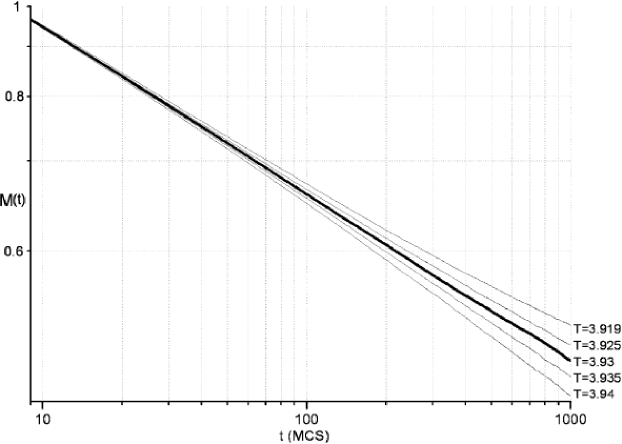
Figure 1: Time evolution of the magnetization $M(t)$ for $L=128$ and for different values of the temperature $T$.

The critical temperature determined in 5 for the same system with spin concentration $p=0.8$ in the non-Gaussian case is $T_{c}=3.8891(2)$. This difference of the critical temperature values shows that different principles of distribution of linear defects are the reason of discrepancy between the results obtained in 5 by Monte Carlo simulation of the 3D Ising model with LR-correlated disorder, and results in renormalization group description of this model 13 .

In order to check-up the critical temperature value independently, we have carried out in equilibrium the calculation of Binder cumulant $U_{4}$, defined as

$$U_{4}=\frac{1}{2}\left(3-\frac{[\left<M^{4}\right>]\phantom{{}^{2}}}{[\left<M^{2}\right>]^{2}}\right),$$ (13)

and the correlation length 28

$$\xi = \frac{1}{2\sin{(\pi/L)}}\sqrt{\frac{\chi}{F}-1\,},$$ (14)

$$\chi = \frac{1}{N_{spin}}[\langle M^{2}\rangle],$$ (15)

$$F = \frac{1}{N_{spin}}[\langle\Phi\rangle],$$ (16)

$$\Phi = \frac{1}{3}\sum_{n=1}^{3}\left(\left|\sum_{j}{p_{j}S_{j}\exp\left(\frac{2\pi ix_{n,j}}{L}\right)}\right|^{2}\right),$$ (17)

where $(x_{1,j},x_{2,j},x_{3,j})$ are coordinates of $j$-th site of lattice.

The cumulant $U_{4}(L,T)$ has a scaling form

$$U_{4}(L,T)=u\left(L^{1/\nu}(T-T_{c})\right).$$ (18)

The scaling dependence of the cumulant makes it possible to determine the critical temperature $T_{c}$ from the coordinate of the points of intersections of the curves specifying the temperature dependence $U_{4}(L,T)$ for different $L$. In Fig. 3a the computed curves of $U_{4}(L,T)$ are presented for lattices with sizes $L$ from 16 to 128. As a result it was determined that the critical temperature is $T_{c}=3.9275(5)$. In this case for simulations we have used the Wolff single-cluster algorithm with elementary MCS step as 5 cluster flips. We discard 10000 MCS for equilibration and then measure after every MCS with averaging over 100000 MCS. The results have been averaged over 15000 different samples for lattices with sizes $L=16,32$ and over 10000 samples for lattices with sizes $L=64,128$.

The crossing of $\xi/L$ was introduced as a convenient method for calculating of $T_{c}$ in 29 . In Fig. 3b the computed curves of temperature dependence of ratio $\xi/L$ are presented for lattices with the same sizes, the coordinate of the points of intersections of which also gives the critical temperature $T_{c}=3.9281(1)$. This value of $T_{c}$ we selected as the best for subsequent investigations of the Ising model.

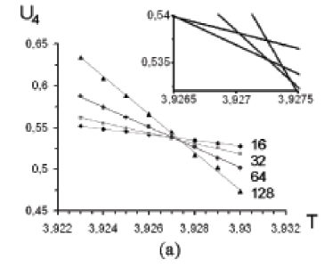
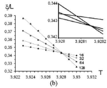
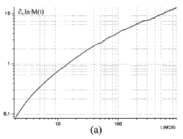
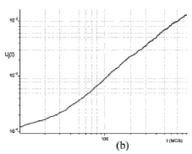
Figure 2: Binder cumulant $U_{4}(T,L)$ (a) and ratio $\xi/L$ (b) as a function of T for lattices with different sizes $L$.

Figure 3: Time evolution of logarithmic derivative of the magnetization $\left.\partial_{\tau}lnM(t,\tau)\right|_{\tau=0}$ (a) and the cumulant $U_{2}(t)$ (b) for $L=128$ at the critical temperature $T_{c}=3.9281$.

Also, we have determined the temperature of intersection of the curves specifying the temperature dependence cumulants $U_{4}(L,T)$ for $L=16$ and $L=32$ with the use of linear defects distribution in samples as in 5 with the possibility of their intersection. Computation gives $T_{c}(L)=3.8884(6)$ in this case which corresponds to the results in 5 but differs from $T_{c}(L)=3.9185(5)$ obtained with the use of condition of linear defects disjointness for lattices with the same sizes. Turning back to short-time dynamics method, we note that the exponent $1/\nu z$ can be determined from relation (9) if we differentiate $lnM(t,\tau)$ with respect to $\tau$.

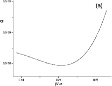
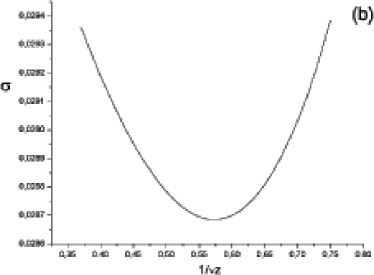
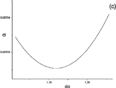
Figure 4: Dependence of the mean square errors $\sigma$ of the fits for the magnetization (a), logarifmic derivative of the magnetization (b), and the cumulant (c) as a function of the exponents $\beta/\nu z$, $1/\nu z$, and $d/z$ for $\omega=0.8$.

The dynamic exponent $z$ can be determined from analysis of time dependent Binder cumulant $U_{2}(t)$ (10) for $\tau=0$. In Fig. 3 the logarithmic derivative of the magnetization $\left.\partial_{\tau}lnM(t,\tau)\right|_{\tau=0}$ with respect to $\tau$ (Fig. 3a) and the cumulant $U_{2}(t)$ (Fig. 3b) for samples with linear size $L=128$ at $T_{c}=3.9281$ are plotted in log-log scale. The $\left.\partial_{\tau}lnM(t,\tau)\right|_{\tau=0}$ have been obtained from a quadratic interpolation between the three curves of time evolution of the magnetization for the temperatures $T=3.9250$, $3.9281$, $3.9310$ and taken at the critical temperature $T_{c}=3.9281$. The resulting curves have been obtained by averaging over 3000 samples.

We have analyzed the time dependence of the cumulant $U_{2}(t)$ and clarified that in the time interval [50,150] the $U_{2}(t)$ is best fitted by power law with the dynamic exponent $z\simeq 2.02$, corresponding to the pure Ising model 30 ; 31 , and the linear defects are developed for $t>400$ MCS only. An analysis of the $U_{2}(t)$ slope measured in the interval [500,900] shows that the exponent $d/z=1.173(12)$ which gives $z=2.558(26)$. We have taken into account these dynamic crossover effects for analysis of the time dependence of magnetization and its derivative. So, the slope of magnetization and its derivative over the interval [450,900] provides the exponets $\beta/\nu z=0.230(2)$ and $1/\nu z=0.517(12)$ which give $\nu=0.746(19)$ and $\beta=0.445(10)$.

In the next stage, we have considered the corrections to the scaling in order to obtain accurate values of the critical exponents. We have applied the following expression for the observable $X(t)$:

$$X(t)\sim t^{\Delta}\left(1+A_{x}t^{-\omega/z}\right),$$ (19)

where $\omega$ is a well-known exponent of corrections to scaling. This expression reflects the scaling transformation in the critical range of time-dependent corrections to scaling in the form of $t^{-\omega/z}$ to the usual form of corrections to scaling $\tau^{\omega\nu}$ in equilibrium state for time t comparable with the order parameter relaxation time $t_{r}\sim\xi^{z}\Omega(k\xi)$ 17 . Field-theoretic estimate of the $\omega$ value gives $\omega\simeq 0.80$ in the two-loop approximation 15 . Monte Carlo study of Ballesteros and Parisi 5 shows that $\omega\simeq 1.0$.

Table 1: Values of the exponents $\beta/\nu z$, $1/\nu z$, $d/z$, and minimal values of the mean square errors $\sigma$ in fits for different values of the exponent $\omega$

$\omega$	$\beta/\nu z$	$\sigma$	$1/\nu z$	$\sigma$	$d/z$	$\sigma$
0.7	0.2112	0.0100	0.556	0.0053	1.183	0.0100
0.8	0.2096	0.0088	0.559	0.0049	1.205	0.0100
0.9	0.2101	0.0093	0.553	0.0070	1.213	0.0099
1.0	0.2090	0.0095	0.558	0.0072	1.227	0.0098

To analyze our simulation date we have used the linear approximation of the $(Xt^{-\Delta})$ on $t^{-\omega/z}$ with the changing values of the exponent $\Delta$ and the exponent $\omega$ from the interval [0.7,1.0]. Then, we have investigated the dependence of the mean square errors $\sigma$ of this fitting procedure for the function $Xt^{-\Delta}(t^{-\omega/z})$ on the changing $\Delta$ and $\omega$. In Fig. 4 we plot the $\sigma$ for the magnetization (Fig. 4a), logarifmic derivative of the magnetization (Fig. 4b), and the cumulant (Fig. 4c) as a function of the exponents $\beta/\nu z$, $1/\nu z$, and $d/z$ for $\omega=0.8$. Minimum of $\sigma$ determines the exponents $z$, $\nu$, and $\beta$ for every $\omega$. In Table 1 we present the computed values of the exponents $\beta/\nu z$, $1/\nu z$, and $d/z$, and minimal values of the mean square errors $\sigma$ in these fits for values of the exponent $\omega=0.7,0.8,0.9,1.0$. We see that the values of $\beta/\nu z$, $1/\nu z$, and $d/z$ are weakly dependent on the change of the exponent $\omega$ in the interval [0.7,1.0], but the $\omega=0.8$ is preferable because it gives the best fit for the magnetization and the logarifmic derivative of the magnetization dates. Finally, for the $\omega=0.8$ we find the following values of the exponents

$$\begin{array}[]{rl}&z=2.489\pm 0.021,\\ &\nu=0.719\pm 0.022,\\ &\beta=0.375\pm 0.045.\end{array}$$ (20)

It is interesting to compare these values of exponents with those obtained in 13 with the use of the field-theoretic approach

$$\begin{array}[]{rl}&z=2.495,\\ &\nu=0.716,\\ &\beta=0.350,\end{array}$$ (21)

which demonstrate a very good agreement with each other, but show an essential difference from Monte Carlo results of Ballesteros and Parisi 5 with $\nu=1.009(13)$ and $\beta=0.526(15)$.

III.2 Evolution from a disordered state

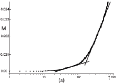
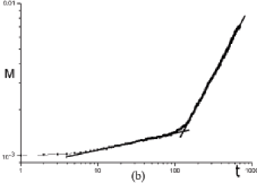
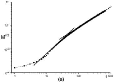
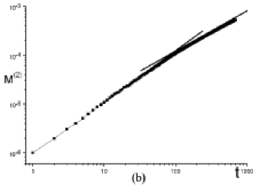
Figure 5: Time evolution of the magnetization $M(t)$ for $L=128$ with the initial magnetization $m_{0}=0.02$ (a) and $m_{0}=0.001$ (b) at the critical temperature $T_{c}=3.9281$.

Figure 6: Time evolution of the second moment $M^{(2)}$ for $L=128$ with the initial magnetization $m_{0}=0.02$ (a) and $m_{0}=0.001$ (b) at the critical temperature $T_{c}=3.9281$.

We have also performed simulations of evolution of the system with linear defects on the largest lattice with $L=128$, starting from a disordered state with small initial magnetizations $m_{0}=0.02$ and $m_{0}=0.001$ at the critical point. The initial magnetization has been prepared by flipping in an ordered state a definite number of spins at randomly chosen sites in order to get the desired small value of $m_{0}$. In accordance with Section II, a generalized dynamic scaling predicts in this case a power law evolution for the magnetization $M(t)$, the second moment $M^{(2)}(t)$ and the auto-correlation $A(t)$ in the short-dynamic region.

In Fig. 6, 6 and 7 we show the obtained curves for $M(t)$ (Fig. 6), $M^{(2)}(t)$ (Fig. 6) and $A(t)$ (Fig. 7), which are plotted in log-log scale up to $t=700$. These curves were resulted by averaging over 3000 different samples with 25 runs for each sample. From Fig. 6 we can see an initial increase of the magnetization, which is a very prominent phenomenon in the short-time critical dynamics 17 ; 18 . But in contrast to dynamics of the pure systems 17 , we can observe the crossover from dynamics of the pure system on early times of the magnetization evolution up to $t=70$ to dynamics of the disordered system with the influence of linear defects in the time interval [100,650].

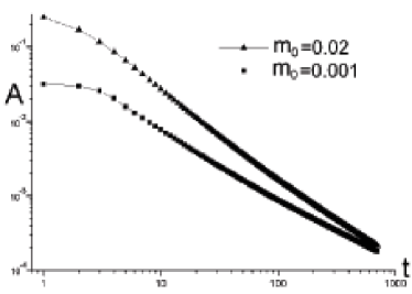
Figure 7: Time evolution of the autocorrelation $A(t)$ for $L=128$ with different initial magnetization values $m_{0}$ at the critical temperature $T_{c}=3.9281$.

The same crossover phenomena were observed in evolution of the second moment $M^{(2)}(t)$ and the autocorrelation $A(t)$. In result of linear approximation of these curves in the both time intervals we obtained the values of the exponents $\theta$, $c_{2}$ and $c_{a}$ in accordance with relations in (3), (5) and (6) for initial states with $m_{0}=0.02$ and $m_{0}=0.001$ (Table 2). The final values of these exponents and also the critical exponents $z$, $\beta/\nu$ and $x_{0}$ were obtained by extrapolation to $m_{0}=0$. In Table 2 we compare the values of these exponents with values of corresponding exponents for the pure Ising model 18 and theoretical field description (TFD) results for system with linear defects 13 . The obtained values quite well agree with results of simulation from an ordered state with $m_{0}=1$ and with results from 13 and show that LR-correlated defects lead to faster increasing of the magnetization in the short-time dynamic regime in compare with the pure system.

Table 2: Values of the critical exponents obtained in present work for evolution from disordered initial states with different $m_{0}$ and extrapolated to $m_{0}=0$ and corresponding exponents for pure systems 17 and from 13

	$\theta$	$c_{2}$	$c_{a}$	$z$	$\beta/\nu$	$x_{0}$
$t\in[10,70]$
$m_{0}=0,02$	0.086(12)	0.964(28)	1.384(26)
$m_{0}=0,001$	0.099(9)	0.973(19)	1.364(23)
$m_{0}=0$	0.101(10)	0.975(23)	1.363(26)	2.049(27)	0.501(27)	0.708(34)
$t\in[100,650]$
$m_{0}=0,02$	0.152(12)	0.812(21)	1.103(16)
$m_{0}=0,001$	0.149(10)	0.804(19)	1.047(12)
$m_{0}=0$	0.149(11)	0.801(20)	1.043(14)	2.517(32)	0.492(28)	0.867(37)
TFD 13				2.495	0.489
pure  17	0.108(2)	0.970(11)	1.362(19)	2.041(18)	0.510(14)	0.730(25)

III.3 Measurements of the critical characteristics in equilibrium state

With the aim to verify the short-time dynamics method and the results obtained we also carried out the study of the critical behavior of 3D Ising model with the linear defects of random orientation by traditional Monte Carlo simulation methods in equilibrium state. For simulations we have used the Wolf single-cluster algorithm. We have computed for the critical temperature $T_{c}=3.9281(1)$ the values of different thermodynamic and correlation functions in equilibrium state such as the magnetization, susceptibility, correlation length, heat capacity, and Binder cumulant $U_{4}$ for lattices with sizes $L$ from 16 to 128 for the same spin concentration $p=0.8$. The use of well-known scaling critical dependences for these thermodynamic and correlation functions with taking into consideration the finite size scaling corrections

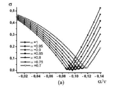
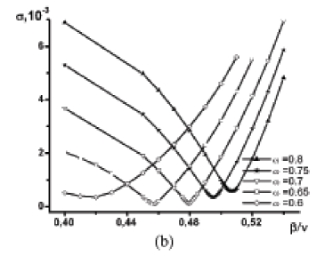
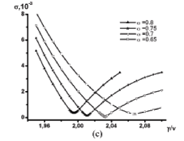
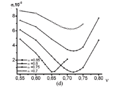
Figure 8: Dependence of the mean square errors $\sigma$ of the fits for heat capacity (a), magnetization (b), susceptibility (c), and thermal derivative of cumulant (d) as a function of the exponents $\alpha/\nu$, $\beta/\nu$, $\gamma/\nu$, and $\nu$ for different values of $\omega$.

$$C(L) \sim L^{\alpha/\nu}\left(1+aL^{-\omega}\right)$$ (22)

$$M(L) \sim L^{-\beta/\nu}\left(1+bL^{-\omega}\right)$$ (23)

$$\chi(L) \sim L^{\gamma/\nu}\left(1+cL^{-\omega}\right)$$ (24)

$$\frac{dU}{dT}(L) \sim L^{1/\nu}\left(1+dL^{-\omega}\right)$$ (25)

Table 3: Values of the exponents $\alpha/\nu$, $\beta/\nu$, $\gamma/\nu$, and $\nu$ with values of the exponent $\omega$, giving the best fit in approximation procedure

Table 4: Values of the critical exponents obtained in present work for average value of exponent $\omega=0.76$ and corresponding exponents from 13

	$\alpha/\nu$	$\beta/\nu$	$\gamma/\nu$	$\nu$
	$-0.096(3)$	$0.457(2)$	$2.032(1)$	$0.710(10)$
$\omega$	$0.90$	$0.65$	$0.70$	$0.80$

	$\alpha$	$\beta$	$\gamma$	$\nu$
present	$-0.078(30)$	$0.362(20)$	$1.441(15)$	$0.710(10)$
13	$-0.1048$	$0.3504$	$1.4453$	$0.7155$

makes it possible to determine the critical exponents $\alpha$, $\nu$, $\beta$, $\gamma$, and $\omega$ by means of statistical data processing of simulation results. To analyze simulation data we have used the linear approximation of the $(XL^{-\Delta})$ on $L^{-\omega}$ and then investigated the dependence of the mean square errors $\sigma$ of this fitting procedure for the function $XL^{-\Delta}(L^{-\omega})$ on the changing exponent $\Delta$ and $\omega$ values. In Fig. 8 we plot the $\sigma$ for heat capacity (Fig. 8a), magnetization (Fig. 8b), susceptibility (Fig. 8c), and temperature derivative of cumulant (Fig. 8d) as a function of the exponents $\alpha/\nu$, $\beta/\nu$, $\gamma/\nu$, and $\nu$ for different values of $\omega$. Minimum of $\sigma$ determines the values of exponents. In Table 4 we present the obtained values of the exponents $\alpha/\nu$, $\beta/\nu$, $\gamma/\nu$, $\nu$, and $\omega$, which give minimal values of $\sigma$ in these fits. Then we determine the average value of $\omega=0.76(5)$ with the use of which there were computed the final values of exponents. In Table 4 there are presented the values of the exponents obtained in this work by simulation methods and from 13 with the use of the field-theoretic approach and scaling relations for critical exponents.

The comparison these values shows their good agreement within the limits of statistical errors of simulation and numerical approximations and good agreement with the values of the static critical exponents computed by the short-time dynamics method.

IV Measurements of the critical temperature and critical exponents for 3D XY-model

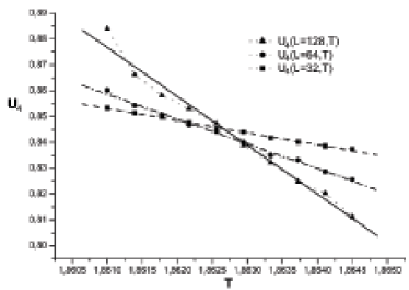
Figure 9: Binder cumulant $U_{4}(T,L)$ for 3D XY-model as a function of T for lattices with different sizes $L$.

Also, we have carried out the Monte Carlo study of the effect of LR-correlated quenched defects on the critical behavior of 3D XY-model characterized by the two-component order parameter. As is well-known 2 ; 13 , renormalization group analysis predicts the possibility of a new type of the critical behavior for this model different from the critical behavior of pure XY-like systems or systems with point-like uncorrelated defects. We considered the same site-diluted cubic lattices with linear defects of random orientation in the samples with the spin concentration $p=0.8$. The critical temperature $T_{c}=1.8626(5)$ was determined by the calculation of Binder cumulant $U_{4}(L,T)$ for lattices with sizes $L$ from 32 to 128 (Fig. 9). For simulations we have used the Wolff single-cluster algorithm.

IV.1 Evolution from an ordered state

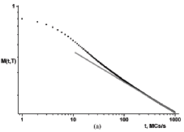
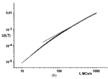
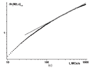
Figure 10: Time evolution of the magnetization $M(t)$ (a), Binder cumulant $U_{2}(t)$ (b) and the logarithmic derivative of the magnetization $\left.\partial_{\tau}lnM(t,\tau)\right|_{\tau=0}$ (c) for 3D XY-model with lattice size $L=128$ at the critical temperature $T_{c}=1.8626$.

We have performed simulations of the critical relaxation of the XY-model with linear defects starting from an ordered initial state. As example, in Fig. 10 we show the obtained curves for the magnetization $M(t)$ (Fig. 10a), Binder cumulant $U_{2}(t)$ (Fig. 10b) and the logarithmic derivative of the magnetization $\left.\partial_{\tau}lnM(t,\tau)\right|_{\tau=0}$ (Fig. 10c), which are plotted in log-log scale up to $t=1000$ for lattices with $L=128$. These curves were resulted by averaging over 3000 different samples. On these figures we can observe the crossover from dynamics, which is similar to that in the pure system on early times of the evolution up to $t=150$, to dynamics of the disordered system with the influence of linear defects in the time interval [350,800]. The slope of $M(t)$, $U_{2}(t)$ and $\left.\partial_{\tau}lnM(t,\tau)\right|_{\tau=0}$ over the interval [350,800] provides the exponents $\beta/\nu z=0.239(1)$, $d/z=1.221(21)$ and $1/\nu z=0.531(13)$, whereas our theoretical-field predictions 13 give the following values of exponents $\beta/\nu z=0.204$, $d/z=1.268$ and $1/\nu z=0.556$. As well as for Ising model, we have considered the corrections to the scaling in order to obtain accurate values of the critical exponents in concordance with procedure, which was discussed in Subsection III.1.

As a result of this analysis we obtained the following values of critical exponents

$$\begin{array}[]{rl}&z=2.364\pm 0.007,\\ &\nu=0.778\pm 0.026,\\ &\beta=0.370\pm 0.030,\\ &\omega=1.05\pm 0.04.\end{array}$$ (26)

The comparison of these values of exponents with those obtained in 13 with the use of the field-theoretic approach $z=2.365$, $\nu=0.760$, $\beta=0.366$, and $\omega=1.15$ in 15 shows their good agreement within the limits of statistical errors of simulation and numerical approximations.

The obtained results confirm the strong effect of LR-correlated quenched defects on both the critical behavior of 3D Ising model and the systems characterized by the many-component order parameter.

IV.2 Evolution from a disordered state

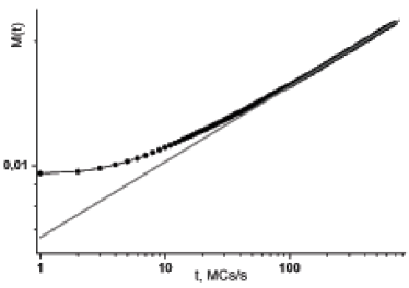
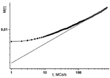
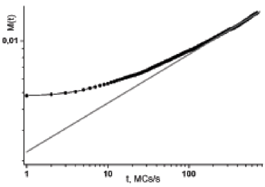
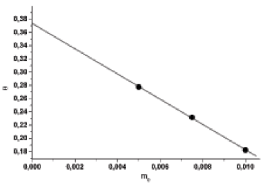
Figure 11: Time evolution of the magnetization $M(t)$ for 3D XY-model with the initial magnetization $m_{0}=0.01$ (a), $m_{0}=0.0075$ (b) and $m_{0}=0.005$ (c) at the critical temperature $T_{c}=1.8626$; determination of asymptotic value of the dynamic critical exponent $\theta$ in the limit $m_{0}\to 0$ (d).

We have also performed simulations of evolution of the system with linear defects on the largest lattice with $L=128$, starting from a disordered state with small initial magnetizations $m_{0}=0.01$, $m_{0}=0.0075$ and $m_{0}=0.005$ at the critical point. The initial magnetization has been prepared by flipping in an ordered state a definite number of spins at randomly chosen sites in order to get the desired small value of $m_{0}$. In accordance with Section II, a generalized dynamic scaling predicts in this case a power law evolution for the magnetization $M(t)$, the second moment $M^{(2)}(t)$ and the auto-correlation $A(t)$ in the short-dynamic region.

In Fig. 11 and 12 we show the obtained curves for $M(t)$ (Fig. 11), $M^{(2)}(t)$ and $A(t)$ (Fig. 12), which are plotted in log-log scale up to $t=700$. These curves were resulted by averaging over 3000 different samples with 25 runs for each sample. From Fig. 11 we can see also an initial increase of the magnetization, which is a very prominent phenomenon in the short-time critical dynamics. But in contrast to dynamics of the pure systems, we can observe, as previously for Ising model, the crossover from dynamics of the pure system on early times of the magnetization evolution up to $t=100$ to dynamics of the disordered system with the influence of linear defects in the time interval [200,650]. In this time interval we determined the values of the dynamic critical exponent $\theta$, which are equal $\theta=0.182(3)$ for case with the initial magnetization $m_{0}=0.01$, $\theta=0.232(7)$ for $m_{0}=0.0075$ and $\theta=0.278(11)$ for $m_{0}=0.005$. Then, in accordance with (3) the asymptotic value of the exponent $\theta=0.374(14)$ was determined in the limit $m_{0}\to 0$ (Fig. 11d) with the use of linear extrapolation.

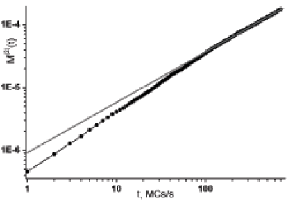
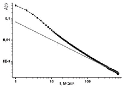
Figure 12: Time evolution of the second moment $M^{(2)}$ (a) and the auto-correlation $A(t)$ (b) for 3D XY-model with the initial magnetization $m_{0}=0$ at the critical temperature $T_{c}=1.8626$.

The analysis of results for evolution of the second moment $M^{(2)}(t)$ (Fig. 12a) and the autocorrelation $A(t)$ (Fig. 12b), obtained for simulation of systems with the initial magnetization $m_{0}=0$ (in reality for $m_{0}=10^{-6}$ such as for XY-model the spin configuration with $m_{0}=0$ is impossible to prepare), gives directly the values of exponents $c_{2}=0.825(23)$ and $c_{a}=0.907(30)$ for the time interval [300,650]. The same crossover phenomena is observed in evolution of $M^{(2)}(t)$ and $A(t)$ from dynamics of the pure system on early times to dynamics of the disordered system with the influence of linear defects.

On basis of these values of exponents $\theta$, $c_{2}$ and $c_{a}$ we obtained the exponents $z=2.342(57)$ and $\beta/\nu=0.534(35)$, which quite well agree with results of simulation from an ordered initial state with $m_{0}=1$ and with results of theoretical field description for XY-like systems with linear defects 13 within the limits of statistical errors of simulation and numerical approximations.

V Conclusion remarks

The present results of Monte Carlo investigations allow us to recognize that the short-time dynamics method is reliable for the study of the critical behavior of the systems with quenched disorder and is the alternative to traditional Monte Carlo methods. But in contrast to studies of the critical behavior of the pure systems by the short-time dynamics method, in case of the systems with quenched disorder corresponding to randomly distributed linear defects after the microscopic time $t_{mic}\simeq 10$ there exist three stages of dynamic evolution. For systems starting from the ordered initial states ($m_{0}=1$) in the time interval of 50-200 MCS, the power-law dependences are observed in the critical point for the magnetization $M(t)$, the logarithmic derivative of the magnetization $\left.\partial_{\tau}lnM(t,\tau)\right|_{\tau=0}$ and Binder cumulant $U_{2}(t)$, which are similar to that in the pure system. In the time interval [450,900], the power-law dependences are observed in the critical point which are determined by the influence of disorder. However, careful analysis of the slopes for $M(t)$, $\left.\partial_{\tau}lnM(t,\tau)\right|_{\tau=0}$ and $U_{2}(t)$ reveals that a correction to scaling should be considered in order to obtain accurate results. The dynamic and static critical exponents were computed with the use of the corrections to scaling for the Ising and XY models with linear defects, which demonstrate their good agreement with results of the field-theoretic description of the critical behavior of these models with long-range correlated disorder. In intermediate time interval of 200-400 MCS the dynamic crossover behavior is observed from the critical behavior typical for the pure systems to behavior determined by the influence of disorder.

The investigation of the critical behavior of the Ising model with extended defects starting from the disordered initial states with $m_{0}\simeq 0$ also have revealed three stages of the dynamic evolution. It was shown that the power-law dependences for the magnetization $M(t)$, the second moment $M^{(2)}(t)$ and the autocorrelation $A(t)$ are observed in the critical point, which are typical for the pure system in the interval [10,70] and for the disordered system in the interval [100,650]. In intermediate time interval the crossover behavior is observed in the dynamic evolution of the system. The obtained values of exponents demonstrate a good agreement within the limits of statistical errors of simulation and numerical approximations with results of simulation of the pure Ising model by the short-time dynamics method 13 for the first time interval and with our results of simulation of the critical relaxation of this model from the ordered initial states.

Also, we would like to note that over complicated critical dynamics of the systems with quenched disorder the accurate determination of the critical temperature is better to carry out in equilibrium state from the coordinate of the points of intersections of the curves specifying the temperature dependence of Binder cumulants $U_{4}(L,T)$ or ratio $\xi/L$ for different linear sizes $L$ of lattices.

The obtained results for 3D XY-model confirm the strong influence of LR-correlated quenched defects on the critical behavior of the systems described by the many-component order parameter. As a result, a wider class of disordered systems, not only the three-dimensional Ising model, can be characterized by a new type of critical behavior induced by quenched disorder.

We are planning to continue the Monte Carlo study of critical behavior of the model with LR-disorder for different spin concentrations $p$ and investigate the universality of critical behavior of diluted systems with LR-disorder focusing on the problem of disorder independence of asymptotic characteristics.

References

- (1) R. Folk, Yu. Holovatch and T. Yavors’kii, Phys. Usp. 46 (2003), 169 [Uspekhi Fiz. Nauk 173 (2003), 175].
- (2) A. Weinrib and B.I. Halperin, Phys. Rev. B 27, (1983), 413.
- (3) A.B. Harris, J. Phys. C: Solid State Phys. 7 (1974), 1671.
- (4) A.L. Korzhenevskii, A.A. Luzhkov and W. Schirmacher, Phys. Rev. B 50, (1998), 3661.
- (5) H.G. Ballesteros and G. Parisi, Phys. Rev. B 60, (1999), 912.
- (6) G. Jug, Phys. Rev. B 27, (1983), 609.
- (7) I.O. Mayer, J. Phys. A: Math. Gen. 22 (1989), 2815.
- (8) V.V. Prudnikov, S.V. Belim, A.V. Ivanov, E.V. Osintsev and A.A. Fedorenko, Sov. Phys.–JETP 87 (1998), 527
- (9) V.V. Prudnikov, P.V. Prudnikov and A.A. Fedorenko, Sov. Phys.–JETP Lett. 68 (1998), 950.
- (10) S.N. Dorogovtsev, J. Phys. A: Math. Gen. 17 (1984), L677.
- (11) E. Korucheva and D. Uzunov, Phys. Status Solidi (b) 126 (1984), K19.
- (12) E. Korucheva and F.J. De La Rubia, Phys. Rev. B 58, (1998), 5153.
- (13) V.V. Prudnikov, P.V. Prudnikov and A.A. Fedorenko, Phys. Rev. B 62, (2000), 8777.
- (14) K. Binder and J.D. Regir, Adv. Phys. 41 (1992), 547.
- (15) V. Blavats’ka, C. von Ferber and Yu. Holovatch, Phys. Rev. E 64, (2001), 041102.
- (16) M. Altarelli, M.D. Nunez-Regueiro and M. Papoular, Phys. Rev. Lett. 74, (1995), 3840.
- (17) B. Zheng, Int. J. Mod. Phys. B 12 (1998), 1419.
- (18) A. Jaster, J. Mainville, L. Schulke and B. Zheng, J. Phys. A 32 (1999), 1395.
- (19) P.C. Hohenberg and B.I. Halperin, Rev. Mod. Phys. 49 (1977), 435.
- (20) H.K. Janssen, B. Schaub and B. Schmittmann, Z. Phys. B 73 (1989), 539.
- (21) D. Huse, Phys. Rev. B 40, (1989), 304.
- (22) B. Zheng, Physica A 283 (2000), 80.
- (23) H.K. Janssen, From Phase Transitions to Chaos, edited by G.Gyorgyi, I.Kondor, L.Sasvari, and T.Tel, Topics in Modern Statistical Physics (World Scientific, Singapore, 1992).
- (24) N. Ito, Physica A 192 (1993), 604.
- (25) Y. Ozeki and N. Ito, Phys. Rev. B 64, (2001), 024416.
- (26) Y. Ozeki, K. Ogawa and N. Ito, Phys. Rev. E 67, (2003), 026702.
- (27) Y. Ozeki and N. Ito, Phys. Rev. B 68, (2003), 054414.
- (28) F. Cooper, B. Freedman and D. Preston, Nucl. Phys. B 210, (1989), 210.
- (29) H.G. Ballesteros, L.A. Fernández, V. Martín-Mayor and A. Muñoz Sudupe, Phys. Lett. B 378 (1996), 207; Phys. Lett. B 387 (1996), 125; Nucl. Phys. B 483, (1997), 707.
- (30) U. Krey, Z. Phys. B 26 (1977), 355.
- (31) V.V. Prudnikov, A.V. Ivanov and A.A. Fedorenko, Sov. Phys.–JETP Lett. 66 (1997), 835.