Measuring AGN Feedback with the Sunyaev-Zel’dovich Effect

Abstract

One of the most important and poorly-understood issues in structure formation is the role of outflows driven by active galactic nuclei (AGN). Using large-scale cosmological simulations, we compute the impact of such outflows on the small-scale distribution of the cosmic microwave background (CMB). Like gravitationally-heated structures, AGN outflows induce CMB distortions both through thermal motions and peculiar velocities, by processes known as the thermal and kinetic Sunyaev-Zel’dovich (SZ) effects, respectively. For AGN outflows the thermal SZ effect is dominant, doubling the angular power spectrum on arcminute scales. But the most distinct imprint of AGN feedback is a substantial increase in the thermal SZ distortions around elliptical galaxies, post-starburst ellipticals, and quasars, which is linearly proportional to the outflow energy. While point source subtraction is difficult for quasars, we show that by appropriately stacking microwave measurements around early type galaxies, the new generation of small-scale microwave telescopes will be able to directly measure AGN feedback at the level important for current theoretical models.

1. Introduction

Large-scale measurements of cosmic microwave background (CMB) anisotropies have played a central role in the development of the modern cosmological model. By giving us a picture of the universe during the epoch of linear fluctuations, they have provided us with a foundation from which to interpret the subsequent growth of structure. Thus from the spectacular initial detections made by the COBE satellite (Smoot et al. 1992), to the detailed flatness constraints provided by balloon-born missions (Hanany et al. 2000; Mauskopf et al. 2000), to the precision measurements of cosmological parameters derived from the WMAP observations (Spergel et al. 2003; 2007), our understanding of structure formation has progressed hand-in-hand with improvements in large-scale CMB anisotropy measurements.

On angular scales below $\approx 10^{\prime},$ the science potential of CMB measurements has yet to be realized. On these scales, Silk damping washes out the primary anisotropies, while a host of smaller-scale secondary anisotropies are imprinted as the photons propagate across the universe. One of the most important sources of these effects is the scattering of CMB photons by hot electrons, a process that was first studied by Sunyaev & Zel’dovich (1970; 1972). This process can be divided into two contributions. The largest of these is the thermal Sunyaev-Zel’dovich (SZ) effect in which inverse Compton scattering preferentially increases the energy of CMB photons passing through hot and dense regions, introducing anisotropies with a distinctive frequency dependence. A smaller contribution arises from the kinetic SZ effect in which Doppler scattering in dense regions with significant peculiar motions induces fluctuations with the same frequency dependence as the CMB itself.

The most important source of such hot and dense regions is undoubtedly the gravitational collapse of gas into large dark matter halos, and numerous numerical simulations of the Sunyaev-Zel’dovich effect from this process have been carried out by several groups (e.g. Scaramella, Cen, & Ostriker 1993; Hobson & Magueijo 1996; da Dilva et al. 2000; Refregier et al. 2000; Seljak, Burwell, & Pen 2001; Springel, White, & Hernquist 2001; Zhang, Pen, & Wang 2002; Roncarelli et al. 2007). Yet dark-matter driven gravitational heating need not provide the dominant SZ contribution at all scales and in all environments. In fact the gas responsible for the largest SZ distortions, the intracluster medium (ICM) in galaxy clusters, is observed to have been substantially heated by nongravitational sources (Cavaliere et al. 1998; Kravtsov & Yepes 2000; Wu et al. 2000; Babul et al. 2002). In galaxy groups, such nongravitational effects are even more severe, causing groups with a large range of X-ray luminosities to all be heated to a similar value of $\approx 1$ keV per baryon (e.g. Arnaud & Evrard 1999; Helsdon & Ponman 2000).

But perhaps the most dramatic, yet poorly understood manifestation of nongravitational heating is in establishing the observed “downsizing” (Cowie et al. 1996) trend in the evolution of star-forming galaxies and active galactic nuclei (AGN). Here the issue is that since $z\approx 2$ the characteristic mass scale of star-forming galaxies and the typical luminosities of AGN have dropped by over an order of magnitude (e.g. Arnouts et al. 2005, Treu et al. 2005; Pei 1995; Ueda et al. 2003; Barger et al. 2005). This “antiheirarchical” trend is in direct conflict with the expectations of the long-standing model of structure formation in which gas condensation and heating is driven purely by dark mater halos, which grow hierarchically by accretion and merging over time. In this picture, as gas falls into potential wells, it is shock heated and must radiate this energy away before forming stars (Rees & Ostriker 1977; Silk 1977). The larger the structure, the longer it takes to cool, and thus the formation of history of galaxies is even more hierarchical than the dark matter history.

Although early modeling did not reproduce this downsizing behavior, the trend has been successfully reproduced in more recent theoretical models that include a large source of heating associated with outflows from AGN (Scannapieco & Oh 2004; Binney 2004; Granato et al. 2004; Scannapieco, Silk, & Bouwens 2005; Di Matteo, Springel, & Hernquist 2005; Croton et al. 2006; Cattaneo et al. 2006; Thacker, Scannapieco, & Couchman 2006, hereafter TSC06; Di Matteo et al. 2007). In this picture, AGN outflows associated with broad-absorption line winds and radio jets heat the surrounding intergalactic medium (IGM) to sufficiently high temperatures to prevent it from cooling and thus from forming further generations of stars and AGN. This feedback requires an energetic outflow, driven by a large AGN, to be effective in the dense, high-redshift IGM, while in the more tenuous low-redshift IGM, equivalently long cooling times can be achieved by less energetic winds. The lower the redshift, the smaller the galaxy that is able to exert efficient feedback, thus resulting in cosmic downsizing.

However, the details of AGN feedback remain extremely uncertain. Heating may be impulsive (e.g. TSC06), more gradual (e.g. Brüggen, Ruszkowski, & Hallman 2005; Croton et al. 2006), or modulated primarily by the properties of the surrounding material (e.g. Dekel & Birnboim 2006). Furthermore, direct measurements of the kinetic energy input from AGN are notoriously difficult and range from $\sim 1\%$ or less (de Kool 2001) to $\sim 60\%$ of the AGN’s total bolometric energy (Chartas et al. 2007). Finally, several alternative ideas have been suggested to explain downsizing outside of the context of AGN feedback altogether (e.g. Kereš, et al. 2005; Khochhfar & Ostriker 2007; Birnboim, Dekel, & Neistein 2007).

Here we show that the definitive measurement resolving this issue may again come from the microwave background, through observations of SZ distortions. As it directly probes the spatial distribution of heated gas, SZ detections are able to place constraints on the primary theoretical uncertainty in AGN feedback models, namely the nature and degree of nongravitational gas heating. Fortunately, the rise in importance of this issue for theory is paralleled by recent advances in observation. Motivated primarily by deriving cosmological constraints though the detection of galaxy clusters (e.g. Holder et al. 2000; Majumdar & Mohr 2003; Battye & Weller 2003; Schulz & White 2003), a large number of blank-field small-scale CMB surveys are now underway, using telescopes that will push into the interesting regime for AGN feedback. These include surveys with the Atacama Cosmology Telescope (Kosowsky et al. 2006), the South Pole Telescope (Ruhl et al. 2004), the Atacama Pathfinder Experiment (Dobbs et al. 2006), and the Sunyaev-Zel’dovich Array (Loh et al. 2005), many of which will be coordinated to overlap with optical surveys. These advances are particularly important as less sensitive small-scale CMB surveys have already hinted at an excess of SZ distortions (Mason et al. 2003; Bond 2005; Dawson et al. 2006; Kuo et al. 2007).

In this work we make use of the first large-scale cosmological hydrodynamical simulation to explicitly include AGN feedback (TSC06) to construct detailed maps of their imprint on the CMB. Analyzing these maps and comparing them with other observables, we are able to determine the most promising approaches to using these ongoing surveys to constrain AGN feedback. Previous studies of nongravitational heating on the SZ background focused on the impact of starburst winds at high redshift (Majumdar, Nath, & Chiba 2001; White, Hernquist, & Springel 2002) and signatures from Population III stars (Oh, Cooray,& Kamionkowski 2003). Recently, Chatterjee & Kosowsky (2007) made analytic estimates of the impact of quasar winds on the CMB power spectrum and the cross-correlation of the SZ effect with optical sources. Here we show directly from simulations that while basic quantifiers such as the power spectrum are difficult to interpret, approaches based on the cross-correlation of SZ distortions with optical observations will soon provide a clean and direct probe of AGN feedback.

The structure of this work is as follows. In §2 we describe our numerical simulations and the methods used to construct maps of the CMB distortions from the kinetic and thermal SZ effects. In §3 we compute the contribution of AGN outflows to the CMB power spectrum, calculate their impact on the regions surrounding individual galaxies and AGN, and quantify the sensitivity of CMB-galaxy cross correlations to AGN feedback. Finally, our conclusions are summarized in §4.

2. Method

2.1. Simulations

In order to disentangle the SZ signatures of AGN feedback from distortions due purely to gravitational heating, we made use of two simulations, the large AGN feedback simulation first presented in TSC06 (using $2\times 640^{3}$ particles) and a smaller-scale comparison simulation (using $2\times 320^{3}$ particles) in which structure formation, gas cooling, and star formation were tracked exactly as in the fiducial run but no outflows were added. In both cases, based on wide range of cosmological constraints (e.g. Spergel et al. 2003; Vianna & Liddle 1996; Riess et al. 1998; Perlmutter et al. 1999), we adopted Cold Dark Matter cosmological model with parameters $h=0.7$, $\Omega_{0}$ = 0.3, $\Omega_{\Lambda}$ = 0.7, $\Omega_{b}=0.046$, $\sigma_{8}=0.9$, and $n=1$, where $h$ is the Hubble constant in units of 100 km s^-1 Mpc^-1, $\Omega_{0}$, $\Omega_{\Lambda}$, and $\Omega_{b}$ are the total matter, vacuum, and baryonic densities in units of the critical density, $\sigma_{8}^{2}$ is the variance of linear fluctuations on the $8h^{-1}{\rm Mpc}$ scale, and $n$ is the “tilt” of the primordial power spectrum. Note that these parameters are slightly different than those preferred by the more recent WMAP data (Spergel et al. 2007), which was released after our large AGN feedback run had already been completed. Initial conditions were computed using the Eisenstein & Hu (1999) transfer function.

In both runs, as in our previous work (e.g. Scannapieco, Thacker, & Davis 2001), simulations were conducted with a parallel OpenMP based implementation of the “HYDRA” code (Thacker & Couchman 2006) that uses the Adaptive Particle-Particle, Particle-Mesh algorithm to calculate gravitational forces (Couchman 1991), and the smooth particle hydrodynamic (SPH) method to calculate gas forces (Lucy 1977; Gingold & Monaghan 1977). As the details of this code and our outflow implementation are described in detail elsewhere (Scannapieco, Thacker, & Davis 2001; TSC06) here we only summarize the aspects most relevant to the SZ effect.

Our study is targeted to relatively large and late forming structures, and for both runs we have kept the metallicity constant at $Z=0.05$, to mimic a moderate level of enrichment. Similarly, because the epoch of reionization is poorly known and because reionization has little impact on mass scales greater than $10^{9}$$\rm\thinspace M_{\odot}$(Barkana, & Loeb 1999), we did not include a photoionization background in either simulation. In our AGN feedback run, which was designed to cover a large range in the AGN luminosity function, we used a simulation box of size $146h^{-1}$ Mpc filled with $2\times 640^{3}$ particles, which corresponded to a dark-matter particle mass of $1.9\times 10^{8}{M_{\odot}}$ and a gas particle mass of $2.7\times 10^{7}{M_{\odot}}.$ Our comparison simulation, which was carried out purely for the purposes of the current study, used $320^{3}$ particles in a box $73h^{-1}$ comoving Mpc on a side, corresponding to the same particle masses as in the AGN run. Both runs were terminated at $z=1.2$, at which point integration was becoming expensive due to the single-stepping nature of the Hydra code, and impractical in a shared queue environment. This means that our results do not contain the SZ contribution from lower redshifts, during which most galaxy clusters are formed. However, as $z=1.2$ is well past the peak epoch of AGN activity (eg. Ueda et al. 2003; Barger et al. 2005), our results should do well at quantifying the AGN contribution to the SZ effect, which is our main focus here.

As in TSC06, bright quasar-phase AGN are associated with galaxy mergers, which are tracked by labeling gas particles and identifying new groups in which at least 30% of the accreted mass does not come from a single massive progenitor. Once a merger has been identified, we compute the mass of the associated supermassive black hole, $M_{\rm BH},$ from the circular velocity of the remnant, $v_{\rm c}$ using the observed $M_{\rm BH}-v_{\rm c}$ relation (Merrit & Ferrarese 2001; Tremaine et al. 2001; Ferrarese 2002) which gives

$$M_{\rm BH}=2.8\times 10^{8}\left(\frac{v_{\rm c}}{300\,{\rm km}\,{\rm s^{-1}}}\right)^{5}.$$ (1)

Here $v_{\rm c}$ is estimated as

$$v_{\rm c}=\left[\frac{4\pi}{3}G\rho_{\rm v}(z)r_{\rm v}^{2}\right]^{1/2},$$ (2)

where $G$ is the gravitational constant, $\rho_{\rm v}(z)$ is the virial density as a function of redshift, and $r_{\rm v}$ is the implied virial radius for a group of $N$ gas particles with mass $m_{\rm g}$

$$r_{\rm v}=\left[{Nm_{\rm g}\Omega_{0}/\Omega_{b}\over 4/3\pi\rho_{\rm v}(z)}\right]^{1/3}.$$ (3)

Following Wyithe & Loeb (2002) and Scannapieco & Oh (2004), we assume that for each merger the accreting black hole shines at its Eddington luminosity ($1.2\times 10^{38}$ ergs s^-1 ${M_{\odot}}^{-1}$) for a time taken to be a fixed fraction of the dynamical time of the system, $t_{\rm d}=0.055r_{\rm v}/v_{\rm c}=5.8\times 10^{-3}\Omega(z)^{-1/2}H(z)^{-1}$. In TSC06 it was demonstrated that, apart from a discrepancy for the very luminous end, this simple model does extremely well at reproducing the observed AGN luminosity function as well as the large and small-scale clustering of AGN over the full range of simulated redshifts. Furthermore, the discrepancy at the very luminous end for the simulation as compared to the semi-analytic model could be attributed to the relative efficiency of shock heating on substructure (e.g. see Agertz et al. 2006 for a discussion of numerical ”stripping” issues). Note that while our approach does not distinguish between AGN formed in gas-rich “wet” mergers and gas-poor “dry” mergers, unlike at lower redshift (e.g. Bell et al. 2006), dry mergers are likely to be relatively unimportant at the $z\geq 1.2$ redshifts we are studying.

In our fiducial run, we also assume that a fixed fraction $\epsilon_{\rm k}=0.05$ of the bolometric energy of each AGN is channeled into a kinetic outflow. This value is consistent with other literature estimates (e.g. Furlanetto & Loeb 2001; Nath & Roychowdhury 2002), as well as observations (Chartas et al. 2007). Each outflow is then launched with an energy input of

$$E_{\rm k}=6\times 10^{36}\;\left({M_{\rm bh}\over\hbox{$\rm\thinspace M_{\odot}$}}\right)\left({t_{\rm d}\over{\rm s}}\right)\;{\rm ergs}.$$ (4)

Given the uncertainties surrounding AGN outflows, we simply model each expanding outflow as a spherical shell at a radius $2r_{\rm v}$ which is constructed by rearranging all the gas within this radius, but outside $r_{\rm v},$ and below a density threshold of $2.5\rho_{\rm v}.$ Finally, the radial velocity $v_{s}$ and temperature $T_{s}$ of the shell are determined by fixing the postshock temperature, $T_{s}$, to be $T_{s}=13.6K[v_{s}/({\rm km}{\rm s}^{-1})]^{2}$ and choosing $v_{s}$ such that the sum of the thermal and kinetic energy of the shell equals $E_{\rm k}$ minus the energy used to move particles from their initial positions into the shell. As shown in TSC06, this prescription results in a level of preheating in galaxy clusters and groups that is in good agreement with observations.

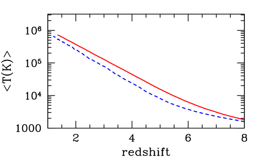
Figure 1.— Evolution of the mass-averaged gas temperature in our AGN feedback (solid) and comparison (dashed) runs.

In Figure 1, we show the mass-averaged gas temperature in our AGN feedback and comparison runs. The presence of outflows has a substantial impact on the IGM, raising the mean gas temperature in the simulation by $\approx 50\%$. Furthermore, as discussed in TSC06, most of this heating is targeted toward the densest regions, exactly those that contribute most to the SZ effect.

2.2. Construction of SZ maps

As the thermal and kinetic SZ effect have different frequency distributions, we calculate each of them separately from our simulations. In the (nonrelativistic) thermal SZ case, the change in the temperature of the CMB as a function of frequency is given by

$$\frac{\Delta T}{T}=y\left[x\frac{e^{x}+1}{e^{x}-1}-4\right],$$ (5)

where $x=h\nu/kT_{\rm CMB}$ is the dimensionless frequency, and the Compton $y$ parameter is defined as

$$y\equiv\sigma_{T}\int dl\,n_{e}\frac{k(T_{e}-T_{\rm CMB})}{m_{e}c^{2}},$$ (6)

where $\sigma_{T}$ is the Thompson cross section, $m_{e}$ is the mass of the electron, $n_{e}$ is the density of electrons, $T_{e}$ is the electron temperature, $T_{\rm CMB}$ is again the temperature of the CMB, and the integral is performed over the proper distance along the line of sight. Note that $y$ is simply a rescaled version of the line-of-sight integral of the pressure. Note also that in the Rayleigh-Jeans limit, in which $x\ll 1,$ eq. (5) reduces to $-2y,$ and we focus on this limit throughout our discussion below.

For the kinetic SZ effect, on the other hand, the magnitude of the CMB distortions is frequency independent and $\Delta T/T=-b$. In this case

$$b\equiv\sigma_{T}\int dl\,n_{e}\frac{v_{r}}{c},$$ (7)

where $v_{r}$ is the radial peculiar velocity of the gas, and the integral is again performed along the line of sight.

To construct maps of these distortions from our simulations, we followed a method similar to da Silva et al. (2000) and Springel et al. (2002). For each simulation output, we smoothed the density, temperature, and velocity fields onto a cubic grid. The smoothing procedure used the standard SPH smoothing methodology, that cells at a distance $|{\bf r}_{cell}-{\bf r}_{i}|$ from a particle $i$, are incremented by

$$A_{cell}\equiv{1\over w_{n_{i}}}{A_{i}\over\rho_{i}}m_{i}W(|{\bf r}_{cell}-{\bf r}_{i}|,h_{i}),$$ (8)

where $A_{i}$ is the scalar field value for particle $i$, $\rho_{i}$ is the density of particle $i$, $W$ is the B2-spline kernel, and $w_{n_{i}}$ is a normalization factor. The smoothing process generalizes in the natural fashion for vector fields. The normalization factor is required to ensure that the weighting of the assigned kernel is correct when summed across a finite number of cells (the standard kernel definition normalizes to unity over a continuous spherical volume of radius $2h_{i}$). If a particle is smoothed over $n_{cell}$ cells within a spherical volume specified by the radius $2h_{i}$, then $w_{n_{i}}$ is given by

$$w_{n_{i}}=\sum_{k=1}^{n_{cell}}W(|{\bf r}_{cell_{k}}-{\bf r}_{i}|,h_{i}),$$ (9)

where we have used $k$ to distinguish that the summation is over cells, rather than over particles.

Once the smoothed grid had been constructed it was then projected in the $x$, $y$ and $z$ directions. Since projection amounts to a summation along each axis direction the smoothing process could potentially have been performed in two dimensions alone. However, we project the three dimensional grid to ensure that the integration in the projection axis accounted for the quantization effects associated with smoothing onto a fixed number of cells. Next we constructed a grid of spanning ($1.1$ deg)² and made up of 1024² rays in the fiducial run, and spanning ($0.55$ deg)² and made up of 512² rays in the comparison run, such that in both cases the full simulation subtended an angle equal to the field at our highest redshift output of $z=10.$ Finally we projected along each of our sightlines, choosing a random translation and orientation at every redshift, and weighting the slices according to eqs. (6) and (7).

3. Results

3.1. Overall Properties

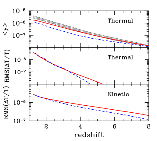
Figure 2.— Top: Total integrated value of the evolution of the average Compton $y$ parameter as a function of redshift for the AGN feedback run (solid line) and comparison run (dashed line) The shaded region is bounded below by the Scannapieco & Oh (2004) predictions for the $y$ distortion due to AGN feedback (with $\epsilon_{k}=0.05$) and from above by the sum of this prediction plus the results of our comparison run. Middle: Total RMS value of $\Delta T/T=-2y$ from the thermal SZ effect, as a function of redshift, with lines as in the upper panel. Bottom: Total RMS $\Delta T/T$ from the kinetic SZ effect as a function of redshift.

In Figure 2, we study which redshifts contribute most to CMB distortions, by integrating from $z=10$ (our assumed redshift of reionization) down to various redshifts. From eq. (6) the change in the average Compton $y$ distortion per unit $dl$ is proportional to the mass-average temperature. Thus, consistent with the temperature evolution shown in Figure 1, $\left<y\right>$ is roughly $50\%$ higher in the AGN feedback run at all redshifts. Furthermore, for most redshifts, this increase is similar to the one derived from analytic estimates as presented in Scannapieco & Oh (2004). In fact, the difference between this model and our simulations may be due to the presence of small-scale structure around AGN outflows, which were ignored in the analytic estimates, and whose mixing with outflow material may be somewhat under-resolved in the simulations (see TSC06 for a full discussion of this issue).

Yet, the average SZ distortion is not the most easily detectable quantity. Rather, the majority of CMB measurements are differential in nature, and sensitive to small changes on top of an overall background that is much less well measured. To quantify these differences, in the center and low panels of Figure 2, we plot the RMS scatter in $\Delta T/T$ due to the thermal and kinetic SZ effects respectively. In both cases the changes in the amplitude of the distortions are small, indicating that AGN have a minor impact on the overall variance of the temperature and velocity.

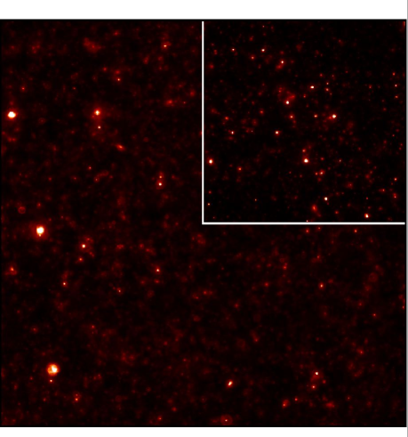
Figure 3.— Map of the thermal SZ effect in our AGN feedback and comparison runs (large panel and inset panel, respectively). Here the area of the largest panel is $(1.1{\rm deg})^{2}$ and the color scale runs from $\frac{\Delta T}{T}=0$ (black) to $-5\times 10^{-5}$ (white), (or 0 to -135 $\mu$K).

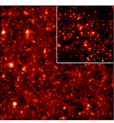
Figure 4.— Map of the logarithm of the thermal SZ effect, ranging from $\log(-\Delta T/T)=\log(1\times 10^{-6})$ (black) to $\log(-\Delta T/T)=\log(5\times 10^{-5})$ (white), with panels as in Figure 3. While the AGN simulation has a higher average Compton distortion, structure has been smoothed out on the smallest scales.

In Figure 3 we directly compare maps of the thermal SZ distortions from both these runs, integrated down to our final simulation redshift of $z=1.2.$ The maps clearly indicate a lack of small hot regions in the AGN feedback run relative to the comparison run. To help bring out the structure in these maps, we also plot the same data on a logarithmic scale in Figure 4. Here we see that the AGN feedback run has a higher average level of distortions, consistent with the $\left<y\right>$ evolution in Figure 2. Furthermore, while it is difficult to tell the overall level of the variance between the maps, it is clear that the scale of the structures is quite different. In particular, while the AGN feedback simulation has fewer small pockets of hot gas, these are compensated for by a number of larger and more diffuse heated regions.

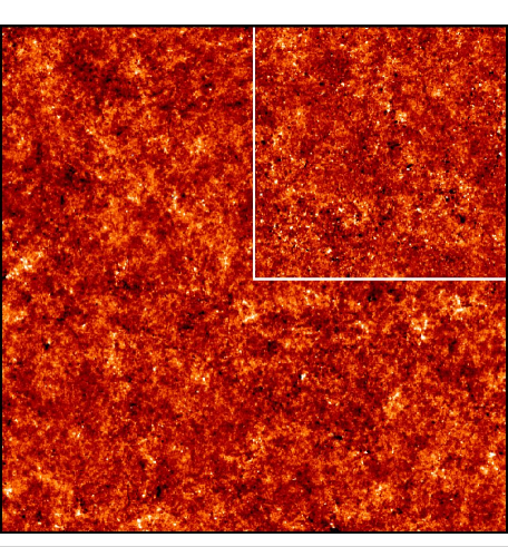
Figure 5.— Map of the kinetic SZ effect ranging from $\frac{\Delta T}{T}=-1\times 10^{-5}$ (black, moving away from the observer) to $1\times 10^{-5}$ (white, moving towards the observer), that is -27.3 to 27.3 $\mu$K.

Finally, the kinetic SZ maps, as shown in Figure 5, look similar in the two simulations. The differences in this case appear to be quite subtle, and must be distinguished by a more detailed, quantitative approach.

3.2. Power Spectrum

3.2.1 Results from Simulated Maps

The most common measure of CMB fluctuations is the angular power spectrum, obtained by decomposing the temperature distribution on the sky into spherical harmonics, $\Delta T/T({\bf\hat{n}})=\sum_{\ell,m}a_{\ell,m}Y_{\ell,m}({\bf\hat{n}}),$ and carrying out an average over the coefficients, $C_{\ell}=(2\ell+1)^{-1}\sum_{m=-\ell}^{\ell}a_{\ell,m}a^{*}_{\ell,m}.$ For a small field of view, as is the case for our constructed map, this is equivalent to performing a Fourier Transform to obtain

$${\tilde{\frac{\Delta T}{T}}}({\vec{\kappa}})=\int d^{2}{\vec{\theta}}\exp\left(-i{\vec{\kappa}}\cdot{\vec{\theta}}\right){\frac{\Delta T}{T}}({\vec{\theta}}),$$ (10)

(where $\vec{\theta}$ and $\vec{\kappa}$ are two dimensional vectors in the plane of the sky) and then carrying out an azimuthal average to obtain

$$C_{\ell}=P_{\rm ang}(\kappa=\ell)=\frac{1}{2\pi}\int d\phi{\tilde{\frac{\Delta T}{T}}}(\kappa,\phi){\tilde{\frac{\Delta T^{*}}{T}}}(\kappa,\phi),$$ (11)

where ${\vec{\kappa}}=(\kappa\cos\phi,\kappa\sin\phi).$ Finally, as an additional check one can use the fact that the mean squared temperature variance is equal to $\sum_{\ell}(2\ell+1)C_{\ell}/(4\pi).$

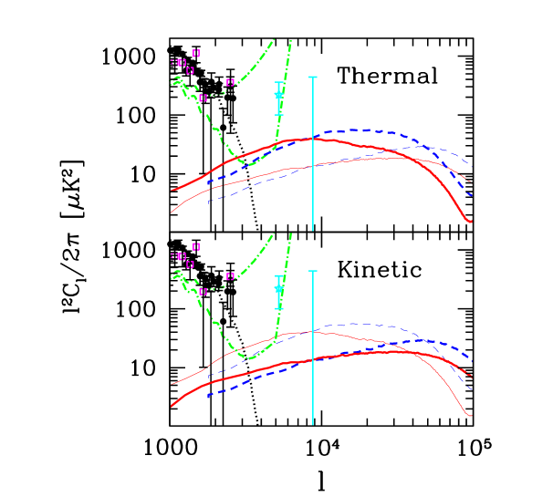
Figure 6.— Top: Power spectrum of the thermal SZ distortions in the AGN feedback run (thick solid line) and comparison run (thick dashed line), integrated down to $z=1.2$. The open squares are measurements by the CBI experiment (Bond et al. 2005),the solid points are measurements by the ACBAR experiment (Kuo et al. 2007), and the stars are measurements from the BIMA CMB Anisotropy Survey (Dawson et al. 2006). These are plotted around the primary anisotropy signal (dotted lines). For comparison, the thin solid and dashed lines show the kinetic SZ anisotropies for the AGN feedback and comparison run, as in the bottom panel. The dot-dashed lines show the level of anisotropies detectable by an experiment spanning a (20 deg)² area with a $\theta_{\rm FWHM}=2$ arcmin beam, with a noise level of (10 $\mu$K)² per arcmin² (upper line) and with a $\theta_{\rm FWHM}=1$ arcmin with a noise level of (2 $\mu$K)² per arcmin² (lower line). Bottom: Power spectrum from the kinetic SZ distortions in the AGN feedback run (thick solid line) and comparison run (thick dashed line), integrated down to $z=1.2$. Points and dot-dashed lines are as in the upper panel, and the thin lines are the thermal SZ distortions, shown for comparison.

In Figure 6 we plot the angular power spectrum from our AGN feedback and comparison simulations, averaging over 16 realizations of the maps: (4.4 deg)² in the AGN feedback case and (2.2 deg)² in the comparison case. As expected from a visual inspection of Figures 3 and 4 , AGN feedback has a clear impact on the thermal SZ signal, smoothing the structures at the smallest scales ($\ell\geq 10^{4}$) while at the same time adding large heated regions that increase the overall fluctuations at larger scales ($\ell\leq 10^{3}$). On the other hand, AGN feedback has only a weak impact on the kinetic SZ effect, slightly smoothing the smallest structures, without having a noticeable impact on larger scales. To some extent, the lack of this large-scale signal may be due to our choice of initially spherical outflows, which should not significantly add to the total integrated column of material moving towards or away from the observer along any line of sight. If outflows were extremely asymmetric, however, from eqs. (6) and (7) the ratio of the distortions in the kinetic to the thermal SZ effects would go as

$$\frac{b}{y}\approx\frac{v/c}{{kT}/{m_{e}c^{2}}}\approx\frac{m_{e}}{m_{p}(v/c)}.$$ (12)

For a typical outflow velocity of $v\approx 1000$ km/s, this gives $b/y\approx 1/6$, such that the even in this extreme case, the increase in $C_{\ell}$s due to the kinetic effect would be at least $\approx 30$ times smaller than the thermal signal.

However, even in the thermal case, the increase in the large-scale angular power spectrum is not dramatic. For comparison, in Figure 6 we have also plotted the primary CMB signal, as well as a summary of recent measurements from the CBI and ACBAR experiments. From these points it is clear that the secondary anisotropies seen in current experiments are not likely to have been imprinted by SZ distortions at $z\geq 1.2$, nor does the possible excess of small-scale power seen in the CBI experiment (see however, Kuo et al. 2007) appear to be related to AGN feedback.

3.2.2 Required Sensitivity and Resolution to detect AGN distortions

Pushing to the near future, however, the increase in the angular power spectrum due to AGN feedback is well within the range of upcoming experiments. To calculate these sensitivities we make use the simple estimate from Jungman et al. (1996), which gives the RMS noise at multipole $\ell$ as

$$\sigma_{\ell}=\left[\frac{2}{(2\ell+1)f_{\rm sky}}\right]^{-1/2}\left[C_{\ell}+(wf_{\rm sky})^{-1}e^{\ell^{2}\sigma_{b}^{2}}\right],$$ (13)

where $w\equiv(\sigma_{\rm pix}\theta_{\rm FWHM})^{-2}$ is the weight per solid angle, a pixel-size independent measure of the noise that is calculated from the full-width at half-max of the Gaussian beam, $\theta_{\rm FWHM},$ and the noise variance per $\theta_{\rm FWHM}\times\theta_{\rm FMWH}$ pixel, $\sigma_{\rm pix}^{2}.$ Finally, $\sigma_{b}=7.42\times 10^{-3}\times\theta_{\rm FHWM}$ is a measure of the beam size and $f_{\rm sky}$ is the fraction of the sky covered.

Comparing these measurements with the $C_{\ell}$s from our simulations, we see that the excess due to AGN feedback is easily measurable by an experiment with a typical full-width at half max beam size of $\theta_{\rm FWHM}\approx 1$ arcmin and a noise level of about (2 $\mu$K)² per arcmin${}^{2},$ scanning over a (20 deg)² patch of the sky. However, the most convincing constraints on AGN feedback are not likely to come from statistical constraints derived purely from the microwave background.

3.3. Cross Correlations

Unlike the primary microwave background signal, the SZ distributions are not well described by a Gaussian random field. Rather they contain a wealth of information beyond the angular power spectrum. In fact, as is particularly clear from Figures 3 and 4, the thermal SZ distribution is much more reminiscent of lower-redshift galaxy surveys than $z\approx 1000$ measurements. Furthermore, the structures seen in these maps are imprinted by galaxy activity, meaning that they are strongly correlated with the positions of sources in large-field optical and infrared surveys. With this in mind, we considered the cross-correlation of our maps with three types of optical sources:

• quasars, identified as newly-formed black holes that shine for $t_{d}=0.055r_{v}/v_{c}$ of the dynamical time of the system (as in §2.1)

• post-starburst elliptical (E+A) galaxies, identified as mergers observed within 200 Myrs of coalescence

• elliptical galaxies, identified as mergers observed at any time after coalescence.

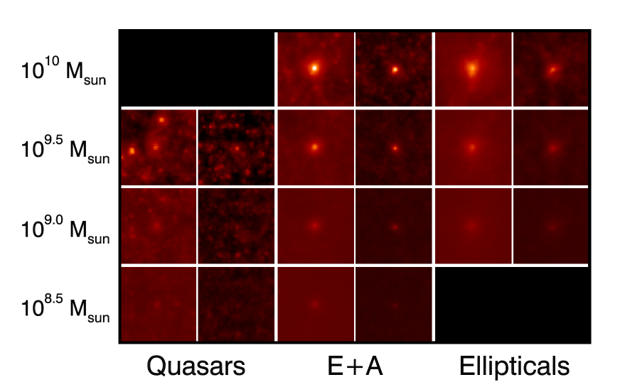
Figure 7.— Postage stamp images of the thermal SZ effect in a $6\times 6$ arcmin² region around various objects. Each pair of panels shows the distortions in the AGN run (left) and comparison run (right) averaged over all the sources in a (2.2 deg)² region of the sky. From top to bottom, the rows are labeled by the black hole masses, which range from $10^{10}{M_{\odot}}$ to $3\times 10^{8}{M_{\odot}}$. From left to right each of the pairs correspond to quasars, post-starburst ellipticals, and all elliptical galaxies. All panels are shown using a log scale from $\log(-\Delta T/T)=\log(2\times 10^{-5})$ (white) to $\log(-\Delta T/T)=\log(2\times 10^{-6})$ (black).

In Figure 7 we show the results of coadding the thermal SZ distortions around each of these objects as selected in a (2.2 deg)² region, made up of 4 maps in the AGN feedback run and 16 maps in the comparison run. The most obvious feature in this plot is the overall higher level of the SZ background in the AGN feedback run, a feature that is difficult to observe directly, as discussed in §2.1. Beyond this overall offset however, these images also uncover a substantial “halo” of SZ distortions, which is much higher in amplitude and more spatially extended in the AGN feedback case. While this excess is somewhat lost in the noise for quasars, which are the rarest sources, it is clearly and dramatically present in the coadded maps of the much more numerous E+A and elliptical galaxies. As expected from our discussion above, constructing similar coadded images of the kSZ effect yielded differences that were at least an order of magnitude smaller.

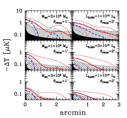
Figure 8.— Average excess thermal SZ distortions around quasars in our simulations. In each panel the thick solid line shows $\Delta T$ in the AGN feedback run, averaged over a (2.2 deg)² area of the sky. As a measure of the variance over the sky, the thin solid line shows the maximum and minimum $\Delta T$ signal in single (1.1 deg)² quadrants of this (2.2 deg)² map. Similarly, the thick dashed line shows the average $\Delta T$ in (2.2 deg)² of sky from the comparison run, bracketed by the maximum and minimum signals in quadrants. Finally, the shaded region shows the noise level attainable by averaging over all sources in (20 deg)², for an experiment with a noise-per-pixel of (10 $\mu$K)² per arcmin² (cross-hatched regions) and (2 $\mu$K)² per arcmin² (solid regions). The left panels show distortions as observed with a $\theta_{\rm FWHM}=1^{\prime}$ beam and the right panels show the same distortions for a $\theta_{\rm FWHM}=2^{\prime}$ beam. From top to bottom the panels correspond to black hole masses of $3\times 10^{9}{M_{\odot}}$, $1\times 10^{9}{M_{\odot}}$, and $3\times 10^{8}{M_{\odot}},$ respectively, as marked on the left panels, and the equivalent B-band luminosity is given in the right panels.

To further study the detectability of the much more promising thermal signal we processed each of the images in Figure 7 in a manner similar to how one might work with real data sets in the near future. First, we shifted each of them by the overall average $y$ distortion to account for the difficult to observe offset between the AGN feedback and comparison cases. Next, to approximate the angular resolution of the next generation of CMB telescopes, we convolved each image with Gaussian beams with $\theta_{\rm FWHM}$ of 1 and 2 arcmins. Finally, as coadding sources washes out any rotational asymmetries, we performed an azimuthal average to reduce noise while retaining the same information.

The results of this procedure are shown in Figure 8, for quasars with B-band luminosities above $1\times 10^{13}L_{\odot}$, $3\times 10^{12}L_{\odot},$ and $1\times 10^{12}L_{\odot}$, which correspond to black hole masses of $3\times 10^{9}{M_{\odot}}$, $1\times 10^{9}{M_{\odot}}$, and $3\times 10^{8}{M_{\odot}}.$ Each panel in this plot shows not only the average signal over all sources in a (2.2 deg)² region of the sky, but the maximum and minimum signal in any of the four ($1.1$ deg)² quadrants in this region, to give an impression of the variation in this quantity across the sky. While signals can vary substantially between quadrants, in all cases the overall average SZ signal is significantly higher in the AGN feedback case. As an estimate of the sensitivity of future experiments we also include on this plot a background noise level calculated as

$$\sigma_{\rm source}(\theta)=\left[\frac{\sigma^{2}_{\rm pix}}{N_{\rm sources}(2\pi\theta d\theta)}\right]^{1/2},$$ (14)

where $d\theta$ is the 1.1 deg/1024 = 0.0644 arcmin pixel size of our maps, $N_{\rm sources}$ is the number of sources that would be found in a (20 deg)² region of sky, and the pixel noise level, $\sigma_{\rm pix},$ is again estimated as (10 $\mu$K)² per arcmin² (cross-hatched region) and (2 $\mu$K)² per arcmin² (solid region).

The impact of AGN outflows is well above the noise for all sources, even if $\theta_{\rm FWHM}=2^{\prime}$ and $\sigma_{\rm pix}^{2}$ = (10 $\mu$K)² per arcmin². However, in most cases, the profile of the SZ signal above the noise is indistinguishable from a point source (which would appear on this plot as an inverted parabola that drops by a factor of two at a distance of $\theta_{\rm FWHM}/2$). At the same time quasars themselves are often significant microwave point sources. To estimate this intrinsic contribution we convert the flux per unit frequency, $F_{\nu}$, to CMB temperature units as

$$\Delta T = \left(\frac{dB_{\nu}}{dT}\right)^{-1}\ \frac{F_{\nu}}{\theta_{\rm FWHM}^{2}}$$ (15)

$$= \frac{1\mu{\rm K}}{0.0084\,{\rm mJy}}\left(\frac{1\,{\rm arcmin}}{\theta_{\rm FWHM}}\right)^{2}F_{\nu}\frac{(e^{x}-1)^{2}}{x^{4}e^{x}},$$

where $B_{\nu}$ is the Planck Function and, as in eq. (5), $x\equiv h\nu/kT_{\rm CMB}$ (Scott & White 1999). The ratio of $\nu L_{\nu}$ at microwave wavelengths to the quasars bolometric luminosity is $\sim 1/1000$ for “radio loud” objects which make up about $10\%$ of the population, and several orders of magnitude less for radio-quiet objects (Elvis et al. 1994). Estimating a typical luminosity distance to a quasar as $\approx$ 3000 Mpc $h^{-1}$ and considering a typical observing frequency of 100 GHz this gives

$$\Delta T\approx\frac{M_{\rm BH}}{10^{6}{M_{\odot}}}\left(\frac{1\,{\rm arcmin}}{\theta_{\rm FWHM}}\right)^{2}\mu{\rm K},$$ (16)

which is much larger than the thermal SZ signal.

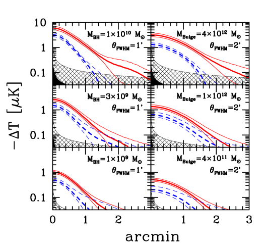
Figure 9.— Average excess thermal SZ distortions around post-starburst galaxies in our simulations, observed within 200 Mys of a merger. As there are many more of these objects than quasars, we select slightly larger objects in this figure than in Figure 8. Thus from top to bottom the panels correspond to black hole masses of $1\times 10^{10}{M_{\odot}}$, $3\times 10^{9}{M_{\odot}}$, and $1\times 10^{9}{M_{\odot}}$ (marked on the left panels), or equivalent bulge masses of $4\times 10^{12}{M_{\odot}}$, $1\times 10^{12}{M_{\odot}},$ and $4\times 10^{11}{M_{\odot}}$ (marked on the right panels). Otherwise the panels, lines, and shaded regions are defined as in Figure 8. Thus, the left panels show distortions as observed with a $\theta_{\rm FWHM}=1^{\prime}$ beam and the right panels show the same distortions for a $\theta_{\rm FWHM}=2^{\prime}$ beam; The thick solid (AGN feedback) and dashed (comparison) lines show the average value of the SZ distortions averaged over all sources in a (2.2 deg)² region of the sky, bracketed by the maximum and minimum signal in (1.1 deg)² quadrants; and the shaded regions show the noise levels attainable by averaging over (20 deg)${}^{2},$ with instrument noise as in Figure 8.

While this can be reduced substantially by selecting radio-quiet quasars, a better approach is to work with objects observed at later times after the merger. In Figure 9 we show the azimuthally averaged excess thermal SZ contribution around post-starburst galaxies, identified as mergers observed after the quasar phase, but within 200 Myrs after coalescence. Here we have converted each black hole mass to its corresponding stellar bulge mass using a factor of $\approx 400$ as obtained from the analysis in Marconi & Hunt (2003). Working with these sources has two main advantages. Firstly, as they are much more common, one can consider slightly larger bulges and hence larger and more spatially extended SZ distortions, while at the same time improving the number of sources that can be coadded in a fixed region of the sky. Furthermore, as the nuclear luminosities are typically more than 100 times less during this phase (e.g. Hopkins et al. 2007), point source subtraction is much easier, although some exclusion of radio-loud sources may still be necessary.

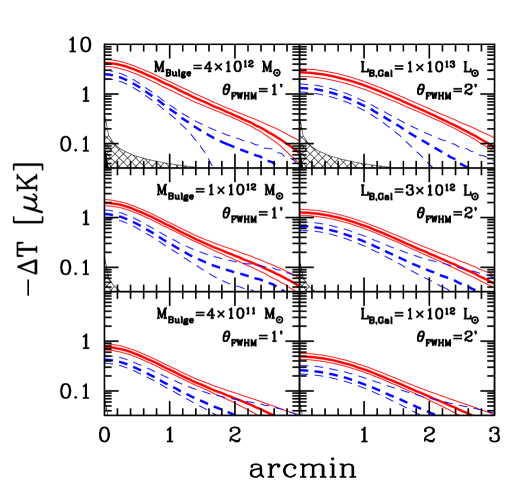
Figure 10.— Average excess thermal SZ distortions around all bulges in our simulations. Mass limits, beam sizes, and symbols are as in Figure 9. Right panels are labeled with estimated total bulge $L_{B}$ luminosities following Marconi & Hunt (2003)
.

In Figure 10 we show the SZ contribution obtained by coadding all bulges observed at any time after the initial quasar phase. Again we have converted black hole mass into bulge mass as well as into overall B-band luminosity following observed relations (Marconi & Hunt 2003). Extending our analysis in this way has only a weak impact on the SZ profile, while at the same time improving the statistics even further. In this case the complete spatial profiles of the sources are observable with more than 10 $\sigma$ precision out to very large radii, clearly tracing out the impact of AGN feedback. Note that these sources are relatively easy to detect, as even given a typical luminosity distance of $10^{4}$ Mpc, they are readily observed by a photometric survey with an overall magnitude limit of $m_{B}\approx 22.$

Furthermore, the level of thermal $y$ distortions observed by coadding around bulges is a precise and linear measure of the most important quantity for modeling the impact of AGN outflows on galaxy formation. Integrating eq. (6) over a patch of sky around a source we have

$$\int d{\vec{\theta}}y({\vec{\theta}})=\frac{\sigma_{T}}{m_{e}c^{2}}\frac{1}{l_{\rm ang}^{2}}\int dVn_{e}(V)k[T_{e}(V)-T_{\rm CMB}],$$ (17)

where $l_{\rm ang}$ is the angular diameter distance to the source, ${\vec{\theta}}$ is a vector in the plane of the sky in units of radians, and the volume integral is performed over the heated region around the source. But this integral is simply $(2/3)E_{\rm thermal}(1+A)/(2+A)$ where $A=0.08$ is the cosmological number abundance of helium. The line-of-sight integral of the pressure has thus been transformed into a volume integral of the pressure. This means that by integrating the Compton distortions over the sky we can directly measure the thermal energy added to the IGM for each object. Rewriting eq. (17) in terms of angles in arcminutes and the low-frequency microwave background distortions in units of $\mu K$ this becomes

$$E_{\rm thermal}=-4.8\times 10^{60}\,{\rm ergs}\,\,\,\,\tilde{l}_{\rm ang}^{2}\frac{\int d{\vec{\theta}}\Delta T({\vec{\theta}})}{\mu K\,{\rm arcmin}^{2}},$$ (18)

where $\tilde{l}_{\rm ang}$ is the angular distance in units of $3000$ Mpc and $E_{\rm thermal}$ is the total excess thermal energy associated with the source, that is the thermal energy gained from the initial collapse of the baryons, plus the contribution from the AGN, minus losses due to cooling and $PdV$ work done during expansion.

3.4. Measuring AGN Feedback

Putting these results together, a clear and direct way to constrain AGN feedback presents itself. This can be summarized as follows:

• Obtain SZ data with 1 or 2 arcminute resolution at a noise level of a few $\mu K$ per arcmin² in a $\approx 400$ deg² patch of the sky in which near infrared or optical photometry is available to a moderately deep magnitude limit (such as $m_{B}\approx 22$).

• Select all quiescent early-type galaxies with photometric redshifts in the essential $z=1-3$ redshift range for AGN feedback. Alternatively, if sufficiently good photometry is available, one can also study the subset of post-starburst (E+A) galaxies.

• If possible, use radio observations to reject point sources that may contaminate the thermal SZ signal.

• Compute the excess thermal SZ signal summed within a $\approx$ 2 arcminute radius around each source, and use this to compute the total thermal energy as per eq.  (18).

• Bin the results as a function stellar mass, and average over each bin to compute the total average IGM thermal energy input associated with bulges as function of their stellar mass.

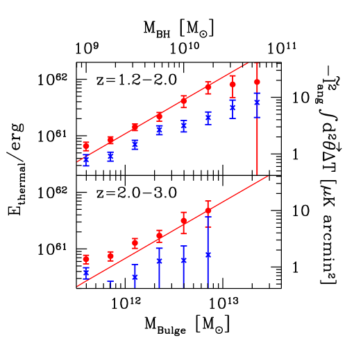
Figure 11.— IGM thermal energy computed from eq. (18) as a function of bulge stellar mass in our AGN feedback (solid points) and comparison (crosses) simulations. In each bin the point shows the results of averaging over all sources in a $\log_{10}(M_{\rm bulge})=0.25$ bin surrounded by error bars that account for both the intrinsic variation between sources and the fact that multiple maps have been derived from the same simulation (see text). The solid lines, on the other hand, show the energy input added around bulges in our AGN feedback simulation, as per eq.  (4). In the upper panel we consider all bulges in the redshift range from $z=1.2-2.0,$ and in the lower panel from $z=2.0-3.0.$

The results of carrying out this procedure over (2.2 deg)² of sky calculated from our simulations are shown in Figure 11. Here we have grouped all bulges in logarithmic bins of stellar mass with width $0.25$, again taking a fixed ratio of 400 between $M_{\rm bulge}$ and $M_{\rm BH}.$ To calculate the uncertainty in each bin we have accounted both for Poisson noise and intrinsic scatter, taking $\sigma_{\rm bin}(E_{\rm thermal})=[\bar{E}_{\rm thermal,bin}+\sigma_{\rm source}(E_{\rm thermal})]/\sqrt{N_{\rm bin}},$ where $\bar{E}_{\rm thermal,bin}$ is the average thermal energy in a given bin, $\sigma_{\rm source}(E_{\rm thermal})$ is the RMS scatter between sources in a given bin, where we computed $N_{\rm bin}$ conservatively as the number of sources in a given bin relative to a signal realization of the map (1/4 of the [2.2 deg]² region in the AGN feedback run and 1/16 of this region in the comparison run).

At both high and low redshifts the AGN feedback run shows a clear excess, which scales linearly with $M_{\rm bulge}$ as expected from eq. (4). For comparison, we use this equation to plot the energy added to the IGM as a function of bulge mass. Since kinetic energy is converted into thermal energy as the outflows accrete material, and as radiative losses are small for these objects (e.g. Oh & Benson 2003; Scannapieco & Oh 2004), we expect that most of this energy should be observable as $E_{\rm thermal}.$ In fact, this figure shows that at both low and high redshift, the thermal SZ excess closely traces this energy input as a function of bulge mass. Thus AGN feedback is not only detectable by the SZ effect, but the level of this feedback as a function of mass can be obtained directly from SZ measurements.

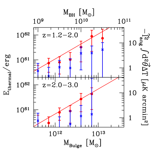
Figure 12.— Thermal energy around post-starburst galaxies as a function of bulge stellar mass. Panels and symbols are as in Figure 11.

Finally, in Figure 12, we plot $E_{\rm thermal}$ for the post-starburst galaxies in our simulations. As there are fewer of these objects, this results in a higher overall scatter than in the case of all bulges, but the results are otherwise similar and consistent with the level of excess energy added to the AGN feedback run. While this is to be expected given the instantaneous and impulsive nature of the outflows in our simulation, comparisons of post-starburst with other bulges may nevertheless help to distinguish this type of feedback from more gradual AGN heating, as suggested, for example, in Croton et al. (2006).

4. Conclusions

Microwave background measurements have played a key role throughout cosmology: establishing the modern inflationary model, constraining the initial conditions for structure formation, and providing precise measurements of cosmological parameters. Yet at smaller scales, the potential of CMB measurements is largely untapped.

At the same time, detailed observations at lower redshifts have uncovered the central importance of nongravitational heating, which is likely to be associated with outflows from AGN. Although the details of this process remain uncertain, we have shown using a suite of large numerical simulations that the key observations constraining this process may once again come from the microwave background. While AGN outflows impact the CMB both through their peculiar motions and through IGM heating, it is the thermal SZ signal that provides the most detailed measurements. Working purely with CMB observations, AGN feedback can be constrained both through a difficult to measure overall offset in the frequency spectrum, and a more easily detected shift in CMB anisotropies from $\approx 1/10$ arcmin to $\approx 1$ arcmin scales.

Although changes in the angular power spectrum from this shift are marginally detectable with the upcoming generation of small-scale microwave telescopes, the true test of AGN feedback will come from the cross-correlation of this data with infrared and optical surveys. In particular, coadding the CMB signal around quasars, post starburst, and quiescent elliptical galaxies from our simulations shows a systematic “halo” of SZ distortions around each of these objects, which is much higher in amplitude and more spatially extended in the AGN feedback case. Also, while contamination from point source emission make quasars difficult to work with, the excess signal is clearly detectable for both E+A and older elliptical galaxies, which can be selected with only moderately deep $m_{B}\approx 22$ photometry.

Furthermore, as the thermal SZ effect is proportional to the line of sight integral of the pressure, summing up the excess distortion in a patch of sky around each type of source provides a sensitive and direct measure of the thermal energy associated with feedback. In fact, carrying out this procedure on our simulation we have shown that we can easily recover not only the overall level of AGN feedback, but its dependence on galaxy mass, redshift, and galaxy type. Although it provides a popular and elegant solution to many outstanding problems, the impact of IGM heating by AGN outflows remains perhaps the most uncertain outstanding issue in galaxy formation. Working together with large-field optical surveys, small-scale CMB experiments will soon be able to place strong constraints on this missing piece in our physical understanding of the history of our universe.

References

- (1)
- (2) Agertz, O. et al. 2006, MNRAS, submitted, (astro-ph0610051)
- (3) Arnaud, M. & Evrard, E. 1999, MNRAS, 305, 613
- (4) Arnouts, S. et al. 2005, ApJ, 619, L43
- (5) Babul, A., Balogh, M. L., Lewis, G. F., & Poole, G.B. 2002, MNRAS, 330, 329
- (6) Barger, A. J., Cowie, L. L., Mushotzky, R. F., Yang, Y., Wang, W.-H., Steffen, A. T., & Capak, P. 2005, AJ, 129, 578
- (7) Barkana, R., & Loeb, A. 1999, ApJ, 523, 54
- (8) Battye, R. A., & Weller. J. 2003 Phys Rev. D., 68, 3506
- (9) Bell, E. F. et al. 2006, ApJ, 640, 241
- (10) Birnboim, Y., Dekel, A., & Neistein, E. 2007, MNRAS, submitted (astro-ph/0703435)
- (11) Bond, J. R. et al. 2005, ApJ, 626, 12
- (12) Brüggen, M., Ruszkowski, M., Hallman, E. 2005, ApJ, 630,740
- (13) Cattaneo, A., Dekel, A., Devriendt, J., Guiderdoni, B., & Blaziot, J. 2006, MNRAS, 370, 165
- (14) Cavaliere, A., Menci, N., & Tozzi, P. 1998, ApJ, 501, 493
- (15) Chartas, G., Brandt. W. N., Gallagher, S.C., & Proga, D. 2007, AJ, 113, 1849
- (16) Chatterjee, S. & Kosowsky, A. 2007, ApJL, 661, 113
- (17) Couchman, H. M. P. 1991, ApJ, 386, L23
- (18) Cowie, L. L., Songaila, A., Hu, E. M., & Cohen, J. G. 1996, AJ, 112, 839
- (19) Croton, D. et al. 2006, MNRAS, 365, 11
- (20) da Silva A. C., Barbosa, D., Liddle, A. R., & Thomas, P. A. 2000, MNRAS, 317, 37
- (21) Dawson, K. S., Holzapfel, W. L., Carlstrom, J. E., Joy, M., & LaRoque, S. J. 2006, ApJ, 647, 13
- (22) de Kool, M., et al. 2001, ApJ, 548, 609
- (23) Dekel, A., & Birnboim, Y. 2006, MNRAS, 368, 2
- (24) Di Matteo, T., Springel, V., & Hernquist, L. 2005, Nature, 433, 604
- (25) Di Matteo, T., Colberg, J., Springel, V., Hernquist, L., & Sijacki, D. 2007, ApJ, submitted (arXiv:0705.2269v1)
- (26) Dobbs, M. et al. 2006, New Astronomy Reviews, 50, 960
- (27) Eisenstein, D. & Hu, W. 1999, ApJ, 511, 5
- (28) Elvis, M. et al. 1994, ApJS, 94,1
- (29) Ferrarese, L. 2002, ApJ, 578, 90
- (30) Furlanetto, S., & Loeb, A. 2001, ApJ, 556, 619
- (31) Gingold, R. A. & Monaghan, J. J. 1977, MNRAS, 181, 375
- (32) Granato, G. L., De Zotti, G., Silva, L., Bressan, A., & Danese, L. 2004, ApJ, 600, 580
- (33) Hanany, S. et al. 2000, ApJ, 545, 5
- (34) Helsdon, S.F., & Ponman, T.J. 2000, MNRAS, 315, 256
- (35) Hobson, M. P. & Magueijo, J. 1996, MNRAS 283, 1133
- (36) Hopkins, P.F., Hernquist, L., Cox, T. J., & Kereš, D. 2007, ApJ, submitted (arXiv:0706.1243)
- (37) Holder, G. P., Mohr, J. J., Carlstrom, J. E., & Evrard, A. E., Leitch, E. 2000, ApJ, 544, 629
- (38) Jungman, G., Kamionkowski, M., Kosowsky, A., & Spergel, D. N. 1996, Phys. Rev. Lett. 76, 1007
- (39) Kereš, D., Katz, N., Weinberg, D. H., & Davé 2005, MNRAS, 363, 2
- (40) Khochfar, S., & Ostriker, J. P. 2007, ApJ, submitted, (arXiv:0704.2418)
- (41) Kosowsky, A. et al. 2006, New Astron. Rev. 50, 969
- (42) Kravtsov, A. V., & Yepes, G. 2000, MNRAS, 318, 227
- (43) Kuo et al. 2007, ApJ, 664, 678
- (44) Loh, M., et al. 2005, AAS Meeting Abstracts, 207, 4101
- (45) Lucy, L. B. 1977, AJ, 82, 1013
- (46) Majumdar, S., Nath, B., & Chiba, M. 2001, MNRAS, 324, 537
- (47) Majumdar, S., & Mohr, J. J. 2003, ApJ, 585, 603
- (48) Marconi, A., & Hunt, L. 2003, ApJL, 589, 21
- (49) Mason, B. S. et al. 2003, ApJ, 591, 540
- (50) Mauskopf, P. D. et al. 2000, ApJ, 536, 59
- (51) Merritt, D., & Ferrarese, L. 2001, ApJ, 547, 140
- (52) Nath, B. B., & Roychowdhury, S. 2002, MNRAS, 333, 145
- (53) Oh, S. P., Cooray, A., & Kamionkowski, M. 2003, MNRAS, 342, 20
- (54) Oh, S. P., & Benson, A. J. 2003, MNRAS, 342, 664
- (55) Pei, Y. C. 1995, ApJ, 438, 623
- (56) Perlmutter, S., et al. 1999, ApJ, 517, 565
- (57) Rees, M., J., & Ostriker, J. P. 1977, MNRAS, 179, 541
- (58) Refregier, A., Komatsu, E., Spergel, D. N., & Pen, U.-L. 2000, Phys. ‘Rev. D, 61, 123001
- (59) Riess et al. 1998, AJ, 116, 1009
- (60) Roncarelli, M., Moscardini, L., Borgani, S., & Dolag, K. 2007, MNRAS, submitted (astro-ph/0701680)
- (61) Ruhl, J. E. et al. 2004, Proc. SPIE, 5498, 11
- (62) Scannapieco, E., Thacker, R. J., & Davis, M. 2001, ApJ, 557, 605
- (63) Scannapieco, E. & Oh, S. P. 2004, ApJ, 608, 62
- (64) Scannapieco, E., Silk, J., & Bouwens, R. 2005, ApJ, 635, L13
- (65) Scaramella, R., Cen, R., & Ostriker, J. P. 1993, ApJ, 416, 399
- (66) Schulz, A. E., & White, M. 2003, ApJ, 586, 72
- (67) Scott, D., & White, M. 1999, A&A, 346, 1
- (68) Seljak, U., Burwell, J., & Pen, U.-L. 2001, Phys. Rev. D., 63, 063001
- (69) Silk, J. 1977, ApJ, 211, 638
- (70) Smoot, G. F. et al. 1992, ApJ, 396, 1
- (71) Spergel, D. et al. 2003, ApJS, 148, 175
- (72) Spergel, D. et al. 2007, ApJS, 170, 377
- (73) Springel, V., White, M., & Hernquist, L. 2001, ApJ, 549, 681
- (74) Sunyaev, R. A., & Zel’dovich, Ya. B. 1970, Ap&SS, 7, 3
- (75) Sunyaev, R. A., & Zel’dovich, Ya. B. 1972, Comments Astrophys. Space Phys., 4, 173
- (76) Thacker, R. J. & Couchman, H. M. P. 2006, Computer Physics Communications, 174, 540
- (77) Thacker, R. J., Scannapieco, E., & Couchman, H. M. P. 2006, ApJ, 653, 86 (TSC06)
- (78) Tremaine, S., et al. 2002, ApJ, 574, 740
- (79) Treu, T., Ellis, R. S., Liao, T. X., & van Dokkum, P. G. 2005, ApJ, 622, L5
- (80) Ueda, Y., Akiyama, M., Ohta, K., & Miyaji, T. 2003, ApJ, 598, 886
- (81) Vianna, P. T. P. & Liddle, A. 1996, MNRAS, 281, 323
- (82) White, M., Hernquist, L., & Springel, V. 2002, ApJ, 579, 16
- (83) Wu, K. K. S., Fabian, A. C., & Nulsen, P. E. J. 2000, MNRAS, 318, 889
- (84) Wyithe, J. S. B., & Loeb, A., 2002, ApJ, 581, 886
- (85) Zhang, P., Pen, U.-L., & Wang, B. 2000, ApJ, 557, 555
- (86)