Two physical characteristics of numerical apparent horizons

Abstract

This article translates some recent results on quasilocal horizons into the language of $(3+1)$ general relativity so as to make them more useful to numerical relativists. In particular quantities are described which characterize how quickly an apparent horizon is evolving and how close it is to either equilibrium or extremality.

1 Introduction

In $(3+1)$-dimensional numerical relativity an apparent horizon in a three-dimensional spacelike slice $\Sigma_{t}$ is the outermost smooth two-surface whose whose outward null expansion vanishes [1, 2]. Then an apparent horizon world-tube is a three-surface $H$ foliated by two-surfaces $S_{t}\subset\Sigma_{t}$ with vanishing outward null expansion. Such surfaces have been an active topic of research in mathematical relativity for the last 10-15 years (see [3, 4, 5] for reviews or the reference section of [6] for more recent papers) and results from that work are now beginning to be applied to numerical relativity [7, 8].

This short paper continues this tradition by translating results from recent papers into the language of $(3+1)$-dimensional relativity. We first consider the recent work on slowly evolving horizons [9, 10, 6]. These papers found conditions under which a horizon can be considered to be in a quasi-equilibrium state. Intuitively, slowly evolving horizons are ‘‘almost" isolated [11] and so ‘‘nearly" null. Here we shall focus on an expansion parameter that arose from that work. This parameter is necessarily small for slowly evolving horizons, but even if it isn’t small it can be used to invariantly characterize the rate of expansion of horizons. It is to this end that we discuss it here, with a particular eye to tracking how quickly a black hole settles down to equilibrium after a merger or formation.

Second we consider a parameter that characterizes how close an apparent horizon is to being extremal[12]. Extremality in this case is a generalization of the well-known bound on the maximum angular momentum of a Kerr black hole relative to its mass (or equivalently surface area). For apparent horizons this turns out to be related to the expansion parameter and places a bound on the maximum angular momentum relative to the intrinsic geometry of the horizon. The immediate use for this parameter would be to study the proximity to extremality of post-merger black holes.

2 Horizons in (3+1)-dimensional gravity

Let $(M,g_{ab},\nabla_{a})$ be a four-dimensional spacetime which is foliated by spacelike three-surfaces $\{(\Sigma_{t},h_{ij},D_{i})\,;t_{1}\leq t\leq t_{2}\}$ where $h_{ij}$ is the induced metric and $D_{i}$ is the compatible covariant derivative. Note the indices; throughout this paper we will use early-alphabet latin indices for four-dimensional quantities and mid-alphabet latin indices for those defined in the three-slices. We use $e$ to denote the pull-back/push-forward operator between the various spaces.

Next let $T^{a}$ be a compatible time-evolution vector field generating a flow which maps the $\Sigma_{t}$ into each other. That is ${\cal L}\,_{T}t=1$. In the usual way this may be broken up as

$$T^{a}=N\hat{u}^{a}+V^{a}\,,$$ (1)

where $N$ is the lapse function, $V^{a}=e^{a}_{i}V^{i}$ is the spacelike shift vector field for some $V^{i}\in T\Sigma_{t}$, and $\hat{u}^{a}$ is the future-pointing timelike normal vector field to the $\Sigma_{t}$.

Finally we choose our sign convention so that the extrinsic curvature $K_{ij}$ of the $\Sigma_{t}$ in $M$ is

$$K_{ij}=\frac{1}{N}(\dot{h}_{ij}-{\cal L}\,_{V}h_{ij})=e_{i}^{a}e_{j}^{b}\nabla_{a}\hat{u}_{b}\,,$$ (2)

where the dot indicates a Lie derivative with respect to $T^{a}$.

Now, let $S_{t}$ be a closed two-surface in a slice $\Sigma_{t}$ and write its outward-pointing unit normal as $\hat{s}^{i}$. Then future-outward and future-inward pointing null normals to $S_{t}$ in $M$ can be written as

$$\ell^{a}=f(\hat{u}^{a}+\hat{s}^{a})\;\;\mbox{and}\;\;n^{a}=\frac{1}{2f}\left(\hat{u}^{a}-\hat{s}^{a}\right)\,,$$ (3)

where $\hat{s}^{a}=e^{a}_{i}\hat{s}^{i}$ and $f$ is an arbitrary positive function: we have adapted the standard cross-normalization $\ell\cdot n=-1$ so there is the only free parameter in their definition. For $f=1$ we denote this pair of null normals as $(\ell^{a}_{o},n^{a}_{o})$ as shown in Fig. 1.

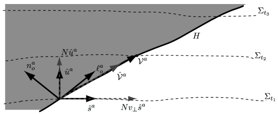
Figure 1: A two-dimensional cross-section of a spacetime $M$ foliated by spacelike three-surfaces $\Sigma_{t}$. $H$ is an apparent horizon world-tube which is foliated by the spacelike two-surfaces $S_{t}=H\cap\Sigma_{t}$.

We write the induced two-metric on $S_{t}$ as $\tilde{q}_{AB}$ (using capital Latin indices for such two-dimensional quantities) and note that

$$\tilde{q}^{ab}\equiv e^{a}_{A}e^{b}_{B}\tilde{q}^{AB}=g^{ab}+\ell^{a}n^{b}+\ell^{b}n^{a}\;\;\mbox{and}\;\;\tilde{q}^{ij}\equiv e^{i}_{A}e^{j}_{B}\tilde{q}^{AB}=h^{ij}-\hat{s}^{i}\hat{s}^{j}\,.$$ (4)

Then the outward and inward null expansions are, respectively,

$$\theta_{(\ell)}=\tilde{q}^{ab}\nabla_{a}\ell_{b}=f(\tilde{q}^{ij}K_{ij}+\tilde{q}^{ij}D_{i}\hat{s}_{j})\;\;\mbox{and}\;\;\theta_{(n)}=\tilde{q}^{ab}\nabla_{a}n_{b}=\frac{1}{2f}(\tilde{q}^{ij}K_{ij}-\tilde{q}^{ij}D_{i}\hat{s}_{j})\,.$$ (5)

As noted in the introduction, on a numerical apparent horizon $\theta_{(\ell)}=0$ and in practical simulations where there are known to be black holes in the initial data, this will usually be a sufficient condition to identify a black hole boundary. A key word in the previous sentence is ‘‘usually" and we will return to the potential complications in section 4.

For now, however, we will assume that an apparent horizon finding algorithm [2] has been used to identify $\theta_{(\ell)}=0$ surfaces on each $\Sigma_{t}$ over some range of $t$ and further that over that range their union is a smooth three-surface $H$. Then we can always find a horizon evolution vector field $\mathcal{V}^{a}$ that is normal to the $S_{t}$ and maps these surfaces into each other. Since the $S_{t}\subset\Sigma_{t}$ we can write

$$\mathcal{V}^{a}=N(\hat{u}^{a}+v_{\perp}\hat{s}^{a})\,,$$ (6)

where $N$ is again the lapse and $v_{\perp}$ is the the ‘‘velocity" of the horizon relative to the foliation. For a null horizon parallel to $\ell^{a}$, $v_{\perp}=1$ while for a spacelike and expanding horizon $v_{\perp}>1$.

3 Expansion

We now consider the first of the physical characteristics: the rate of expansion of the horizon. Relative to the foliation, the rate of change of the area element $\sqrt{\tilde{q}}$ is

$${\cal L}\,_{\mathcal{V}}\sqrt{\tilde{q}}=\sqrt{\tilde{q}}\left(\tilde{q}^{ab}\nabla_{a}\mathcal{V}_{b}\right)=\sqrt{\tilde{q}}\left(N(v_{\perp}-1)\tilde{q}^{ij}D_{i}\hat{s}_{j}\right)\,,$$

where we have made use of the fact that $\theta_{(\ell)}=0\Leftrightarrow\tilde{q}^{ij}K_{ij}=-\tilde{q}^{ij}D_{i}\hat{s}_{j}$ (which could also be used to rewrite the last line in terms of $\tilde{q}^{ij}K_{ij}$). This expansion is manifestly dependent on the lapse $N$ and so the coordinate $t$ labelling of the hypersurfaces $\Sigma_{t}$. However, if $H$ is not null there is an obvious remedy to this problem : calculate the rate of expansion with respect to the unit $\hat{\mathcal{V}}^{a}=\mathcal{V}^{a}/||\mathcal{V}||$ instead of $\mathcal{V}$ itself. Then the expansion relative to $\hat{\mathcal{V}}$ is

$$\theta_{(\hat{\mathcal{V}})}=\alpha\sqrt{\left|\frac{v_{\perp}-1}{v_{\perp}+1}\right|}\tilde{q}^{ij}D_{i}\hat{s}_{j}\,,$$ (7)

where $\alpha=\operatorname{sgn}(v_{\perp}-1)$. Note that $\theta_{(\hat{\mathcal{V}})}$ goes to zero as $v_{\perp}\rightarrow 1$ even though $\hat{\mathcal{V}}^{a}$ itself diverges.

To better understand $\theta_{(\hat{\mathcal{V}})}$, we return to four-dimensions and the formalism developed for slowly evolving horizons [9, 6]. There, $\mathcal{V}^{a}$ was written in terms of the null normals and a parameter $C$:

$$\mathcal{V}^{a}=\ell^{a}-Cn^{a}\,.$$ (8)

Then the foliation of the horizon fixes both a scaling of the null vectors and $C$. Comparing with (6) it is straightforward to see that in the $(3+1)$-formalism these take the form:

$$f=N(1+v_{\perp})/2\;\;\mbox{and}\;\;C={N^{2}}(v_{\perp}^{2}-1)/2\,.$$ (9)

The value of $C$ fixes the signature of the horizon: $C>0\Leftrightarrow|v_{\perp}|>1\Leftrightarrow$ $H$ is spacelike, $C=0\Leftrightarrow|v_{\perp}|=1\Leftrightarrow$ $H$ is null, and $C<0\Leftrightarrow|v_{\perp}|<1\Leftrightarrow$ $H$ is timelike. We can rewrite

$$\theta_{(\hat{\mathcal{V}})}=-\alpha\sqrt{|{C}/{2}|}\theta_{(n)}\,,$$ (10)

where $\alpha=\operatorname{sgn}(C)$. In this form $\theta_{(\hat{\mathcal{V}})}$ (or actually its square) is the most important of several quantities used to decide whether or not a horizon is ‘‘almost" isolated and so in quasi-equilibrium with its surroundings. Among other properties such horizons will obey approximate zeroth law and first laws of black hole mechanics with all fluxes being calculated relative to the $\ell^{a}$ normals (as if they where truly null). Some intuition for how dramatically a horizon can evolve and still be counted as in a quasi-equilibrium state can be gained from the examples of [10].

To be mathematically certain about such a classification one needs to track $\theta_{(\hat{\mathcal{V}})}^{2}$ and the other quantities point-by-point on the horizons. However to get a quick idea of the rate of expansion (and proximity to equilibrium) it is convenient to have a single, dimensionless, number to calculate. Such a quantity can be obtained by integrating the square of $\theta_{(\hat{\mathcal{V}})}$ over $S_{t}$:

$$\epsilon^{2}_{area}=\frac{1}{2}\int_{S_{t}}\mspace{-10.0mu}d^{2}x\sqrt{\tilde{q}}|C|\theta_{(n)}^{2}=\int_{S_{t}}\mspace{-10.0mu}d^{2}x\sqrt{\tilde{q}}\left|\frac{v_{\perp}-1}{v_{\perp}+1}\right|(\tilde{q}^{ij}D_{i}\hat{s}_{j})^{2}\,.$$ (11)

In spherical symmetry this is proportional to $(dR_{H}/ds)^{2}$, where $R_{H}=\sqrt{a/4\pi}$ is the areal radius of $S_{t}$ and $s$ is the arclength ‘‘up" the horizon along a flow line of $\mathcal{V}^{a}$.

4 Apparent horizons as black hole boundaries

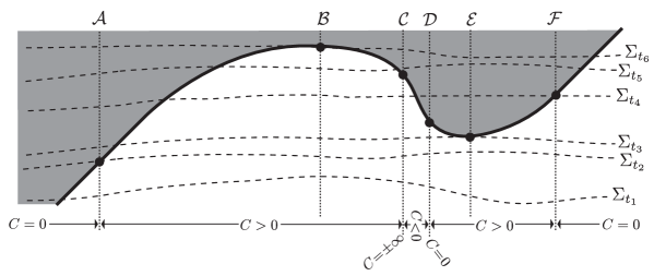
Figure 2: A horizon $H$ with $\theta_{(\ell)}=0$ and $\theta_{(n)}<0$ evolves between equilibrium states. Here, null horizons have slopes of $\pm 45^{\circ}$, spacelike horizons have slopes from $-45^{\circ}$ to $45^{\circ}$, and timelike membranes have the steeper slopes outside of that range. Thus before $\mathcal{A}$, $H$ is in equilibrium and null (parallel to $\ell^{a}$). From $\mathcal{A}\rightarrow\mathcal{C}$ it is expanding and spacelike. At $\mathcal{C}$ it is momentarily null (parallel to $n^{a}$) and $\epsilon_{area}$ diverges. From $\mathcal{C}\rightarrow\mathcal{D}$, $H$ is a timelike membrane before becoming null again at $\mathcal{D}$. Finally from $\mathcal{D}\rightarrow\mathcal{F}$ it is again a dynamical horizon before becoming isolated and quiescent after $\mathcal{F}$. Between $\mathcal{C}$ and $\mathcal{D}$, $H$ is super-extremal while at those points it is extremal.

We now return to the ‘‘usually" that followed equation (5) and consider when we can definitively associate a black hole with an apparent horizon. Following Penrose [14] we take the existence of fully trapped surfaces ($\theta_{(\ell)}<0$, $\theta_{(n)}<0$) as being the key characteristic of black holes. Together with the null energy condition (and some more technical assumptions) the existence of trapped surfaces both implies a spacetime singularity somewhere in their causal future and, if the spacetime is asymptotically flat, an enveloping event horizon [13]. Then, taking the set of all points that lie on trapped surfaces as the interior of a black hole, one would intuitively expect the boundary of that region to be foliated by two-surfaces $S_{t}$ with $\theta_{(\ell)}=0$ and $\theta_{(n)}<0$, and further expect that slight inwards deformations of the $S_{t}$ should turn them into fully trapped surfaces. These ideas are the foundation for both the mathematical relativity definition of an apparent horizon (the closure of the boundary of the set of all points lying on trapped surfaces in a given $\Sigma_{t}$) [13] as well as Hayward’s trapping horizons [15].

Though in reality things turn out to be more complicated (see for example the discussion of ‘‘wild" trapped surfaces in [16] or the counter examples in [17]) the motivation remains valuable and $\theta_{(\ell)}=0$ ‘‘boundaries" with trapped surfaces just inside are, at the very least, associated with black holes and their boundaries. In preparation for discussing their properties we quickly review deformations (for more details see [6]). A normal deformation to a surface $S_{t}$ is characterized by a deforming vector field $X^{a}\in T_{\perp}S_{t}$ (the normal bundle to $S_{t}$). Then taking any smooth extension of $X^{a}$ into a neighbourhood of $S_{t}$ one can construct the corresponding flow and use this to deform $S_{t}$; schematically $S_{t}\rightarrow S_{t}+\epsilon X$. The deformation operator $\delta_{X}$ then calculates the rate of change of a quantity during such an evolution. This operator is linear in the sense that $\delta_{X+Y}=\delta_{X}+\delta_{Y}$ but in general $\delta_{fX}\neq f\delta_{X}$.

Thus, for an apparent horizon, the assumption that there be trapped surfaces ‘‘just inside" $S_{t}$ corresponds to there existing an inward pointing vector field $X^{a}\in T{\Sigma_{t}}$ such that $\delta_{X}\theta_{(\ell)}<0$. If such a two-surface exists on one slice $\Sigma_{t_{o}}$ then this two-dimensional apparent horizon can necessarily be extended into a three-dimensional, apparent horizon world-tube $H$ over some finite range of $t$ [18]. If the null energy condition also holds, then $H$ is necessarily spacelike or null (that is $C\geq 0$) and non-decreasing in area if $\theta_{(n)}<0$ [18, 15, 19] — this last fact follows directly from $\delta_{\mathcal{V}}\sqrt{\tilde{q}}=-\sqrt{\tilde{q}}C\theta_{(n)}$. Null regions are isolated horizons [11] and may be regarded as black hole equilibrium states while the spacelike and expanding regions are dynamical horizons [19]. On any given $S_{t}$, $\mathcal{V}^{a}$ will be either spacelike everywhere or null everywhere [18]. That is, transitions between isolated and dynamical horizons must happen ‘‘all at once": no individual $S_{t}$ can be partly isolated and partly dynamical.

It is possible for a horizon satisfying $\theta_{(\ell)}=0$, $\theta_{(n)}<0$, and $\delta_{n}\theta_{(\ell)}<0$ (note the use of the inwards null direction for cases where there isn’t a favoured inward spacelike direction) to evolve into a timelike membrane on which $\delta_{n}\theta_{(\ell)}>0$ [20, 21, 2]. Such a situation is shown in Fig. 2. Physically, evolutions of this type correspond to situations where new horizons form outside of existing ones. The cited examples were for spherically symmetric spacetimes but it is widely speculated that something similar happens during at least some of the apparent horizon ‘‘jumps" seen in numerical relativity. For example, if one was only tracking the outermost $\theta_{(\ell)}=0$ surface in Fig. 2, it would jump at $t=t_{3}$.

It is useful to compare $C$ and $v_{\perp}$ in this figure. While the sign of $C$ faithfully tracks the signature of $H$, $v_{\perp}$ is coordinate dependent and diverges at $\mathcal{B}$ and $\mathcal{E}$ even though nothing physically significant happens there. For $v_{\perp}$, the physically significant values are $\pm 1$ not zero or infinity.

5 Evolutions and extremality for dynamical horizons

In the example depicted in Fig. 2, $C$ diverges and $H$ changes signature when $\delta_{n}\theta_{(\ell)}=0$. In spherical symmetry $\delta_{n}\theta_{(\ell)}$ doesn’t depend on the scaling of the null vectors, but in general one must select a ‘‘correct" scaling to observe this. For dynamical horizons this scaling is easy to find. Relative to the null vectors of section 3, rescale so that $\bar{\ell}=\ell/C$ and $\bar{n}=Cn$ or equivalently choose $\bar{f}=1/(N(v_{\perp}-1))$. Then since $\theta_{(\ell)}=0$ everywhere on $H$ we have [6, 12]

$$\delta_{\mathcal{V}}\theta_{\bar{\ell}}=C\delta_{\bar{\ell}}\theta_{(\bar{\ell})}-\delta_{\bar{n}}\theta_{(\bar{\ell})}=0\;\;\mbox{where}\;\;\delta_{\bar{\ell}}\theta_{\bar{\ell}}=-\sigma_{(\bar{\ell})}^{AB}\sigma_{(\bar{\ell})AB}-8\pi GT_{ab}\bar{\ell}^{a}\bar{\ell}^{b}\,.$$ (12)

$\sigma_{(\bar{\ell})AB}=e_{A}^{a}e_{B}^{b}\nabla_{a}\bar{\ell}_{b}$ is the shear in the $\bar{\ell}^{a}$ direction (note its simplified form thanks to $\theta_{(\bar{\ell})}=0$). One of the reasons for the scaling choice is now clear: for general deformations $\delta_{fX}\neq f\delta_{X}$ but $\delta_{\ell}\theta_{(\ell)}$ is a special case where multiplicative factors can be commuted through $\delta$. From this result it is easily seen that if the null energy condition holds and $\delta_{\bar{\ell}}\theta_{(\bar{\ell})}\neq 0$ then $C>0\Leftrightarrow\delta_{\bar{n}}\theta_{(\bar{\ell})}<0$ (and vice versa). This is one proof of the already mentioned result that dynamical apparent horizons with trapped surfaces just inside are generically spacelike. Further note that if $\delta_{\bar{n}}\theta_{(\bar{\ell})}\rightarrow 0$ then $C$ necessarily diverges.

In [12] it has been argued that the most natural way to define extremality for dynamical horizons is in terms of $\delta_{\bar{n}}\theta_{(\bar{\ell})}$. A sub-extremal horizon is one for which $\delta_{\bar{n}}\theta_{\bar{\ell}}<0$ (and so there are trapped surfaces just inside) while for an extremal horizon $\delta_{\bar{n}}\theta_{\bar{\ell}}=0$. This definition follows by extension from isolated horizons such as Kerr where it implies the usual restrictions on surface gravity (positive for sub-extremal, vanishing for extremal) and, in cases where it is well-defined, angular momentum. Note however that this characterization also applies to highly dynamical and distorted horizons where the angular momentum and surface gravity may not be so well-defined.

For a dynamical numerical apparent horizon $\delta_{\bar{n}}\theta_{\bar{\ell}}$ can be calculated directly as it was in [12] but in most cases it is probably easier to combine equations (9) and (12) to obtain:

$$\delta_{\bar{n}}\theta_{(\bar{\ell})}=-\frac{1}{2}\left(\frac{v_{\perp}+1}{v_{\perp}-1}\right)(||\sigma_{(\ell_{o})}||^{2}+8\pi GT_{ab}\ell_{o}^{a}\ell_{o}^{b})$$ (13)

where $\ell_{o}^{a}=\hat{u}^{a}+\hat{s}^{a}$ and so $\sigma_{(\ell_{o})AB}=e_{A}^{i}e_{B}^{j}(K_{ij}+D_{i}\hat{s}_{j})$. Clearly this expression goes to zero if $v_{\perp}\rightarrow-1$ ($H$ is null and parallel to $-n^{a}$) and becomes positive for timelike membranes. As for the expansion we can define a dimensionless parameter that tracks how close a horizon is to extremality. We call this the extremality parameter:

$$e=1+\frac{1}{4\pi}\int_{S_{t}}\mspace{-10.0mu}d^{2}x\sqrt{\tilde{q}}\delta_{\bar{n}}\theta_{(\ell)}=1-\frac{1}{8\pi}\int_{S_{t}}\mspace{-10.0mu}d^{2}x\sqrt{\tilde{q}}\left(\frac{v_{\perp}+1}{v_{\perp}-1}\right)(||\sigma_{(\ell_{o})}||^{2}+8\pi GT_{ab}\ell_{o}^{a}\ell_{o}^{b})\,.$$ (14)

If the dominant energy condition holds $e\geq 0$ (this is most easily seen from the alternative method of calculating quantity described in [12]). Thus, for sub-extremal holes $0\leq e<1$ while for an extremal horizon $e=1$. Super-extremal timelike membranes will have $e>1$. Note however that the intended use of this parameter is not to determine the signature of the horizon but rather to quantify how close a horizon is to extremality and so a transition to a timelike membrane. If one is only interested in signature, $v_{\perp}$ is sufficient.

6 Conclusions

This short paper has defined two dimensionless quantities $\epsilon_{area}$ (Eq. 11) and $e$ (Eq. 14) which can be used to characterize dynamic black hole evolutions. $\epsilon_{area}$ invariantly defines the rate of expansion: it is very small for slowly evolving horizons and vanishes only for truly isolated horizons. As such it is well suited to tracking the approach of a dynamical horizon to equilibrium. By contrast $e$ is probably of greatest interest in highly dynamical situations. As noted $0\leq e<1$ for regular sub-extremal holes, achieves unity for extremal horizons and becomes greater than one for super-extremal timelike membranes. Thus it is well suited to tracking the approach to or aftermath of transitions between timelike membranes and dynamical horizons — though it should be kept in mind that $\epsilon_{area}$ also has something to say about such situations as it diverges whenever $e=1$.

References

- [1] T. W. Baumgarte and S. L. Shapiro. Phys. Reports 376 41 (2003).
- [2] J. Thornburg. Liv. Rev. Relativity 10 3 (2007).
- [3] A. Ashtekar and B. Krishnan. Liv. Rev. Relativity 7, 10 (2004).
- [4] E. Gourgoulhon and J. L. Jaramillo , Phys. Rep. 423, 159 (2006).
- [5] I. Booth. Can. J. Phys. 83 1073 (2005).
- [6] I. Booth and S. Fairhurst. Phys. Rev. D 75 084019 (2007).
- [7] O. Dreyer, B. Krishnan, E. Schnetter and D. Shoemaker, Phys. Rev. D 67 024018 (2003).
- [8] E. Schnetter, B. Krishnan and F. Beyer Phys. Rev. D 74 024028 (2006).
- [9] I. Booth and S. Fairhurst. Phys. Rev. Lett. 92 011102 (2004).
- [10] W. Kavanagh and I. Booth. Phys. Rev. D 74 044027 (2006).
- [11] A. Ashtekar, C. Beetle, O. Dreyer, S. Fairhurst, B. Krishnan, J. Lewandowski, J. Wisniewski, Phys. Rev. Lett. 85 3564 (2000); A. Ashtekar, S. Fairhurst and B. Krishnan, Phys.Rev. D62 104025 (2000); A. Ashtekar, C. Beetle and J. Lewandowski, Phys.Rev. D64 044016 (2001).
- [12] I. Booth and S. Fairhurst. arXiv:0708.2209.
- [13] S.W. Hawking and G.F.R. Ellis. The large scale structure of spacetime (Cambridge University Press, 1973).
- [14] R. Penrose. Phys. Rev. Lett. 14 57 (1964).
- [15] S.A. Hayward. Phys.Rev. D49 6467 (1994).
- [16] D. M. Eardley. Phys. Rev. D 57 2299 (1998).
- [17] I. Ben-Dov. Phys.Rev. D 75 064007 (2007).
- [18] L. Andersson, M. Mars, and W. Simon. Phys. Rev. Lett. 95 111102 (2005); arXiv:0704.2889
- [19] A. Ashtekar and B. Krishnan, Phys. Rev. Lett. 89 261101 (2002); Phys. Rev. D 68 104030 (2003).
- [20] I. Ben-Dov. Phys. Rev. D 70 124031 (2004).
- [21] I. Booth, L. Brits, J. A. Gonzalez, and C. Van Den Broeck. Class. Quant. Grav. 23 413-440 (2006).