Toward a New Distance to the Active Galaxy NGC 4258:
II. Centripetal Accelerations and Investigation of Spiral Structure

Abstract

We report measurements of centripetal accelerations of maser spectral components of NGC 4258 for 51 epochs spanning 1994 to 2004. This is the second paper of a series, in which the goal is determination of a new geometric maser distance to NGC 4258 accurate to possibly $\sim$3%. We measure accelerations using a formal analysis method that involves simultaneous decomposition of maser spectra for all epochs into multiple, Gaussian components. Components are coupled between epochs by linear drifts (accelerations) from their centroid velocities at a reference epoch. For high-velocity emission, accelerations lie in the range $-$0.7 to $+$0.7 km s^-1 yr^-1 indicating an origin within 13^∘ of the disk midline (the perpendicular to the line-of-sight to the black hole). Comparison of high-velocity emission projected positions in VLBI images, with those derived from acceleration data, provides evidence that masers trace real gas dynamics. High-velocity emission accelerations do not support a model of trailing shocks associated with spiral arms in the disk. However, we find strengthened evidence for spatial periodicity in high-velocity emission, of wavelength 0.75 mas. This supports suggestions of spiral structure due to density waves in the nuclear accretion disk of an active galaxy. Accelerations of low-velocity (systemic) emission lie in the range 7.7 to 8.9 km s^-1 yr^-1, consistent with emission originating from a concavity where the thin, warped disk is tangent to the line-of-sight. A trend in accelerations of low-velocity emission, as a function of Doppler velocity, may be associated with disk geometry and orientation, or with the presence of spiral structure.

1 Introduction

The Hubble constant (H_∘) is a cornerstone of the extragalactic distance scale (EDS) and is a fundamental parameter of any cosmology. Measured period-luminosity (P-L) relations for Cepheid variable stars have been used to determine the EDS, based on estimation of the distances to galaxies within $\sim$30 Mpc and calibration of distance indicators that are also found well into the Hubble Flow (e.g., the Tully-Fisher relation and type-1a supernovae). The best present estimate of H_∘ (Freedman et al., 2001) is accurate to 10%, 72$\pm 3$(random)$\pm 7$(systematic) km s^-1 Mpc^-1. Other estimates of H_∘ are generally consistent, though sometimes model dependent (e.g., microwave background fluctuations; Spergel et al., 2006) or somewhat outside the $\pm$10% uncertainties (e.g., H_∘ = 62 km s^-1 Mpc^-1; Sandage et al., 2006, and references therein).

Several sources of systematic error affect the accuracy of Cepheid luminosity calibrations. These include uncertainty in the distance to the Large Magellanic Cloud (LMC), which determines the zero point of the P-L relation and for which recent estimates differ by up to $\pm$0.25 mag, or $\pm$12% (Benedict et al., 2002), and uncertainty in the impact of metallicity on the P-L relation (e.g., Udalski et al., 2001; Caputo et al., 2002; Jensen et al., 2003). This is particularly important because the LMC is metal-poor with respect to other galaxies in the Freedman et al. study. For a description of controversy concerning the estimation of H_∘ see Macri et al. (2006) and Argon et al. (2007, hereafter Paper I).

For the nearby active galaxy NGC 4258, independent distances may be obtained from analysis of Cepheid brightness and water maser positions, velocities, and accelerations. Comparison of the distances would enable refinement of Cepheid calibrations and the supplementation or replacement of the LMC as anchor, thus reducing uncertainty in H_∘ and the EDS. Implications may include a better constraint of cosmological parameters, such as the flatness of the Universe and the equation of state for dark energy (e.g., Hu, 2005; Spergel et al., 2006), which would discriminate among different origins, e.g., the cosmological constant and quintessence.

Compact maser emission in NGC 4258, from the 6₁₆-5₂₃ transition of water (22235.080 MHz) was first detected near to the systemic velocity (v_sys) by Claussen et al. (1984), where v_sys = 472$\pm$4 km s^-1 (referenced to the Local Standard of Rest (LSR), and using the radio definition of Doppler shift; Cecil et al., 1992). The discovery of high-velocity emission at $\sim$v${}_{sys}\pm$1000 km s^-1 provided critical evidence that maser emission probably arises from material in orbit about a massive central black hole (Nakai et al., 1993). Early Very Long Baseline Interferometry (VLBI) observations showed that masers delineated an almost edge-on, sub-parsec-scale rotating disk (Greenhill et al., 1995a). Studies of maser centripetal accelerations, inferred from secular velocity drifts in the peaks of spectral components, produced independent evidence of a disk geometry (Haschick et al., 1994; Greenhill et al., 1995b; Nakai et al., 1995; Watson & Wallin, 1994). Low-velocity masers (near to v_sys) displayed positive drifts of $\sim$9 km s^-1 yr^-1, which located them on the front side of the disk, whereas high-velocity masers drifted by $<$ $\pm$1 km s^-1 yr^-1, confining emission to lie close to the disk midline (the diameter perpendicular to the line of sight). Very Long Baseline Array (VLBA) studies provided conclusive evidence supporting the disk model, established a Keplerian rotation curve to better than 1% accuracy for maser emission, and traced a warp in the disk structure (Miyoshi et al. 1995; Herrnstein et al. 1996, 2005; and early reviews of Moran et al. 1995, 1999).

A geometric distance can be obtained by modeling the 3-D geometry and dynamics traced by the maser line-of-sight (LOS) velocities, positions, and LOS accelerations or proper motions. Assuming circular orbits, Herrnstein et al. (1999) obtained the most accurate distance to NGC 4258 thus far, $7.2\pm 0.2$(random)$\pm 0.5$(systematic) Mpc. The total error is 7%, and the systematic component largely reflects an upper limit on the eccentricity of 0.1 for confocal particle orbits. This contributes 0.4 Mpc of the systematic uncertainty budget.

This paper is the second of a series in which we revisit estimation of the maser distance to NGC 4258, using an expanded dataset and more detailed analyses. Our goal is to reduce the uncertainty by a factor of 2-3, through reduction in both random and systematic errors. Herrnstein et al. (1999) used four epochs of VLBA data spanning 3 years to estimate distance. To this, we have added 18 new VLBI epochs over 3.4 years (Paper I). These combined data will facilitate a more thorough disk modeling, including the incorporation of orbital eccentricity and periapsis angle as parameters. Here, we address the measurement of radial accelerations for maser emission from a time-series of spectroscopic measurements, combining VLBI, Very Large Array (VLA), and single-dish spectra. Future work will present the model of the cumulative data (position, velocity, and acceleration) to obtain a best-fit distance.

In a parallel series of papers starting with Macri et al. (2006), analysis of recent 3-color, wide-field Hubble Space Telescope (HST) Cepheid photometry is used to estimate an improved “standard candle” distance to NGC 4258 (cf. Newman et al., 2001), with supplementary information from near-infrared and high angular resolution data that place tighter constraints on systematics (crowding and extinction).

Our approach to the measurement of accelerations is very different from that of previous work, wherein individual maser spectral Doppler components were identified by local maxima in blended line profiles at each epoch. Components were matched up among different epochs on a maximum likelihood basis or in “by eye” analyses, depending on the study, in order to determine drifts in component peak or fitted centroid velocities (Haschick et al., 1994; Greenhill et al., 1995b; Nakai et al., 1995; Herrnstein et al., 1999; Bragg et al., 2000). For low-velocity emission in particular, this method is subject to ambiguity in component identification unless the spacing between epochs is short ($<3$-4 months), because of intensity fluctuations among blended, drifting components. This informal fitting technique is also susceptible to biases in the velocities of local maxima due to blending. Here, we decompose the spectra into individual Gaussian components for many epochs simultaneously, constrained by a separate linear velocity drift in time for each feature. The constraint greatly increases the robustness of the decompositions, is less subjective than “by eye” techniques, and enables the discernment of weak spectral features with greater confidence. Including the VLBI monitor data reported in Paper I, we applied this fitting to 36 spectra of low-velocity emission spanning $\approx$6 years, and 40 spectra of high-velocity emission spanning $\approx$10 years.

Implicit in the estimation of distance is construction of a disk dynamical model from acceleration, position, and velocity measurements. These may also be used to detect disk sub-structure. Analysis of structure on the smallest scales enables identification of maser spots as representative of physical clumps. Clustering of maser spots enables tests of predicted spiral structure induced by gravitational instabilities. Maoz (1995) proposed that spiral density waves form in the NGC 4258 disk, and the high-velocity masers mark the density maxima along the disk midline, which is where gain paths are greatest. Maoz & McKee (1998) proposed that the spiral pattern is traced by shocks, with maser emission arising in relatively narrow post-shock regions and visible only when the spiral arms are tangent to the line-of-sight. Due to the pitch angle of the spiral pattern, the masers would arise systematically offset from the midline, and the acceleration signatures predicted by the two models enable discrimination (Bragg et al., 2000).

We describe the spectroscopic observations with which accelerations are estimated in Section 2. Decomposition of spectra into Gaussian components whose velocities drift in time and the inferred accelerations are described in Sections 3 and 4. Comparisons with previous work are in Section 5. Implications of the new analyses for disk structure follow, with focus on physical identification of maser clumps, signatures of spiral structure, and strong constraints on orbital eccentricity. The next paper in this series will give the improved distance to NGC 4258 estimated from analyses of maser data presented in Paper I and this paper.

2 The Dataset

The primary purpose of this paper is to report the measurements of maser component accelerations with high accuracy to be used in determination of a new geometric distance to NGC 4258. We attempted to reduce statistical uncertainties in the accelerations by inclusion of a larger number of epochs over a longer time baseline than that done by Herrnstein et al. (1999). In this study, we analyzed spectra of water maser emission at 22.235 GHz from NGC 4258 at fifty-one epochs, between 1994 April 19 to 2004 May 21. These data were presented in detail in Paper I. We summarize the observations in Table 1 and display subsets of the data in Figures 1 and 2.

A compilation of the spectra measured from 1994 April 19 to 1997 February 10 was presented by Bragg et al. (2000). Observations were made approximately 1 to 2 months using the VLBA (5 epochs), the VLA (17 epochs) and the Effelsberg 100-m telescope of the Max-Planck-Institut für Radio Astronomie (5 epochs). The 1$\sigma$ noise in the spectra range from 15 to 110 mJy for channel spacings of $<$0.35 km s^-1 (Table 1). At the majority of epochs using the VLA and VLBA, both low- and high-velocity emission were measured, however some exceptions are noted in Table 1. Only the red-shifted high-velocity spectrum was observed at Effelsberg.

The spectra from eighteen VLBI epochs, measured between 1997 March 06 to 2000 August 12, are displayed in Paper I. Twelve of the epochs used the VLBA only (the “medium-sensitivity” epochs) and had 1$\sigma$ noise in the range 3.6 to 5.8 mJy for 1.3 km s^-1 wide channels. At medium-sensitivity epochs, low-velocity emission plus either red-shifted or blue-shifted high-velocity emission were observed. The observing set-up was designed to enable exploration of a continuous range of velocities between known spectral-line complexes, and a limited range to higher velocities. The remaining six epochs (the “high-sensitivity” epochs) involved the VLBA, the phased VLA and Effelsberg. The instantaneous bandwidth of the high-sensitivity observations was sufficient to perform simultaneous imaging of known low- and high-velocity emission, and resulted in 1$\sigma$ noise of 2.3 to 4.7 mJy per km s^-1. The average time between the observations was $\sim$2.5 months. We extracted spectra from VLBI images by fitting 2-D Gaussian brightness distribution functions to all peaks in velocity channel maps. For a detailed description of the data analysis method, see Paper I. Of the remaining epochs, three were obtained using the Green Bank Telescope (GBT) between 2003 April 10 and 2003 December 8, with 1$\sigma$ noise levels of $\sim$3 mJy per 0.16 km s^-1 channel (Modjaz et al. 2005; Modjaz, priv. comm. 2005; Kondratko, priv. comm. 2006). We obtained the final epoch of data on 2004 May 21 using the VLA, for limited portions of the red-shifted high-velocity spectrum only, and with an r.m.s noise of 20 mJy per 0.21 km s^-1 channel.

3 Multi-Epoch Spectrum Decomposition

To measure accelerations of maser components, as well as amplitude and line width variations during the monitoring, we decomposed portions of spectra from multiple epochs simultaneously into individual Gaussian line profiles. We identified a component at different epochs by solving for its constant drift from a centroid velocity at a reference time. We could therefore account for each Gaussian at every epoch, even if the amplitude had fallen below our detection threshold, which minimized potential for confusion among components.

We employed a non-linear, multiple Gaussian-component least-squares $\chi^{2}$ minimization routine that we dimensioned for a maximum of 84 time-varying Gaussians and 40 epochs of data in any given fit, which was limited by computational factors. Each maser component was represented by a Doppler velocity $v_{los}(t_{0})$ at a reference time $t_{0}$, a linear velocity drift $\dot{v}_{los}$, and a line width and amplitude at every epoch. We could choose to solve for constant, or time-varying, component line widths. We set a priori line widths in order to prevent large deviations from physical values expected for maser line widths at gas kinetic temperatures of 400 to 1000 K. The a prioris were included as extra data points in the fit, and typically prevented deviations of greater than four times the a priori uncertainties. The reference time was chosen to be near the middle of the monitoring period. All velocities in this paper are quoted for a $t_{0}$ of 1999 October 10, or monitoring day 2000, unless stated otherwise.

We note that fitting of linear velocity drifts is an approximation for particles on circular orbits in a disk in which $v_{los}=v_{rot}\cos(\Omega\Delta t+\phi_{0})+v_{sys}$, where v_rot is the rotational velocity at any given $r$, $\Omega$ is the angular velocity, $\Delta t=t-t_{0}$ and $\phi_{0}$ is the angle from the midline at a reference time t₀. From Monte Carlo simulations, we estimate that the maximum error we introduce by using this approximation is 0.1 km s^-1 yr^-1. We chose the linear approximation in order to determine velocity drifts without any model assumptions.

3.1 High-Velocity Emission

The high-velocity spectrum consists of isolated blends of small numbers of components, with low drift rates (Figures 1 and 2). To facilitate the decomposition, we divided the high-velocity spectra into individual blends, of typical velocity extent 10 to 20 km s^-1. We performed the fitting of each blend iteratively. First, we identified the number of prominent peaks in the blend at a high-sensitivity and high-spectral resolution epoch (e.g., 1998 September 5). We fit this number of Gaussian functions to the data over all epochs and examined the residuals at each epoch. Where deviations in the residuals exceeded 5$\sigma$, we refit the segment using more Gaussian functions. We repeated this procedure until there was no systematic structure remaining in the residuals above the 5$\sigma$ level. We solved for constant line widths as a function of time for high-velocity emission, because the signal was typically $<$1 Jy, and line widths at any given epoch were otherwise not well-constrained. The fits for each high-velocity blend included between four and forty epochs of data, covering time baselines of 0.5 to 9 years (Tables 2 and 3) depending on component lifetime and time-sampling. Example fits are shown in Figures 3 and 4 for red- and blue-shifted emission, respectively.

3.2 Low-Velocity Emission

The low-velocity emission spectrum consists of strong (typically 2 to 10 Jy), highly-blended emission for which previous work has shown components drift at a mean rate of $\sim$9 km s^-1 yr^-1 (Haschick et al., 1994; Greenhill et al., 1995b; Nakai et al., 1995; Herrnstein et al., 1999; Bragg et al., 2000). Some studies note a systematic trend in accelerations of low-velocity emission as a function of Doppler velocity, with accelerations of 8.6$\pm$0.5 km s^-1 yr^-1 at velocities less than 470 km s^-1, and of 10.3$\pm$0.6 km s^-1 yr^-1 at velocities greater than 470 km s^-1 (Haschick et al., 1994; Greenhill et al., 1995b). Others do not draw attention to such an effect (Nakai et al., 1995; Herrnstein et al., 1999; Bragg et al., 2000). We therefore approached decomposition of the low-velocity spectra using two methods: (i) assuming that the linear velocity drift approximation holds over the entire 36 epoch monitoring, and including all 36 epochs of data; and, (ii) assuming that there may be changes in accelerations during the monitoring period, and dividing the data in four consecutive datasets of nine epochs, for which fitting was performed independently. When weighting the data for fitting, we added 2% of the channel flux density in quadrature to the 1$\sigma$ noise, to account for the dynamic range limitations of our observations (see Paper I).

To perform the 36-epoch fitting, we first decomposed the spectrum into a preliminary set of Gaussian components at one epoch only. We selected a high-spectral resolution and high-sensitivity epoch for this purpose (1998 September 5). We performed a fit over a subset of 6 adjacent epochs for the low-velocity spectrum as a whole, to obtain preliminary values of acceleration. We increased the number of Gaussian functions used in the fitting with each successive iteration, adding additional Gaussians to the fit, until no 5$\sigma$ systematic deviations remained (in the residuals). This analysis provided a set of “seed” parameters to perform a new decomposition over 36 epochs. For ease of computation, we divided the spectrum into segments of $\sim$12 Gaussian components and performed the decomposition of each segment iteratively. We used a moving time window to select the relevant data range for segments at different epochs in order to track the $\sim$9 km s^-1 yr^-1 accelerations. At segment edges, we overlapped fitted regions in each case by 2 to 3 components to ensure that fits were consistent across the low-velocity spectrum. Using this method, we obtained residual deviations of $<$ 5$\sigma$ everywhere except at the time extrema of our dataset, where we obtained significantly larger deviations in residuals.

For the 9-epoch fits, we also decomposed the spectrum into a preliminary set of Gaussian components at one epoch only (chosen to be near the middle of each dataset). We then performed an initial fit over the entire 9 epochs to obtain component accelerations. Unlike the 36-epoch fitting, it was not necessary to sub-divide the spectrum and use a moving time window, and we performed the decomposition across the low-velocity spectrum as a whole in each case. We increased the number of Gaussians in each of the fits iteratively, examining the residuals after each fit, and adding components where large deviations occurred. We repeated this process until no $>$ 5$\sigma$ systematic deviations remained in the residuals. In each of the 9-epoch fits, this required $\sim$55 Gaussians of line width 1 to 4 km s^-1. The four, independent fits to the data indicated that there is a persistent trend of component accelerations as a function of Doppler velocity (or equivalently time), explaining why a good fit was not obtained in the longer time-baseline, 36-epoch method. We adopt results from the 9-epoch fits in the sections that follow.

4 Results

4.1 High-Velocity Emission

We measured accelerations for 24 red- and 8 blue-shifted high-velocity components and found them to range between $-$0.40 and $+$0.73 km s^-1 yr^-1, and between $-$0.72 and $+$0.04 km s^-1 yr^-1, respectively (Tables 2 and 3). We found a weighted average of red-shifted high-velocity accelerations of 0.02$\pm$0.06 km s^-1 yr^-1, and a weighted average blue-shifted high-velocity accelerations of $-$0.21$\pm$0.08 km s^-1 yr^-1. We note that there is a non-normal distribution with respect to acceleration systematics due presumably to disk structure. We estimated the azimuth angle, $\phi$, of maser components from the disk midline for a flat disk model in terms of measurable quantities; the line-of-sight velocity $v_{los}$ with respect to v_sys and line-of-sight acceleration $\dot{v}_{los}$, adopting $\phi\approx\sin\phi/\cos^{4}\phi=GM_{BH}\dot{v}_{los}/v^{4}_{los}$ (Bragg et al., 2000), where $G$ is the gravitational constant, $M_{BH}$ is the central mass and where $\phi$ is measured from the midline for red-shifted high-velocity emission, increasing in the sense of disk rotation. For red-shifted high-velocity emission, we found that azimuth angles lie in the range -8.9^∘ to +12.6^∘ and have a mean and standard deviation of 0.2$\pm$3.6^o, i.e., are centered on the midline. For blue-shifted high-velocity components we determined that azimuth angles lie in the range 166.8^∘ to +180.5^∘ and have a mean value of 176.7$\pm$6.9^o. Since for a warped disk $\phi$ $\propto$ $\sin^{3}i$, there is a 0.2 to 2% error in these values (Herrnstein et al., 2005). Using a flat, edge-on Keplerian disk model and distance of 7.2 Mpc (Herrnstein et al., 1999), we derived disk radii of high-velocity emission in the range 0.17 to 0.29 pc. We measured line widths in the range 1.0 to 5.0 km s^-1 for the high-velocity emission.

In Paper I, Argon et al. (2007) reported the discovery of new red-shifted high-velocity emission at 1562 km s^-1, and also detection of emission at 1652 km s^-1 previously discovered at the GBT by Modjaz et al. (2005). We were unable to estimate the accelerations of these components due to blending and the limited data available.

4.2 Low-Velocity Emission

We measured accelerations for four, time-consecutive datasets consisting of 9 epochs each. We found a significant, reproducible trend in acceleration as a function of component Doppler velocity for each data subset with a systematic variation of 1 km s^-1 yr^-1 across the low velocity emission range of $\sim$430 to 550 km s^-1. We binned the data from all four fits to yield measured accelerations in the range 7.7 to 8.9 km s^-1 yr^-1 for 55 low-velocity components (Figure 6; Table 4). The acceleration trend may be associated with a systematic change in the radius at which maximum velocity coherence is achieved due to the disk warp (see Section 7). We performed a weighted fit to accelerations as a function of velocity and computed a PV diagram that would be consistent from $v_{los}=\sqrt{GM/r^{3}}b$ where $b$ is the impact parameter and $a_{los}=(GM/r^{2})\sin\phi$ for $\phi$=270^∘ and assuming circular rotation. The predicted and observed PV diagrams agree to within 1$\sigma$ for velocities from 390 to 540 km s^-1(Figure 7). For the disk shape of Herrnstein et al. (2005), we find the maser components lie in a range of deprojected disk radii of 3.9 to 4.2 mas as shown in Figure 11 (0.14 to 0.15 pc at a distance of 7.2 Mpc) i.e., $<$10% of the radial extent of observed high-velocity emission. We discuss possible physical origins for the trend in Section 7.

5 Comparison with Previous Work

Over a monitoring period of ten years, a high-velocity component orbiting with a period of 700 years travels 5^∘ in disk azimuth angle, almost entirely along the line-of-sight. In theory, maser components could therefore cross the midline during our monitoring, or during the time gaps among studies, and undergo a change in the sign of acceleration. However, a comparison of the different acceleration studies (Table 5) shows that they are in broad agreement. In particular, we compare our acceleration measurements for high-velocity emission with those of Bragg et al. (2000) and Yamauchi et al. (2005) (Figure 8). The main difference between our results and those of previous studies is that we measure accelerations for more components due to the greater sensitivity and spectral resolution of our data, and due to the greater accuracy of the technique we employ to obtain more complete spectrum decomposition.

High-sensitivity and resolution are of particular importance with respect to blue-shifted high-velocity components. The addition of the VLBI data of Paper I enabled measurement of accelerations for 8 blue-shifted components, whereas Bragg et al. (2000) measured accelerations for 2 blue-shifted high-velocity components only: 0.043$\pm$0.036 km s^-1 yr^-1 at -440 km s^-1 and -0.406$\pm$0.070 km s^-1 yr^-1 at -434 km s^-1. Yamauchi et al. (2005) obtained a single measurement of 0.2$\pm$0.1 km s^-1 yr^-1 for emission at -287 km s^-1. We obtain similar accelerations for the components also measured by Bragg et al. (2000). However, we spectrally resolve the -287 km s^-1 emission into 3 components, with accelerations of -0.47, -0.12 and -0.38 km s^-1 yr^-1 (Figure 4). Fluctuations in blended features may have led Yamauchi et al. (2005) to obtain a small positive apparent drift rate. If we fit the emission at -287 km s^-1 as a single Gaussian component, we also obtain a positive acceleration in agreement with Yamauchi et al. (2005) within the uncertainties.

The centripetal accelerations for low-velocity emission lie in the same range as those measured in previous studies (Haschick et al., 1994; Greenhill et al., 1995b; Nakai et al., 1995; Herrnstein et al., 1999; Bragg et al., 2000), although binned measurements of the present work tend to be lower at any given velocity, see Figure 9. This could be due to components at larger radii in the disk, or could be associated with the more robust measurement technique employed here. A trend in accelerations as a function of component Doppler velocity, with the same sign and similar magnitude as that measured here, is also reported by Haschick et al. (1994) and by Greenhill et al. (1995b), and is evident in the acceleration data of Nakai et al. (1995) and Herrnstein et al. (1999). The geometric model of the maser disk by Herrnstein et al. (2005) indicates that it is warped, both in inclination and position angles, the result of which is to place low-velocity masers in a concavity on the front side of the disk (Figures 10 and 11). The range of accelerations for low-velocity emission determined by this, and other studies, could imply a radial spread in low-velocity masers over the relatively broad bottom of the concavity, which is consistent with the model (Herrnstein et al., 2005) and the PV diagram (Figure 7).

6 Implications for the Accretion Disk from High-Velocity Emission

6.1 Disk Geometry

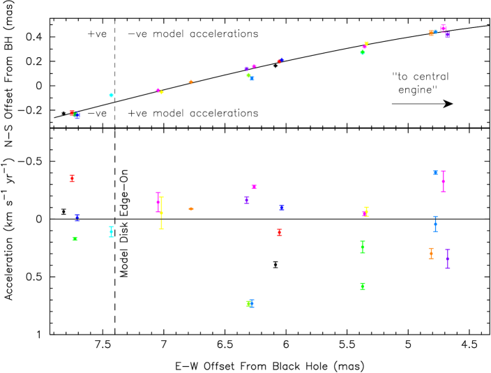
Figure 12: Sky positions and accelerations of fitted red-shifted maser components. (Lower Panel) LOS accelerations plotted as a function of disk east-west offset. The solid line marks zero LOS acceleration, which should occur when masers are on the disk midline. (Upper Panel) Sky positions of the corresponding maser components. The solid line indicates the disk midline predicted by the geometric model of Herrnstein et al. (2005). All maser positions Note that, for this model, masers above the model midline (upper panel) should also have negative accelerations at radii $<$ 7.4 mas, and positive accelerations at greater radii.

We can use the accelerations to confirm that the maser dynamic observables reflect real gas dynamics in the NGC 4258 accretion disk. The small accelerations of the high-velocity components suggest that they lie close to the disk midline. For this discussion, it is important to visualize the shape of the disk in the vicinity of the midline, which is in plane of the sky that includes the black hole. We show the geometry of the maser disk determined by Herrnstein et al. (2005) in Figure 10. On the midline, the disk shape is defined by the position angle warp, as shown in Figures 12 and 13 respectively for the red- and blue-side of the disk. That is, the expected midline curve is $y=r\cos\alpha_{r}$, where $y$ is the projected vertical position of the warped disk on the sky relative to the disk dynamical center in units of milli-arcseconds, $\alpha_{r}$ is the disk position angle measured North of East in the plane of the sky (the x-y plane in Figure 10) given by $\alpha_{r}=65.6$^∘$+5.04$^∘$r-0.22$^∘$r^{2}$ (Herrnstein et al., 2005), and where $r$ is the radial position of masers in the disk in mas. We take $r$ $\sim$$b$, where $b$ is the impact parameter in the plane of the sky measured from the disk dynamical center.

Over the radial range of emission from 4 to 8 mas on the red-side of the disk, the position angle varies from 84^∘ to 92^∘. The “tilt” of the disk at the midline is given by the inclination warp, which is described by $i_{r}=107$^∘$-2.29$^∘$r$ (Herrnstein et al., 2005). Hence, for the red side of the disk $i_{r}$ varies from 97^∘ at 4 mas, to 89^∘ at 8 mas. The range is the same for the blue-side of the disk. It is important to note that, at radii of 7.4 mas, we view the disk exactly edge on. Inside this radius, the near-side of the disk is tipped down with respect to the observer, while outside it is tipped up. Masers at radii smaller than 7.4 mas, that lie above the midline in VLBI images, should be behind the midline plane in the disk and have negative accelerations. Similarly masers beyond 7.4 mas radius, that appear above the midline in Figures 12 and 13, are expected to be in front of the midline plane and should have positive accelerations.

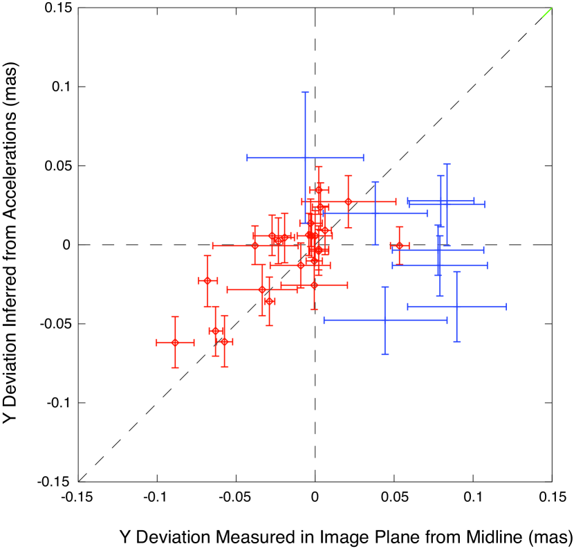
Figure 14: Vertical deviations from the warped disk of Herrnstein et al. (2005) calculated using acceleration data and VLBI data. See Section 6.1 for details.

We compared the vertical deviations in the VLBI image caused by the disk projection on the sky (see Figures 12 and 13), $y_{image}$, with the vertical deviations expected from the accelerations, $y_{acc}$. To derive $y_{acc}$ for each maser, we first computed its distance in the $z$-direction from the midline from its azimuth (which comes from its acceleration), that is $z=b\tan\phi$ where $\phi$ is the azimuth angle of the maser listed in Tables 2 and 3. From this azimuth offset, and the local slope of the warped disk at radius $r$, $y_{acc}$ was calculated as the projected offset from the midline. The plot of $y_{acc}$ vs. $y_{image}$ is shown in Figure 14. The errors in $y_{image}$ are the quadrature sum of the errors in the VLBI position and the errors in the midline definition. The errors in $y_{acc}$ are the result of acceleration measurement errors, inclination model errors, and errors due to a finite vertical distribution of masers. We adopt a disk thickness of 12 $\mu$as, the value determined from low-velocity emission in Paper I. The disk thickness corresponds to a temperature of about 600 K for hydrostatic equilibrium. In order to make the reduced $\chi^{2}$ of the fit equal 1, it was necessary to add a systematic r.m.s. acceleration of 0.1 km s^-1 yr^-1. Since the magnitude of the maser accelerations is up to $\sim$10 km s^-1 yr^-1, the systematic errors in the acceleration measurements are at the 1% level. The errors in Figure 14 reflect these contributions. Note that there is one significantly deviant point at 2.8$\sigma$ (the one at 1271 km s^-1 and $r=$7.37 mas).

6.2 Spiral Structure

Accelerations and positions of high-velocity emission can also be used to investigate theories of spiral structure in the accretion disk of NGC 4258. Firstly, Maoz (1995) noted periodic clustering of high-velocity component radii in a visual analysis of the single VLBI map by Miyoshi et al. (1995). Maoz inferred a characteristic wavelength of $\lambda_{char}=$0.75 mas (0.027 pc) for the clustering, and attributed it to spiral density waves that form by swing amplification. Spiral density waves can form in a disk that is unstable to non-axisymmetric perturbation in the 1$<Q\leq$2 regime, where $Q$ is the Toomre stability parameter (Toomre, 1964). Swing refers to the fact that a non-axisymmetric disturbance is converted to a trailing spiral arm (in which the outer tip points backwards, opposite the direction of disk rotation) due to shearing by differential rotation. Amplification occurs during this process, since the direction of the shear flow of the arm is the same direction as local epicyclic motions, which enhances the self-gravity of the arms. To satisfy this stability regime, Maoz (1995) required densities in spiral arms of n(H₂) = 10⁸ to 10¹⁰ cm^-3 which are sufficient to produce 22 GHz maser emission (e.g. Cooke & Elitzur, 1985), whilst those in the inter-arm regions are not. In the theory of Maoz (1995), masers are discrete physical clumps that can move freely through different spiral arms and can be tracked between epochs.

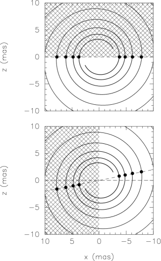
Figure 15: Comparison of spiral structure model predictions in the NGC 4258 accretion disk. (Upper) Schematic of maser disk according Maoz (1995). Masers (filled circles) are periodically located in density peaks of trailing spiral structures (represented here by a 2-arm logarithmic spiral). Accelerations are negative behind the midline (hatched area) and positive in front of the midline. Components should occur within several degrees of the midline for maximum velocity coherent maser path lengths. (Lower) Schematic of the maser disk according to MM98. Masers (filled circles) are periodically located in the disk, but offset from the midline by 2^∘ (note the angle is exaggerated here). Red-shifted high-velocity components have negative accelerations (hatched area), whereas blue-shifted component accelerations should be positive statistically-speaking. Maser emission occurs at the longest velocity coherent path lengths along the line-of-sight through spiral arms.

Maoz & McKee (1998, hereafter MM98) also propose that maser emission could arise behind spiral shocks in the NGC 4258 disk, from density and velocity coherence arguments. The shocks occur at the interface of spiral arms sweeping through the disk. In this case masers may not be discrete entities but a wave phenomenon, with emission arising at the tangents of the spiral shocks along the LOS, where the path length for amplification is highest. At different epochs, maser emission would not originate from the same gas condensations. The accelerations of the masers would no longer reflect pure Keplerian dynamics, as the action of the shock causes the excitation points for masers to move to greater radii in the disk. All maser velocities would shift to lower absolute values. This process would manifest itself observationally as positive accelerations for blue-shifted high-velocity components and as negative accelerations for red-shifted high-velocity components. Different spiral theories are schematically represented in Figure 15.

6.2.1 Spiral Density Wave Model (Maoz, 1995)

Maoz (1995) argues that (i) maser components are periodic in disk radius with a characteristic wavelength of $\lambda_{char}\sim$0.75 mas; and (ii) masers are located within several degrees of the disk midline. Point (ii) is required to avoid a wide range of accelerations of the masers due to spiral arms, which are not observed. If masers are near the midline, then the non-circular (peculiar) motion is largely perpendicular to the arms (Toomre, 1981) and perpendicular to the line-of-sight (and therefore undetectable in Doppler shifts). Maoz (1995) estimates that the component of the peculiar motion along the line-of-sight for high-velocity emission would not exceed 4.5 km s^-1, comparable to the measured accuracy of the Keplerian rotation curve (Maoz, 1995).

An apparent periodicity in the distribution of maser sky positions is obvious from VLBI images of the data. For formal quantification, we performed an analysis using the Lomb-Scargle periodogram for the 18 epochs of VLBI data described in Paper I. First, we created a “binary” dataset from the VLBI positions, in which any disk position that had detected emission was assigned a “flux density” of “1”, to ensure that disparity in flux density between red and blue-shifted emission did not affect the outcome of the analysis. We gridded the binary dataset at intervals of 0.005 mas, i.e., on scales much shorter than any expected $\lambda_{char}$, and placed zeroes at positions at which we did not detect, emission in the VLBI maps. Using the periodogram, we found a dominant period in the binary distribution of high-velocity maser positions of 0.75 mas (Figure 16), at the same value as that estimated by (Maoz, 1995). We also predicted that emission should exist at a velocity of about $-$330 km s^-1 in the blue-shifted spectrum. In subsequent observations obtained with the GBT on 2003 October 23, the emission predicted by the periodogram analysis was detected at $-$329 km s^-1. At $<$10 mJy, this emission would not have been detected in our VLBI observations.

We note that the model of Maoz (1995) has densities in the spiral arms that can produce maser emission, but not in the inter-arm regions. In the denser spiral arms, gas condensations naturally form. In this event, discrete maser-emitting condensations could be tracked as they move across an arm. They are not necessarily persistent in the inter-arm region, i.e. discrete maser condensations may only exist within arms and disperse in the inter-arm regions. As a result, clumps responsible for low-velocity emission do not survive to beam high-velocity emission toward the observer after one quarter of a rotation, and conversely, high-velocity clumps do not survive to eventually be seen as low-velocity clumps.

6.2.2 Spiral Shock Model (MM98)

The specific predictions of MM98 for masers, in addition to periodicity in maser sky positions, are that (i) blue-shifted components are accelerating and they are located behind the disk midline, and (ii) red-shifted components are decelerating and should be located in front of the midline. By contrast, in a disk dominated by Keplerian dynamics, masers in front of the midline should have a positive sign of acceleration, and masers located behind the midline should have a negative sign of acceleration.

We do not find that the accelerations of high-velocity components conform to the MM98 model. Both the red- and blue-shifted component accelerations are statistically near zero (see Section 4.1 and Tables 2 and 3), although there is a 2.6$\sigma$ bias of the latter to negative accelerations which is not in agreement with predictions of MM98. We note that Yamauchi et al. (2005) presented evidence in support of MM98. However, Yamauchi et al. (2005) measured the acceleration of one blue-shifted component only, which had a positive acceleration at the 2$\sigma$ significance level. We obtain a negative acceleration for the same component (see Section 5) when it is decomposed into 3 features. Of the eight blue-shifted components for which we measured accelerations, only one is positive. Bragg et al. (2000) also does not find accelerations that would support the MM98 theory.

6.2.3 Other Origins for the Periodicity

We also considered the possibility that orbiting objects (e.g., stars) create the sub-structure in the NGC 4258 accretion disk, with for example some resonance mechanism causing regularity in the spacings. If the stellar density is the same in the central regions of NGC 4258 as in the center of the Milky Way, then integrating $\rho_{*}(R)=1.2\times 10^{6}(R/0.425)^{-\alpha}$ between $R=$0.14 and 0.28 pc and assuming $\alpha$=1.4 (from Genzel et al., 2003) yields a stellar mass of 2$\times$10⁴ M_⊙ in the spherical volume containing the maser disk, so there are likely at least several thousand stars. The cumulative effect of many passages of stars around the black hole might bring them into a circular orbit co-rotating with the disk, although we note that highly eccentric stellar orbits are found in our Galactic Center. Each star could then either open up a gap in the disk (if the disk is thinner than the star’s Hill radius and the viscosity in the disk is sufficiently low) or accrete material from the disk. The vertical thickness of the maser disk is measured to be 12 $\mu$as (Paper I). We therefore estimate the lower limit on the mass of a star (or stellar cluster) required to create a gap completely through the disk to be $>$ 0.05 M_⊙ ($2r_{Hill}\approx 2r_{orb}(m_{*}/3M_{bh})^{1/3}=0.0003$ pc for $\overline{r_{orb}}$=0.2 pc), such that any star, even a brown dwarf, could create a gap in the disk equal to its thickness. We note that a number of massive He I stars (of mass 30 to 100 M_⊙) exist between 0.04 to 0.5 pc (1^′′ to 12^′′) of the Galactic center (Genzel et al., 2003), and that a corresponding $\sim$100 M_⊙ star in the NGC 4258 disk would create a gap of $2r_{hill/roche}$=0.006 pc. The stars would be at radii several orders of magnitude greater distances from the SMBH than their tidal disruption radii $r_{tidal}\simeq r_{*}(M_{bh}/m_{*})^{1/3}$, where $r_{*}$ and m_∗ are the radius and mass of the star respectively (see e.g, Bogdanović et al., 2004).

7 Implications for the Accretion Disk from Low-Velocity Emission

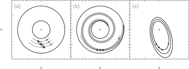
Figure 18: Scenarios for producing the trend in line-of-sight accelerations of low-velocity emission as a function of component Doppler velocity. The line-of-sight direction is along the $z$-axis. (a) Masers in circular, Keplerian orbits with locations determined by disk geometry and orientation. In this scenario, components (shown as filled, black circles) are in circular orbits about the black hole (black cross) but only produce visible maser action within a favorable locus of disk radius and azimuth angle (shown in gray) determined by the warping of the disk and tangency of the line of sight to the disk. The acceleration trend in this case is due to emission from a number of different maser components in orbits of different radii. (b) Masers in a circular, Keplerian orbit that crosses a spiral arm. In this scenario, maser components are in a circular orbit about the black hole and encounter a spiral arm that perturbs the orbital motions (the arm is represented here by a gray logarithmic spiral, but a more realistic scenario would be fragmentary, as in flocculent spiral galaxy disks.) The acceleration trend in this case is due to the passage of maser components through a spiral arm of lower pattern speed than the local Keplerian velocity (see Figure 19). (c) Masers in non-circular, confocal, Keplerian orbits. Maser components in the same elliptical orbit by definition are at different radii and exhibit different accelerations, but they may instead lie on different orbits, with the same effect.

The range of accelerations measured for low-velocity components is consistent with the warped disk model of Herrnstein et al. (2005) (see our Figures 10 and 11). However, the systematic trend in component acceleration with Doppler velocity (see Section 4.2) is not predicted by this model. The trend is likely connected to some aspect of the warped disk geometry that results in a preferred locus in disk radius and azimuth angle within which low-velocity maser action is favored (Figure 18a) as a result of geometry and orientation to the line of sight, and we investigate this point more in the next paper of this series, in which we report new modeling of the 3D disk structure and dynamics based on the expanded dataset presented in Paper I and in this paper. In order to understand other types of “higher-order” phenomena that could give rise to the trend however, we attempted to reproduce the observations by (i) assuming circular orbits in the disk with a spiral arm in the low-velocity maser region (Figure 18b) and (ii) allowing for eccentricity in maser orbits (Figure 18c). In the preliminary investigations that follow, we have assumed that the maser disk is flat and is viewed edge-on.

7.1 Spiral Structure

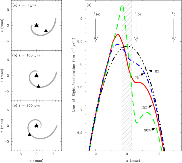
Figure 19: The effect of a spiral arm on accelerations of low-velocity masers in the NGC 4258 disk.(a) Initial conditions for an N-body simulation of a maser clump (black triangle) orbiting a supermassive black hole of $3.8\times 10^{7}$ $M_{\odot}$ (Herrnstein et al., 2005) (black star). The parameters of the trailing logarithmic spiral arm (grey), represented by 8000 particles, were arbitrarily chosen to be r₀ = 1.5 mas, $b$=0.42 and $\phi_{0}$ = 0^∘ , where $r=r_{0}\exp(b(\phi-\phi_{0}))$. The pattern speed of the spiral arm is half that of the Keplerian orbital velocity at any given radius. Note that the true breadth of the arm (10^-2 pc) is exaggerated for clarity. (b) Snapshot at t = 100 years. (c) Snapshot at t = 200 years. (d) Maser component line-of-sight acceleration as a function of disk impact parameter due to both the supermassive black hole and a spiral arm of varying masses. Arm mass is quoted as a percentage of the upper limit maser disk mass, M_disk,upper = 9 $\times$ 10⁵ M_⊙ (Herrnstein et al., 2005). Note the significant deviation of the acceleration profiles at 7, 15 and 30% from that of the 0% (black hole only) sinusoid. The curve that best matches observations is that for an arm mass of 15%. The grey hatched area indicates the observed projected extent in disk impact parameter of the low velocity masers.

In order to investigate whether spiral structure could give rise to the gradient evident in accelerations of low-velocity components with Doppler velocity, we performed $N$-body simulations for a maser orbiting a supermassive black hole ($3.8\times 10^{7}$ M_⊙; Herrnstein et al., 2005) in a flat disk, and encountering a spiral arm of various masses (Figure 19). For the simulations, we used a direct $N$-body integration code, NBODY0 (Aarseth, 1985), in which each particle is followed with its own integration step to account for a range of dynamical rates. See Aarseth (1985) for more details.

We represented a spiral arm at $t=$0 (Figure 19a) using 8000 particles distributed along an arbitrarily-chosen trailing logarithmic spiral arm of $r=r_{0}\exp[\,b(\phi-\phi_{0})\,]$, in which $b=$0.42, $\phi_{0}=$0^∘ and $r_{0}=$ 1.5 mas or 0.06 pc, with a radial extent of 10^-2 pc. The pattern speed of the arm was set to be half that of the Keplerian orbital velocity (by reducing the force on arm particles by a factor of 4) at any given radius, and gravitational interaction between arm particles was ignored. We based values for the fractional radial extent and pattern speed of the arm roughly on those of Galactic spiral arms. To avoid potentially infinite acceleration between arm particles and the maser, and to better represent a smooth distribution of mass in the arm, we included a “softening” term of $5\times 10^{-3}$ pc that was added in quadrature to each maser-particle separation.

We varied the mass contained in the arm (bounded by the upper mass limit for the maser disk determined by Herrnstein et al. (2005) of M${}_{disk,upper}=$9$\times$10⁵ M_⊙) for different runs of the code. For any given run, we followed the evolution of a maser cloud through the spiral arm (Figure 19a-c) for several hundred years, sampling every 0.55 years.

The computed line-of-sight accelerations for the maser showed significant deviations from that of a mass-less arm, for arm masses greater than a few percent level of M_disk,upper (Figure 19d). We found the “amplitude” of the acceleration deviation to be directly proportional to arm mass and could reproduce observed trends in acceleration (see Section 4.2) for an arm mass of 15% of the upper limit maser disk mass. In the simulations, the acceleration trend is reproduced when the maser is “in” the spiral arm (between 100 and 200 years in Figure 19) We note that our calculations include gravitational effects only and do not attempt to incorporate shocks or magneto-hydrodynamic effects of spiral density wave theory.

7.2 Eccentric Accretion Flows

While accretion flows are generally believed to circularize on timescales much shorter than the viscous timescale, Statler (2001) showed that elliptical orbits of $e$ $\leq$ 0.3 can be long-lived if the disk is thin, and if the orbits are nested and confocal, with precession rates that maintain the alignment.

We describe a system of nested elliptical orbits of identical eccentricity, $e$, of differing semi-major axes, $a_{semi}$, and with the same periapsis angle, $\omega$, about a supermassive black hole. The periapsis angle is defined here as the angle between the sky plane to the periastron point on each orbit (increasing from the “red-shifted” midline in the sense of disk rotation). In the discussion that follows, it is important to note that no matter the $e$ and $\omega$ of the system, red-shifted high-velocity maser emission components must originate from an azimuthal angle of $\phi$ $\approx$ 0^∘(where $\phi-\omega$ is the angle of the component from periastron), and blue-shifted components from $\phi$ $\approx$ 180^∘on the basis of velocity coherence and acceleration arguments.

We first used the symmetry of the position-velocity (P-V) diagram of high-velocity emission to place limits on eccentricity. At any given radius in the disk in the plane of the sky (i.e., where the radial orbital velocity component is perpendicular to the LOS), the Doppler velocity is given by

$$v_{los}=\left(\frac{GM}{r}\right)^{1/2}\left[1+e\cos(\phi-\omega)\right]^{1/2}\cos\phi+v_{sys}$$ (1)

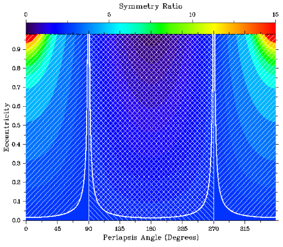
Figure 20: Contour plot of the “symmetry” ratio ($v_{red,\,los}/v_{blue,\,los}$) of model P-V diagrams for eccentricity ($e$) as a function of periapsis angle ($\omega$). The symmetry of the data eliminates values of $e$ and $\omega$ in the positive-gradient hatched regions of the plot. Using acceleration data for low-velocity emission, we further eliminate all of the negative-gradient hatched region of 90^∘ $\leq$ $\omega$ $\leq$ 270^∘ for low-velocity maser components on the same orbit. Only unhatched regions of parameter space are permitted by our dataset.

where $r$ is angular radius in the disk and $M=M_{BH}/D$. We can therefore compute the ratio of $v_{red,\,los}/v_{blue,\,los}$ for closed orbit ($e$ $<$ 1) values of $e$ and $\omega$ using $\phi$=0^∘ for the red-shifted high-velocity emission and $\phi$=180^∘ for the blue-shifted high-velocity emission. Note that this ratio is always unity for circular orbits ($e=$ 0) and for orbits of any eccentricity viewed along the semi-major axes i.e., for $\omega$=90^∘ or 270^∘ in our definition. Using values of v_sys=472$\pm$4 km s^-1 (Cecil et al., 1992) and a disk dynamical center position of $x_{0}$ = $-$0.1$\pm$0.1 mas estimated from jet continuum data (Herrnstein, 1997) within the 1$\sigma$ uncertainties (noting that, by allowing a 1$\sigma$ deviation in each quantity we are actually using a combined uncertainty $>$1$\sigma$), we computed the observed ratio of $v_{red,\,los}/v_{blue,\,los}$ from our VLBI data to lie between 0.98 to 1.03. This constrains maser orbits to have either a low eccentricity of $<$0.05 or to be more highly-eccentric but viewed (nearly) along the semi-major axes of the orbits ($\omega$=90^∘ or 270^∘). The parameter space we eliminate using the P-V diagram is marked by the white hatching of positive gradient in Figure 20.

To constrain the eccentricity and periapsis angle further, we can also use the low-velocity acceleration data as a function of Doppler velocity. Instantaneous acceleration is given by $\dot{v}_{los}=-(GM/r^{2})\sin\phi$ and $r=a_{semi}(1-e^{2})/(1+e\cos(\phi-\omega))$ so we can write

$$\frac{d\dot{v}_{los}}{dv_{los}}=\left[\frac{GM}{(1-e^{2})^{4}a_{semi}^{3}}\right]^{\frac{1}{2}}\frac{\gamma^{2}\cos\phi-2\gamma e\sin(\phi-\omega)\sin\gamma}{\sin\phi}$$ (2)

where $\gamma=1+e\cos(\phi-\omega)$ and where we assume that low-velocity masers occupy the same orbit such that $a_{semi}$ is a constant, implied by the restriction of low-velocity masers to a narrow portion of the P-V diagram. Using the sign of the gradient, we can further exclude all periapsis angles of 90^∘ $\leq$ $\omega$ $\leq$ 270^∘ , marked by the white hatching of negative gradient in Figure 20. Since the $e$ - $\omega$ parameter space remaining after these eliminations is very small (regions with no hatching at all in Figure 20), it is unlikely that the maser orbits are highly eccentric and observed along a special viewpoint. However, this is a topic we revisit in the next paper of this series, in which we perform 3D accretion disk modeling of the masers including eccentric maser orbits.

8 Conclusions

In this paper, we measured centripetal accelerations of maser spectral components for data spanning 1994 to 2004. We found that high-velocity emission accelerations lie in the range $-$0.7 to $+$0.7 km s^-1 yr^-1, indicating the emission originates within 13^∘ of the disk midline for material in Keplerian rotation (see Tables 2 and 3). The good agreement of maser projected vertical positions ($y$-positions) of high-velocity emission derived from the acceleration data, with those of VLBI images, confirms that masers trace true gas dynamics of the disk. While the high-velocity accelerations do not support the MM98 model of trailing shocks associated with spiral arms in the disk, we find a spatial periodicity in high-velocity emission of wavelength 0.75 mas. This supports the model of Maoz (1995) of spiral structure due to density waves in the disk.

We measured accelerations of low-velocity emission in the range 7.7 to 8.9 km s^-1 yr^-1, which is consistent with emission that originates from a concavity in the front-side of the disk reported by Herrnstein et al. (2005). We confirm a systematic trend in accelerations of low-velocity emission as a function of component Doppler velocity, found by Haschick et al. (1994) and Greenhill et al. (1995b). Preliminary investigations into the origin of the trend suggest that eccentricity in maser orbits is unlikely to be the cause. The trend may be caused either by the effect of a stationary or slowly moving spiral arm, or by a disk feature which causes a stationary pattern of radius versus azimuth angle.

We are grateful to Maryam Modjaz and Paul Kondratko for providing their GBT data. We thank Alar Toomre for helpful discussions.

Table 1: The Dataset.

——– Epoch ——–			Observations		Observing Details		Comments
No.	Date	Day	Program	Telescope	$\Delta$v	Sensitivity
		No.	Code		(km s-1)	(mJy)
1	1994 Apr 19	0	BM19	VLBA	0.21	43	Systemic, red and blue-shifted emission
2	1995 Jan 07	263	AG448	VLA-CD	0.33	25	Systemic, red and blue-shifted emission
3	1995 Jan 08	264	BM36a	VLBA	0.21	80	Systemic, red and blue-shifted emission
4	1995 Feb 23	310	AG448	VLA-D	0.33	25	Systemic, red and blue-shifted emission
5	1995 Mar 16	331	$\cdots$	EFLS	0.33	85	Red-Shifted emission only
6	1995 Mar 24	339	$\cdots$	EFLS	0.33	90	Red-Shifted emission only
7	1995 Mar 25	340	$\cdots$	EFLS	0.33	95	Red-Shifted emission only
8	1995 Apr 04	350	$\cdots$	EFLS	0.33	85	Red-Shifted emission only
9	1995 Apr 20	366	AG448	VLA-D	0.33	20	Systemic, red and blue-shifted emission
10	1995 May 29	405	BM36b	VLBA	0.21	30	Systemic, red and blue-shifted emission
11	1995 Jun 08	415	AG448	VLA-AD	0.33	20	Systemic, red and blue-shifted emission
12	1995 Jun 25	432	$\cdots$	EFLS	0.33	110	Red-Shifted emission only
13	1995 Jul 29	466	AG448	VLA-A	0.33	$\cdots$	No data
14	1995 Sep 09	508	AG448	VLA-AB	0.33	$\cdots$	No data
15	1995 Nov 09	569	AG448	VLA-B	0.33	37-60	Systemic, red and blue-shifted emission
16	1996 Jan 11	632	AG448	VLA-BC	0.33	20	Systemic, red and blue-shifted emission
17	1996 Feb 22	674	BM56a	VLBA	0.21	25	Systemic, red and blue-shifted emission
18	1996 Feb 26	678	AG448	VLA-C	0.33	23-30	Systemic, red and blue-shifted emission
19	1996 Mar 29	710	AG448	VLA-C	0.33	20	Systemic, red and blue-shifted emission
20	1996 May 10	752	AG448	VLA-CD	0.33	15-24	Systemic, red and blue-shifted emission
21	1996 Jun 27	799	AG448	VLA-D	0.33	$\cdots$	No data
22	1996 Aug 12	846	AG448	VLA-D	0.33	23-36	Systemic, red and blue-shifted emission
23	1996 Sep 21	886	BM56b	VLBA	0.21	20	High-velocity emission only
24	1996 Oct 03	898	AG448	VLA-AD	0.33	50	Systemic, red and blue-shifted emission
25	1996 Nov 21	947	AG448	VLA-A	0.33	21-26	Systemic and red-shifted emission
26	1997 Jan 20	1007	AG448	VLA-AB	0.33	27-37	Systemic and red-shifted emission
27	1997 Feb 10	1028	AG448	VLA-AB	0.33	17-23	Systemic and red-shifted emission
28	1997 Mar 06	1052	BM56c	VLBA	0.21	4.7	Systemic, red and blue-shifted emission
29	1997 Oct 01	1261	BM81a	VLBA	0.21	4.1	Systemic, red and blue-shifted emission
30	1998 Jan 27	1379	BM81b	VLBA	0.21	5.0	Systemic, red and blue-shifted emission
31	1998 Sep 05	1600	BM112a	VLBA	0.21	4.6	Systemic, red and blue-shifted emission
32	1998 Oct 18	1643	BM112b	VLBA	0.42	4.6	Systemic and red-shifted emission
33	1998 Nov 16	1672	BM112c	VLBA	0.42	4.4	Systemic and blue-shifted emission
34	1998 Dec 24	1710	BM112d	VLBA	0.42	$\cdots$	No data
35	1999 Jan 28	1745	BM112e	VLBA	0.42	4.8	Systemic and blue-shifted emission
36	1999 Mar 19	1795	BM112f	VLBA	0.42	4.5	Systemic and red-shifted emission
37	1999 May 18	1855	BM112g	VLBA	0.42	5.2	Systemic and blue-shifted emission
38	1999 May 26	1863	BM112h	VLBA	0.21	3.5	Systemic, red and blue-shifted emission
39	1999 Jul 15	1913	BM112i	VLBA	0.42	$\cdots$	No data
40	1999 Sep 15	1975	BM112j	VLBA	0.42	6.3	Systemic and blue-shifted emission
41	1999 Oct 29	2019	BM112k	VLBA	0.42	4.7	Systemic and blue-shifted emission
42	2000 Jan 07	2089	BM112l	VLBA	0.42	3.9	Systemic and blue-shifted emission
43	2000 Jan 30	2112	BM112m	VLBA	0.42	4.7	Systemic and red-shifted emission
44	2000 Mar 04	2146	BM112n	VLBA	0.42	4.3	Systemic and blue-shifted emission
45	2000 Apr 12	2185	BM112o	VLBA	0.42	5.5	Systemic and red-shifted emission
46	2000 May 04	2207	BM112p	VLBA	0.42	5.0	Systemic and blue-shifted emission
47	2000 Aug 12	2307	BG107	VLBA	0.42	7.2	Systemic, red and blue-shifted emission
48	2003 Apr 10	3298	$\cdots$	GBT	0.21	2.9	Systemic, red and blue-shifted emission
49	2003 Oct 23	3474	$\cdots$	GBT	0.21	2.9	Systemic, red and blue-shifted emission
50	2003 Dec 08	3520	$\cdots$	GBT	0.21	2.9	Systemic, red and blue-shifted emission
51	2004 May 21	3685	AH847	VLA	0.21	20	Portions of red-shifted spectrum

Table 2: Fitted Accelerations For Red-Shifted High-Velocity Doppler Components.

————– Component ————–			——— Epochs ———		Time-Averaged	Component
No.	Velocity	Acceleration	No. in Fit	Time Baseline	Azimuth Angle	Radius
	(km s-1)	(km s-1 yr-1)		(yr)	(deg)	(pc)
1	1248.14$\pm$0.02	-0.06 $\pm$0.02	24	6.0	-1.6$\pm$0.6	0.28
2	1250.80$\pm$0.03	-0.35 $\pm$0.03	24	6.0	-8.9$\pm$0.8	0.28
3	1252.24$\pm$0.01	0.17 $\pm$0.01	24	6.0	4.3$\pm$0.3	0.28
4	1254.34$\pm$0.02	-0.01 $\pm$0.03	24	6.0	-0.3$\pm$0.7	0.28
5	1270.89$\pm$0.05	0.11 $\pm$0.04	24	6.0	2.5$\pm$1.0	0.27
6	1282.21$\pm$0.06	-0.15 $\pm$0.08	4	0.7	-3.1$\pm$1.8	0.26
7	1283.87$\pm$0.08	-0.05 $\pm$0.14	4	0.7	-1.1$\pm$3.0	0.26
8	1309.08$\pm$0.01	-0.09 $\pm$0.01	30	9.0	-1.7$\pm$0.1	0.24
9	1328.64$\pm$0.04	0.73 $\pm$0.02	29	5.3	12.6$\pm$0.6	0.23
10	1330.73$\pm$0.06	0.73 $\pm$0.03	29	5.3	12.4$\pm$0.7	0.23
11	1337.36$\pm$0.04	-0.16 $\pm$0.03	35	6.3	-2.7$\pm$0.5	0.23
12	1339.58$\pm$0.01	-0.28 $\pm$0.01	35	6.3	-4.6$\pm$0.3	0.22
13	1351.00$\pm$0.03	0.40 $\pm$0.03	34	6.0	6.1$\pm$0.5	0.22
14	1353.85$\pm$0.03	0.11 $\pm$0.03	34	6.0	1.8$\pm$0.4	0.22
15	1355.56$\pm$0.02	-0.10 $\pm$0.02	34	6.0	-1.5$\pm$0.3	0.22
16	1395.59$\pm$0.09	0.24 $\pm$0.05	21	4.3	3.1$\pm$0.7	0.20
17	1398.09$\pm$0.05	0.58 $\pm$0.03	21	4.3	7.3$\pm$0.4	0.20
18	1403.60$\pm$0.01	-0.05 $\pm$0.02	34	6.0	-0.6$\pm$0.2	0.19
19	1406.74$\pm$0.05	-0.06 $\pm$0.04	34	6.0	-0.8$\pm$0.5	0.19
20	1449.43$\pm$0.04	0.30 $\pm$0.04	25	2.9	3.0$\pm$0.5	0.18
21	1452.35$\pm$0.01	-0.40 $\pm$0.02	25	2.9	-4.0$\pm$0.2	0.18
22	1452.80$\pm$0.14	0.04 $\pm$0.06	25	2.9	0.4$\pm$0.6	0.18
23	1455.26$\pm$0.19	-0.33 $\pm$0.09	25	2.9	-3.2$\pm$0.9	0.17
24	1468.08$\pm$0.07	0.34 $\pm$0.08	4	2.6	3.2$\pm$0.8	0.17
Mean Acceleration:		0.02 $\pm$0.06	Mean Azimuth Angle:		0.2$\pm$3.6

Table 3: Fitted Accelerations For Blue-Shifted High-Velocity Doppler Components.

————– Component ————–			——— Epochs ———		Time-Averaged	Component
No.	Velocity	Acceleration	No. in Fit	Time Baseline	Azimuth Angle	Radius
	(km s-1)	(km s-1 yr-1)		(yr)	(deg)	(pc)
1	-282.21$\pm$0.07	-0.47 $\pm$0.10	6	1.5	-13.2$\pm$2.9	0.29
2	-284.00$\pm$0.06	-0.12 $\pm$0.08	6	1.5	-3.3$\pm$2.3	0.29
3	-286.05$\pm$0.13	-0.38 $\pm$0.13	6	1.5	-10.3$\pm$3.5	0.29
4	-374.20$\pm$0.05	-0.32 $\pm$0.26	5	1.1	-5.6$\pm$4.7	0.23
5	-375.78$\pm$0.22	-0.72 $\pm$0.49	5	1.1	-12.6$\pm$ 8.6	0.23
6	-435.00$\pm$0.03	-0.29 $\pm$0.05	16	3.5	-3.9$\pm$ 0.7	0.20
7	-439.97$\pm$0.02	+0.04 $\pm$0.04	15	2.9	0.5$\pm$ 0.5	0.20
8	-514.48$\pm$0.04	-0.24 $\pm$0.16	4	0.5	-2.3$\pm$ 1.5	0.17
Mean Acceleration:		-0.21 $\pm$0.08	Mean Azimuth Angle:		-3.3$\pm$6.9

Table 4: Accelerations for Low-Velocity Maser Doppler Components.

Velocity	Acceleration	Radius in Geometric Model
(km s-1)	(km s-1 yr-1)	(mas)
438	7.65$\pm$0.15	4.20$\pm$0.04
448	7.81$\pm$0.13	4.16$\pm$0.03
458	7.85$\pm$0.13	4.15$\pm$0.03
468	7.77$\pm$0.08	4.17$\pm$0.02
478	7.84$\pm$0.17	4.15$\pm$0.04
488	8.29$\pm$0.12	4.04$\pm$0.03
498	8.16$\pm$0.13	4.07$\pm$0.03
508	8.09$\pm$0.09	4.09$\pm$0.02
518	8.75$\pm$0.09	3.93$\pm$0.02
528	8.55$\pm$0.06	3.97$\pm$0.02
538	8.36$\pm$0.10	4.02$\pm$0.02
548	8.87$\pm$0.27	3.89$\pm$0.05

Table 5: Studies of Acceleration Among NGC 4258 Maser Components

Study	Antennas	Sensitivity	Dates	Velocity	Components	Acceleration
		(mJy)		Range	Tracked	Range
				(km s-1)		(km s-1 yr-1)
Haschick & Baan (1990)	HAYS	55$-$70	7/1986$-$11/1989	340 to 590	1 (systemic)	10
			$\approx$ monthly
Haschick et al. (1994)	HAYS	30$-$55	7/1986$-$11/1993	340 to 590	4 (systemic)	6.2$-$10.4
			$\approx$ monthly
Greenhill et al. (1995b)	EFLS	30	10/1984$-$12/1986	335 to 665	12	8.1$-$10.9
			every few days $-$ months	1185 to 1515	20	$<$$\pm$1
			02/1993$-$03/1994	$-$570 to $-$240	3	$<$$\pm$1
			more frequently
Nakai et al. (1995)	NRO	13$-$20	1992	$-$1197 to 2664	13 (systemic)	7.2$-$11.1
			$\approx$ weekly	$\cdots$	8 (red)	$<$$\pm$0.7
				$\cdots$	1 (blue)
Herrnstein et al. (1999)	VLBA+VLA (3 epochs)	6$-$12	04/1994$-$02/1996	430 to 590	30 (systemic)	6.8$-$11.6
	VLBA+VLA+GB (1 epoch)			1225 to 1490	1 (red)	0.0
				$-$450 to $-$350	0 (blue
Bragg et al. (2000)	VLBA (5 epochs)	40	04/1994$-$02/1997	390 to 660	12 (systemic)	7.5$-$10.4
	EFLS (5 epochs)	95		1235 to 1460	17 (red)	-0.77$-$0.38
	VLA (17 epochs)	20		$-$460 to $-$420,$-$390 to $-$350	2 (blue)	-0.41,$+$0.04
Yamauchi et al. (2005)	NRO	8$-$140	01/1992$-$04/2005	$-$725 to 1720	14 (red)	-0.52$-$0.41
			30 irregularly spaced spectra	$\cdots$	1 (blue)	+0.2
				$\cdots$
This Work	Bragg Dataset(27 epochs)	20$-$95	04/1994$-$05/2004	-850 to 1850	25 (systemic)	6.1$-$10.8
	VLBA+VLA+EFLS (18 epochs)	3.2$-$7.8	on average every 2.5 months	$\cdots$	24 (red)	-0.4$-$0.7
	GBT(3 epochs)	a few mJy		$\cdots$	8 (blue)	-0.7$-$0.04
	VLA(1 epoch)	5

Figure 1: (a) Sky positions for 22 GHz maser emission in NGC 4258 obtained using VLBI on 18 epochs from 1997 March 06 to 2000 August 12 described in Paper I. Red-shifted high-velocity emission occurs from 3 to 8 mas in the disk; low-velocity emission occurs in the range -1 to 1 mas and blue-shifted high-velocity emission in the range 5 to 9 mas. Note that $(0,0)$ in the plot does not represent the disk dynamical center. (b) GBT spectrum of red-shifted high-velocity emission from Modjaz et al. (2005), obtained on 2003 October 23. The 1$\sigma$ noise in the spectrum is 1.6 mJy. The arrow marks weak, newly-detected emission at 1652 km s^-1 (Paper I). (c) GBT spectrum of low-velocity maser emission. The arrows mark emission extrema. The dotted line denotes the galactic systemic velocity of 472 km s^-1 (Cecil et al., 1992). (d) GBT spectrum of blue-shifted maser emission.

Figure 2: (a) Velocity vs. time plot for systemic components using data from 1998 January 27 to 2000 August 12 during which sampling was every $\sim$3 months. Drifts in Doppler velocities of strong components are clearly evident and consistent with centripetal accelerations. The dashed line marks the galactic systemic velocity of 472 km s^-1. (b) Corresponding plot for red-shifted components. Small magnitudes of drifts in component Doppler velocities are consistent with near-zero observed accelerations for components near the disk midline.

Figure 3: Example of a simultaneous 4-Gaussian function fit to a blend of red-shifted components over 25 epochs (2.9 years). Filled circles mark the data points. Residuals are plotted with 1$\sigma$ errorbars. Model Gaussian functions are shown in solid black lines. The epoch day number is marked in the upper right of each panel. Table 1 lists the corresponding dates.

Figure 4: As for Figure 3, but for a blue-shifted high-velocity emission blend.

Figure 5: Example of Gaussian decomposition for low-velocity emission. A velocity-portion of a fit over 9 epochs is shown, in which dots are data and black symbols are the residuals including 1$\sigma$ error bars. Individual model Gaussians are coded using the same color at each epoch, such that Doppler velocity drifts are clearly evident. Numbers in the upper right corner of each panel are the number of days since 1994 April 19.

Figure 6: Results of Gaussian decomposition for low-velocity emission. (a) Measured accelerations from each of the four time-consecutive 9-epoch fits. Each fit required $\sim$55 Gaussian components. The line-of-best-fit to all the data is shown. (b) Data in (a) binned into 10 km s^-1 intervals. The errorbars are the standard deviation of the mean in each bin.

Figure 7: Predicted position-velocity diagram for a linear fit to the low-velocity acceleration data (see Figure 6). Symbols mark observed data from the 18 VLBI epochs of Paper I, binned into 0.05 mas intervals. The curve shows the diagram predicted from the line-of-best-fit to the acceleration data. Curve and data are in close correspondence except at three most positive values of impact parameter.

Figure 8: Comparison of acceleration measurements for red-shifted maser spectral components: the current work (black circles); Bragg et al. (2000) (red triangles); Yamauchi et al. (2005) 1997 to 2005 (green squares); Yamauchi et al. (2005) 1992 to 2005 (blue stars). Yamauchi et al. (2005) derive accelerations from their dataset over two time ranges, one of which is a subset of the other. All velocities have been converted to a relativistic definition, are referenced to the LSR, and have been adjusted to a common reference date (our monitoring day 2000). Measurements from the different studies are in broad agreement, however this work tends to identify more components in any given blend compared with earlier work.

Figure 9: Comparison of acceleration measurements for low-velocity maser spectral components. All studies are plotted at the mid-date of their monitoring period, in order of increasing mid-date. Only components for which sufficient velocity drift data were obtained have been plotted here. The majority of studies show a trend of increasing acceleration as a function of Doppler velocity. We note that the present work is represented by binned data here, whereas other studies display measurements for individual components. The uncertainties plotted for the binned values are the standard deviation of the mean of each bin, as for Figure 6b. For comparison, in the present work we measure accelerations for $\sim$55 components in the low-velocity spectrum.

Figure 10: Best-fitting maser disk from Herrnstein et al. (2005) viewed from [-40,40,-50]. The line-of-sight is shown as a line extending beyond the outer edge of the disk in black along the $z$-direction. Solid color contours show disk elevation, where red is the maxmium and dark blue is the minimum. The disk midline for $\phi$=0^∘ and 180^∘ is shown for red-shifted emission (red line) and blue-shifted emission (blue line) respectively. Low-velocity (systemic) masers lie in the concavity on the front side of the disk.

Figure 11: Location of the low-velocity emission in the concavity (Herrnstein et al., 2005). Isovelocity contours are marked in color and are in units of km s^-1 relative to v_sys km s^-1 (Herrnstein et al., 2005). The LOS is along the $z$-direction, and therefore a vertical contour would mark a zero velocity gradient in the line-of-sight. The black line marks the bottom of the concavity. The black symbols mark the position of the low velocity emission, derived from the acceleration data. Observer views along the $z$-axis.

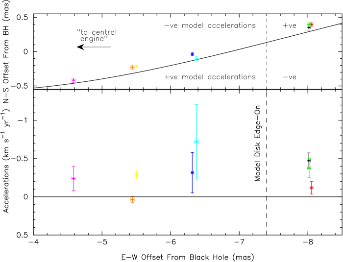
Figure 13: As for Figure 12, but for fitted blue-shifted high-velocity components. For this model, masers above the model midline (upper panel) should have negative accelerations at radii $<$ 7.4 mas, and positive accelerations at greater radii.

Figure 16: Periodogram of the positions of the high-velocity components in the NGC 4258 disk. The dominant frequency peak at 1.33 mas^-1 corresponds to a characteristic wavelength of 0.75 mas. The dashed horizontal black line marks the 3$\sigma$ significance level. We confined our analysis to “wavelengths” of $<$ 2 mas, since longer periods would not be well-constrained by our dataset.

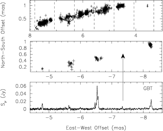
Figure 17: (Top) Sky positions of red-shifted high-velocity emission in the NGC 4258 disk obtained using VLBI over 18 epochs. Dashed lines mark nodes at characteristic wavelengths of 0.75 mas, proposed by Maoz (1995). (Middle) Blue-shifted components in the NGC 4258 disk. (Bottom) GBT spectrum of the blue-shifted high-velocity emission taken on 2003 October 23. Velocity has been represented as approximate east-west offset using offset . The arrow marks the velocity of the “missing” blue component predicted by the Fourier analysis and detected independently in the spectrum.

References

- Aarseth (1985) Aarseth, S. J. 1985, in IAU Symposium, Vol. 113, Dynamics of Star Clusters, ed. J. Goodman & P. Hut, 251–258
- Argon et al. (2007) Argon, A. L., Greenhill, L. J., Reid, M. J., Moran, J. M., & Humphreys, E. M. L. 2007, ApJ, 659, 1040
- Benedict et al. (2002) Benedict, G. F., McArthur, B. E., & Fredrick, L. W., e. a. 2002, AJ, 124, 1695
- Bogdanović et al. (2004) Bogdanović, T., Eracleous, M., Mahadevan, S., Sigurdsson, S., & Laguna, P. 2004, ApJ, 610, 707
- Bragg et al. (2000) Bragg, A. E., Greenhill, L. J., Moran, J. M., & Henkel, C. 2000, ApJ, 535, 73
- Caputo et al. (2002) Caputo, F., Marconi, M., & Musella, I. 2002, ApJ, 566, 833
- Cecil et al. (1992) Cecil, G., Wilson, A. S., & Tully, R. B. 1992, ApJ, 390, 365
- Claussen et al. (1984) Claussen, M. J., Heiligman, G. M., & Lo, K. Y. 1984, Nature, 310, 298
- Cooke & Elitzur (1985) Cooke, B. & Elitzur, M. 1985, ApJ, 295, 175
- Freedman et al. (2001) Freedman, W. L., Madore, B. F., Gibson, B. K., Ferrarese, L., Kelson, D. D., Sakai, S., Mould, J. R., Kennicutt, R. C., Ford, H. C., Graham, J. A., Huchra, J. P., Hughes, S. M. G., Illingworth, G. D., Macri, L. M., & Stetson, P. B. 2001, ApJ, 553, 47
- Genzel et al. (2003) Genzel, R., Schödel, R., Ott, T., Eisenhauer, F., Hofmann, R., Lehnert, M., Eckart, A., Alexander, T., Sternberg, A., Lenzen, R., Clénet, Y., Lacombe, F., Rouan, D., Renzini, A., & Tacconi-Garman, L. E. 2003, ApJ, 594, 812
- Greenhill et al. (1995a) Greenhill, L. J., Henkel, C., Becker, R., Wilson, T. L., & Wouterloot, J. G. A. 1995a, A&A, 304, 21
- Greenhill et al. (1995b) Greenhill, L. J., Jiang, D. R., Moran, J. M., Reid, M. J., Lo, K. Y., & Claussen, M. J. 1995b, ApJ, 440, 619
- Haschick & Baan (1990) Haschick, A. D. & Baan, W. A. 1990, ApJ, 355, L23
- Haschick et al. (1994) Haschick, A. D., Baan, W. A., & Peng, E. W. 1994, ApJ, 437, L35
- Herrnstein (1997) Herrnstein, J. R. 1997, Ph.D. Thesis
- Herrnstein et al. (1996) Herrnstein, J. R., Greenhill, L. J., & Moran, J. M. 1996, ApJ, 468, L17+
- Herrnstein et al. (1999) Herrnstein, J. R., Moran, J. M., Greenhill, L. J., Diamond, P. J., Inoue, M., Nakai, N., Miyoshi, M., Henkel, C., & Riess, A. 1999, Nature, 400, 539
- Herrnstein et al. (2005) Herrnstein, J. R., Moran, J. M., Greenhill, L. J., & Trotter, A. S. 2005, ApJ, 629, 719
- Hu (2005) Hu, W. 2005, in ASP Conf. Ser. 339: Observing Dark Energy, ed. S. C. Wolff & T. R. Lauer, 215–+
- Jensen et al. (2003) Jensen, J. B., Tonry, J. L., Barris, B. J., Thompson, R. I., Liu, M. C., Rieke, M. J., Ajhar, E. A., & Blakeslee, J. P. 2003, ApJ, 583, 712
- Macri et al. (2006) Macri, L. M., Stanek, K. Z., Bersier, D., Greenhill, L. J., & Reid, M. J. 2006, ApJ, 652, 1133
- Maoz (1995) Maoz, E. 1995, ApJ, 455, L131
- Maoz & McKee (1998) Maoz, E. & McKee, C. F. 1998, ApJ, 494, 218
- Miyoshi et al. (1995) Miyoshi, M., Moran, J., Herrnstein, J., Greenhill, L., Nakai, N., Diamond, P., & Inoue, M. 1995, Nature, 373, 127
- Modjaz et al. (2005) Modjaz, M., Moran, J. M., Kondratko, P. T., & Greenhill, L. J. 2005, ApJ, 626, 104
- Moran et al. (1995) Moran, J., Greenhill, L., Herrnstein, J., Diamond, P., Miyoshi, M., Nakai, N., & Inque, M. 1995, Proceedings of the National Academy of Science, 92, 11427
- Moran et al. (1999) Moran, J. M., Greenhill, L. J., & Herrnstein, J. R. 1999, Journal of Astrophysics and Astronomy, 20, 165
- Nakai et al. (1995) Nakai, N., Inoue, M., Miyazawa, K., Miyoshi, M., & Hall, P. 1995, PASJ, 47, 771
- Nakai et al. (1993) Nakai, N., Inoue, M., & Miyoshi, M. 1993, Nature, 361, 45
- Newman et al. (2001) Newman, J. A., Ferrarese, L., Stetson, P. B., Maoz, E., Zepf, S. E., Davis, M., Freedman, W. L., & Madore, B. F. 2001, ApJ, 553, 562
- Sandage et al. (2006) Sandage, A., Tammann, G. A., Saha, A., Reindl, B., Macchetto, F. D., & Panagia, N. 2006, ApJ, 653, 843
- Spergel et al. (2006) Spergel, D. N., Bean, R., Doré, O., Nolta, M. R., Bennett, C. L., Dunkley, J., Hinshaw, G., Jarosik, N., Komatsu, E., Page, L., Peiris, H. V., Verde, L., Halpern, M., Hill, R. S., Kogut, A., Limon, M., Meyer, S. S., Odegard, N., Tucker, G. S., Weiland, J. L., Wollack, E., & Wright, E. L. 2006, ArXiv Astrophysics e-prints
- Statler (2001) Statler, T. S. 2001, AJ, 122, 2257
- Toomre (1964) Toomre, A. 1964, ApJ, 139, 1217
- Toomre (1981) Toomre, A. 1981, in Structure and Evolution of Normal Galaxies, ed. S. M. Fall & D. Lynden-Bell, 111–136
- Udalski et al. (2001) Udalski, A., Wyrzykowski, L., Pietrzynski, G., Szewczyk, O., Szymanski, M., Kubiak, M., Soszynski, I., & Zebrun, K. 2001, Acta Astronomica, 51, 221
- Watson & Wallin (1994) Watson, W. D. & Wallin, B. K. 1994, ApJ, 432, L35
- Yamauchi et al. (2005) Yamauchi, A., Sato, N., Hirota, A., & Nakai, N. 2005, PASJ, 57, 861