A comparison of duality and energy aposteriori estimates for $\operatorname{L}_{\infty}(0,T;\operatorname{L}_{2}(\varOmega))$ in parabolic problems

Abstract.

We use the elliptic reconstruction technique in combination with a duality approach to prove aposteriori error estimates for fully discrete backward Euler scheme for linear parabolic equations. As an application, we combine our result with the residual based estimators from the aposteriori estimation for elliptic problems to derive space-error indicators and thus a fully practical version of the estimators bounding the error in the $\operatorname{L}_{\infty}(0,T;\operatorname{L}_{2}(\varOmega))$ norm. These estimators, which are of optimal order, extend those introduced by Eriksson and Johnson (1991) by taking into account the error induced by the mesh changes and allowing for a more flexible use of the elliptic estimators. For comparison with previous results we derive also an energy-based aposteriori estimate for the $\operatorname{L}_{\infty}(0,T;\operatorname{L}_{2}(\varOmega))$-error which simplifies a previous one given in Lakkis and Makridakis (2006). We then compare both estimators (duality vs. energy) in practical situations and draw conclusions.

1. Introduction

Aposteriori error estimators and their use to derive adaptive mesh refinement algorithms to solve time-dependent problems constitute the object of current research. The problem is appealing for the theoretician as a test ground for novel analytical techniques as well as for the practitioners which are interested in minimizing the amount of computational time in order to obtain a satisfactory accuracy in the computer simulations of time-dependent PDE’s. Both the theoretical and practical aspects of aposteriori-based adaptive numerical methods for evolution partial differential equations has benefited immensely from the surge in the production of dedicated papers in the last 20 years, although fundamental questions such as convergence of adaptive algorithm remains open.

In this paper, we address the problem of aposteriori error estimation for the time-dependent model problem

(1.1) $$\partial_{t}{u}(\boldsymbol{x},t)+\mathscr{A}u(\boldsymbol{x},t)=f(\boldsymbol{x},t)$$

for $\boldsymbol{x}\in\varOmega\subseteq\mathbb{R}^{d}$ and $0\leq t\leq T$, where $\mathscr{A}$ is an elliptic operator to be described in detail further in §2. In a previous article (Lakkis and Makridakis, 2006), we used the elliptic reconstruction in combination with energy techniques to derive aposteriori error estimates the heat equation in $\operatorname{L}_{\infty}(0,T;\operatorname{L}_{2}(\varOmega))$’s norm, to analyze fully discrete implicit Euler method in time and conforming finite element methods (FEM) in space. The elliptic reconstruction was then used alongside a parabolic energy technique to derive optimal-order aposteriori residual-based $\operatorname{L}_{\infty}(0,T;\operatorname{L}_{2}(\varOmega))$-error estimators. Previous work for the spatially semidiscrete scheme was introduced by Makridakis and Nochetto (2003). The elliptic reconstruction has since then been used later as an analytical tool, in combination with energy or other techniques to deal with time, in order to establish estimates in various norms for linear and nonlinear problems (Bartels and Müller, 2009; Demlow et al., 2009; Demlow and Makridakis, 2010; Ern and Meunier, 2009; Georgoulis and Lakkis, 2010, e.g.).

Before the introduction of the elliptic reconstruction, $\operatorname{L}_{\infty}(0,T;\operatorname{L}_{2}(\varOmega))$-error estimates could be derives by using the duality techinque, at the cost of assuming restrictive assumptions on the domain (e.g., convexity) as well as on the mesh (Eriksson and Johnson, 1991). Our chief goals in this paper are

• to explore, for the first time, the possibility of using the elliptic reconstruction technique in conjunction with the duality technique as introduced by Eriksson and Johnson (1991);
  and

• to compare duality estimates with energy estimates for the same norm; here the use of the elliptic reconstruction is crucial as it provides a simple abstract result for the $\operatorname{L}_{\infty}(\operatorname{L}_{2})$ norm which is the same that is used in duality.

The duality technique provides an important alternative to energy techniques and is widely used for the derivation of a priori and aposteriori error estimates both for elliptic and parabolic problems. Since being first considered by it has been developed in many different directions, including its use in implicit and goal oriented aposteriori error estimates.

The elliptic reconstruction has been used in combination with energy estimates, where one mimics the energy estimates for the parabolic equation in order to derive error estimates from a PDE where the error, or part thereof, is the “unknown”. In this paper, we exhibit the flexibility of the elliptic reconstruction technique by showing that it can be completely decoupled from energy considerations (or any other method used to deal with time integration and time-stepping, for that matter). This is not obvious, indeed, in many works aposteriori analysis, the elliptic part is entangled with the parabolic part and there is not a clear cut difference between elliptic and parabolic effects. As noted in recent work on aposteriori analysis for time-dependent problems (Akrivis et al., 2006; Bergam et al., 2005; Bernardi and Verfürth, 2004; de Frutos and Novo, 2002; Picasso, 1998, e.g.) understanding the splitting between the elliptic, stationary, and parabolic, time-dependent, errors, as well as the part of the error where these effects are coupled, is important in designing adaptive methods and avoiding repetition.

An important by-product of our approach is that the mesh-change in time is considered as part of the proofs of our theorems. Indeed, unlike former derivations aposteriori error estimates via duality (Eriksson and Johnson, 1991, mainly), we do not impose on the mesh any assumption that are susceptible of violation in a practical implementation of the scheme, such as the no-refinement assumptions.

From a more practical side, we give an application of our theory, by comparing in a series of benchmarks where elliptic $\operatorname{L}_{2}(\varOmega)$ residual-based estimators are used (Ainsworth and Oden, 2000; Liao and Nochetto, 2003). We emphasize, however, that our results are not limited to the use of residual-based estimators and that other estimators which work for the $\operatorname{L}_{2}(\varOmega)$ norms in elliptic problems could be used (Lakkis and Pryer, 2010, e.g.).

Our main results in this paper are duality-based estimates, Theorem 4.1 and Corollary 4, an energy-based esimate, Theorem 6.2 and a computer experiment designed at comparing in practice both estimators. From a theoretical perspective, Corollary 4 generalizes the duality estimates of Eriksson and Johnson (1991), mainly by removing unrealistic assumptions on the meshes. A direct application of the duality-estimate Theorem 4.1 provides finer estimates with respect to time accumulation. This is especially helpful in situations where the error (on a time-invariant mesh) decreases with time and for long-time integration. Finally, energy-estimate Theorem 6.2 simplifies (by using Poincaré inequality) special cases from Lakkis and Makridakis (2006) and provides the basis for our comparison. The numerical results show that the estimators behave roughly the same, with a slight edge for the energy-based ones when it comes to time accumulation and long time integration. This is a confirmation of the theoretical observation that the “tails” of the coefficients for the time-accumulation are much heavier for the duality estimators (see Figure 1). The energy estimator benefits from an exponential decay in these coefficients which also provides a faster way of computing then and a more economical storage. In summary, we found that if energy estimators are available they are better suited for practical scenarios where the $\operatorname{L}_{\infty}(0,T;\operatorname{L}_{2}(\varOmega))$ is important.

The rest of this article is organized as follows: In §2 we recall the main tools related to the elliptic reconstruction. In §3 we analyze the spatially semidiscrete scheme using a duality approach. In §4 we extend the §3 to the fully discrete scheme and in §5 give the proof of those results. In §6 we state and prove the estimates based on the energy approach. Finally in §7 we summarize our computer experiments from which we drew the main practical conclusions of this research.

Acknowledgments

Part of this research is based on work from O.L. stay at FORTH in Crete in the framework of a Marie Curie fellowship and the HYKE RTN. T.P. was funded mostly by an EPSRC postgraduate research fellowship during this research. O.L. thanks Christoph Ortner and Sören Bartels for the interesting discussions about elliptic reconstruction and the energy approach at the Hausdorff Institute for Mathematics, Bonn, which we also thank for its kind generosity and outstanding hospitality.

2. The discrete scheme and the elliptic reconstruction

In this section we introduce the numerical schemes that we study, some basic tools including the definition of the elliptic reconstruction.

2.1. Basic set-up

We introduce next the PDE whose discretization is the object of this paper. Let $\varOmega$ be a bounded domain of the Euclidean space $\mathbb{R}^{d}$, for some fixed positive integer space dimension $d$ and a final time $T\in\mathbb{R}^{+}$. We shall assume throughout this paper’s discussion that $\varOmega$ is a polygonal convex domain, noticing that all the results can be extended to certain non-convex domains, like domains with reentrant corners in $d=2$, following ideas of Liao and Nochetto (2003) regarding the elliptic aposteriori $\operatorname{L}_{2}(\varOmega)$-error estimates.

Given a Lebesgue measurable set $D\subset\mathbb{R}^{d}$, we define

(2.1) $$\left\langle{\phi,\psi}\right\rangle_{D} :=\int_{D}\phi(\boldsymbol{x})\psi(\boldsymbol{x})\mu(\!\,\mathrm{d}\boldsymbol{x}),$$

(2.2) $$\left\|\phi\right\|_{D} :=\left\|\phi\right\|_{\operatorname{L}_{2}(D)}:=\left\langle{\phi,\phi}\right\rangle_{D}^{1/2},$$

(2.3) $$\left|\phi\right|_{k,D} :=\left\|\,\mathrm{D}^{k}\phi\right\|_{D},\text{ for }k\in\mathbb{Z}^{+}$$

(2.4) $$\left\|\phi\right\|_{k,D} :=\bigg{(}\left\|\phi\right\|_{D}^{2}+\sum_{j=1}^{k}\left|\phi\right|_{j,D}^{2}\bigg{)}^{1/2},\text{ for }k\in\mathbb{Z}^{+},$$

where $\mu(\!\,\mathrm{d}\boldsymbol{x})$ denotes either the Lebesgue measure element $\,\mathrm{d}\boldsymbol{x}$, when $D$’s such measure is positive, or the $(d-1)$-dimensional (Hausdorff) measure $\,\mathrm{s}(\mathrm{d}\boldsymbol{x})$, when $D$ has zero Lebesgue measure. In many instances, in order to compress notation and when there is no danger of engendering confusion, we may drop altogether the “differential” symbol from integrals. This convention applies also to integrals in time.

We will use the standard (Evans, 1998) function spaces $\operatorname{L}_{2}(D)$, $\operatorname{H}^{k}(D)$, $\operatorname{H}^{k}_{0}(D)$ and denote by $\operatorname{H}^{-1}(D)$ the dual space of $\operatorname{H}^{1}_{0}(D)$ with the corresponding pairing written as $\left\langle\cdot\,|\,\cdot\right\rangle_{D}$. We omit the subscript $D$ whenever $D=\varOmega$. We denote the Poincaré–Friedrichs constant associated with $\varOmega$ by $C_{\operatorname{PF}}$ and we take the seminorm $\left|\cdot\right|_{1}$ to be the norm of ${\operatorname{H}^{1}_{0}(\varOmega)}$. We use the usual duality identification

(2.5) $${\operatorname{H}^{1}_{0}(\varOmega)}\subset\operatorname{L}_{2}(\varOmega)\sim\operatorname{L}_{2}(\varOmega)^{\prime}\subset\operatorname{H}^{-1}(\varOmega)$$

and the dual norm

(2.6) $$\left\|\psi\right\|_{-1}:=\sup_{0\neq\phi\in\operatorname{H}^{1}_{0}(\varOmega)}\frac{\left\langle\psi\,|\,\phi\right\rangle}{\left|\phi\right|_{1}}\left(=\sup_{0\neq\phi\in\operatorname{H}^{1}_{0}(\varOmega)}\frac{\left\langle{\psi,\phi}\right\rangle}{\left|\phi\right|_{1}},\text{ if }\psi\in\operatorname{L}_{2}(\varOmega)\right).$$

Let $a$ be the elliptic bilinear form defined on ${\operatorname{H}^{1}_{0}(\varOmega)}$ by

(2.7) $$a\left(v,\psi\right):=\left\langle{\boldsymbol{A}\nabla v,\nabla\psi}\right\rangle\quad\>\forall\>v,\psi\in{\operatorname{H}^{1}_{0}(\varOmega)},$$

where “$\nabla$” denotes the spatial gradient and the matrix-valued function $\boldsymbol{A}\in\operatorname{L}_{\infty}(\varOmega)^{d\times d}$ is such that

(2.8) $$a\left(\psi,\phi\right)\leq\beta\left|\psi\right|_{1}\left|\phi\right|_{1}\quad\>\forall\>\phi,\psi\in{\operatorname{H}^{1}_{0}(\varOmega)},$$

(2.9) $$a\left(\phi,\phi\right)\geq\alpha\left|\phi\right|_{1}^{2}\quad\>\forall\>\phi\in{\operatorname{H}^{1}_{0}(\varOmega)},$$

with $\alpha,\beta\in\mathbb{R}^{+}$. We also use the energy norm $\left|\cdot\right|_{a}$ defined as

(2.10) $$\left|\phi\right|_{a}:=a\left(\phi,\phi\right)^{1/2}\quad\>\forall\>\phi\in{\operatorname{H}^{1}_{0}(\varOmega)}.$$

It is equivalent to the norm $\left|\cdot\right|_{1}$ on the space $\operatorname{H}^{1}_{0}(\varOmega)$, in view of (2.8) and (2.9). In particular, we will often use the following inequality

(2.11) $$\left|\phi\right|_{1}\leq\alpha^{-1/2}\left|\phi\right|_{a}\quad\>\forall\>\phi\in{\operatorname{H}^{1}_{0}(\varOmega)}.$$

Let $u\in\operatorname{L}_{\infty}(0,T;{\operatorname{H}^{1}_{0}(\varOmega)})$, with $\partial_{t}u\in\operatorname{L}_{2}(0,T;\operatorname{H}^{-1}(\varOmega))$, be the unique solution of the linear parabolic problem

(2.12) $$\begin{split}&\left\langle\partial_{t}{u}\,|\,\phi\right\rangle+a\left(u,\phi\right)=\left\langle{f,\phi}\right\rangle\quad\>\forall\>\phi\in{\operatorname{H}^{1}_{0}(\varOmega)},\\ &\text{ and }u(0)=g,\end{split}$$

where $f\in\operatorname{L}_{2}(\varOmega\times(0,T))$ and $g\in{\operatorname{H}^{1}_{0}(\varOmega)}$. Whenever not stated explicitly, we assume that the data $f,g,\boldsymbol{A}$ and the solution $u$ of the above problem are sufficiently regular for all the norms involved to make sense.

In order to discretize the time variable in (LABEL:eqn:continuous.heat), we introduce the partition $0=t_{0}<t_{1}<\dotsb<t_{N}=T$ of $[0,T]$. Let $I_{n}:=\left({t_{n-1}},{t_{n}}\right]$ and we denote by $\tau_{n}:=t_{n}-t_{n-1}$ the time steps. We will consistently use the following “superscript convention”: whenever a function depends on time, e.g. $f(\boldsymbol{x},t)$, and the time is fixed to be $t=t_{n},\,n\in\left[0:N\right]$ we denote it by $f^{n}(\boldsymbol{x})$. Moreover, we often drop the space dependence explicitly, e.g, we write $f(t)$ and $f^{n}$ in reference to the previous sentence.

We use a conforming fixed polynomial degree FEM to discretize the space variable. Let $(\mathscr{T}_{n})_{n\in\left[0:N\right]}$ be a family of conforming triangulations of the domain $\varOmega$ (Brenner and Scott, 1994; Ciarlet, 1978). These triangulations are allowed to change at each timestep, as long as they stay compatible (Lakkis and Makridakis, 2006, §A), which is an extremely mild requirement automatically implemented by many refinement methods.

For each given a triangulation $\mathscr{T}_{n}$, we denote by $h_{n}$ its meshsize function defined as

(2.13) $$h_{n}(\boldsymbol{x})=\operatorname{diam}(K),\text{ where }{K\in\mathscr{T}_{n}}\text{ and }{\boldsymbol{x}\in K},$$

for all $\boldsymbol{x}\in\varOmega$. We also denote by $\mathscr{S}_{n}$ the set of internal sides of $\mathscr{T}_{n}$, these are edges in $d=2$—or faces in $d=3$—that are contained in the interior of $\varOmega$; the interior mesh of edges $\Sigma_{n}$ is then defined as the union of all internal sides $\cup_{E\in\mathscr{S}_{n}}E$. We associate with these triangulations the finite element spaces:

(2.14) $$\mathbb{V}^{n}:=\left\{\phi\in{\operatorname{H}^{1}_{0}(\varOmega)}:\;\forall K\in\mathscr{T}_{n}:\left.\phi\right|_{K}\in\mathbb{P}^{\ell}\right\},$$

where $\mathbb{P}^{\ell}$ is the space of polynomials in $d$ variables of degree at most $\ell\in\mathbb{Z}^{+}$. Given two successive compatible triangulations $\mathscr{T}_{n-1}$ and $\mathscr{T}_{n}$, we define $\hat{h}_{n}:=\max\left(h_{n},h_{n-1}\right)$ (Lakkis and Makridakis, 2006, Appendix). We will also use the sets $\hat{\Sigma}_{n}:=\Sigma_{n}\cap\Sigma_{n-1}$ and $\check{\Sigma}_{n}:=\Sigma_{n}\cup\Sigma_{n-1}$. To keep notation light, we shall often use two “generic” finite element spaces $\mathbb{V}$ and $\mathbb{W}$, defined as in (2.14) in association with two “generic” triangulations $\mathscr{T}$ and $\mathscr{M}$, respectively.

Definition (fully discrete scheme).

We consider the following fully discrete scheme of problem (LABEL:eqn:continuous.heat) associated with the finite element spaces $\mathbb{V}^{n}$:

(2.15) $$\begin{gathered}U^{0}:=I^{0}u(0),\text{ and }\\ \tau_{n}^{-1}\left\langle{U^{n}-U^{n-1},\Phi_{n}}\right\rangle+a\left(U^{n},\Phi_{n}\right)=\left\langle{\tilde{f}^{n},\Phi_{n}}\right\rangle\quad\>\forall\>\Phi_{n}\in\mathbb{V}^{n},\text{for $n\in\left[1:N\right]$}.\end{gathered}$$

Here the operator $I^{0}$ is some suitable interpolation or projection operator from ${\operatorname{H}^{1}_{0}(\varOmega)}$, or $\operatorname{L}_{2}(\varOmega)$, onto $\mathbb{V}^{n}$, and $\tilde{f}^{n}$ equals either the value of $f$ at ${t_{n}}$, $f^{n}:=f(\cdot,{t_{n}})$, or its time-average on $I_{n}$, $\int_{t_{n-1}}^{t_{n}}f(\cdot,t)\,\mathrm{d}t/({t_{n}}-{t_{n-1}})$. This scheme is the standard backward (or implicit) Euler–Galerkin finite element scheme (Thomée, 2006).

In the sequel we shall use a continuous piecewise linear extension in time of the sequence $(U^{n})$ which we denote by $U(t)$ for $t\in[0,T]$ (see §2.2 for the precise definition).

2.2. Aposteriori estimates and reconstruction operators.

The elliptic reconstruction, as described by Makridakis & Nochetto (Makridakis and Nochetto, 2003) consists in associating with $U:\left[0,T\right]\to\mathbb{V}$ an auxiliary function $\omega:\left[0,T\right]\to{\operatorname{H}^{1}_{0}(\varOmega)}$, in such a way that when the total error

(2.16) $$e:=U-u$$

is decomposed as follows

(2.17) $$e=\rho-\epsilon$$

(2.18) $$\epsilon:=\omega-U,\quad\rho:=\omega-u,$$

then the following properties are satisfied:

• The error $\epsilon$ is easily controlled by elliptic aposteriori quantities of optimal order.

• The error $\rho$ satisfies a modification of the original PDE whose right-hand side depends on $\epsilon$ and $U$. This right-hand side can be bounded aposteriori in an optimal way.

Therefore in order to successfully apply this idea we must select a suitable reconstructed function $\omega$. In our case, this choice is dictated by the elliptic operator at hand; the precise definition is given in §2.2. In addition the effect of mesh modification will reflect in the right-hand side of the equation for $\rho$. As a result of our choice for $\omega$ we are able to derive optimal order estimators for the error in $\operatorname{L}_{\infty}(0,T;\operatorname{L}_{2}(\varOmega))$, as well as in $\operatorname{L}_{\infty}(0,T;{\operatorname{H}^{1}_{0}(\varOmega)})$ and $\operatorname{H}^{1}(0,T;\operatorname{L}_{2}(\varOmega))$. In addition, our choosing $\omega$ as the elliptic reconstruction will have the effect of separating the spatial approximation error from the time approximation as much as possible. We show that the spatial approximation is embodied in $\epsilon$ which will be referred to as the elliptic reconstruction error whereas the time approximation error information is conveyed by $\rho$, a fact that motivates the name main parabolic error for this term. This “splitting” of the error is already apparent in the spatially discrete case (Makridakis and Nochetto, 2003).

With the above notation, we prove in the sequel that $\rho$ satisfies the following variational equation.

Lemma (main parabolic error equation).

For each $n\in\left[1:N\right]$, and for each $\phi\in\operatorname{H}^{1}_{0}(\varOmega)$,

(2.19) $$\begin{split}\left\langle\partial_{t}\rho\,|\,\phi\right\rangle+a\left(\rho,\phi\right)=&\left\langle{\partial_{t}\epsilon,\phi}\right\rangle+a\left(\omega-\omega^{n},\phi\right)\\ &+\left\langle{P_{0}^{n}{f}^{n}-f,\phi}\right\rangle+\tau_{n}^{-1}\left\langle{P_{0}^{n}U^{n-1}-U^{n-1},\phi}\right\rangle\text{ on $I_{n}$.}\end{split}$$

Here $P_{0}^{n}$ denotes the $L^{2}$-projection into $\mathbb{V}^{n}.$

Since the definitions some in parts of this section are independent of the time discretization and could be applied to any finite element space, in this section we use two generic ${\operatorname{H}^{1}_{0}(\varOmega)}$-conforming Lagrange finite element spaces $\mathbb{V}$ and $\mathbb{W}$.

Whenever $\mathbb{V}$, or $\mathbb{W}$, coincides with one of the $\mathbb{V}^{n}$ introduced in , we replace all indexes $\mathbb{V}$ by $n$.

Definition (representation of the elliptic operator, discrete elliptic operator, projections).

Suppose a function $W\in\mathbb{W}$, the bilinear form can be then represented as

(2.20) $$a\left(v,\phi\right)=\sum_{K\in\mathscr{T}}\left\langle{-\operatorname{div}\left[\boldsymbol{A}\nabla W\right],\phi}\right\rangle_{K}+\sum_{E\in\mathscr{S}}\left\langle{J[W],\phi}\right\rangle_{E}\quad\>\forall\>\phi\in{\operatorname{H}^{1}_{0}(\varOmega)},$$

where $J[W]$ is the spatial jump of the field $\boldsymbol{A}\nabla W$ across an element side $E\in\mathscr{S}$ defined as

(2.21) $$\begin{split}\left.J[W]\right|_{E}(\boldsymbol{x})=&\left\llbracket\boldsymbol{A}\nabla W\right\rrbracket_{E}(\boldsymbol{x})\\ :=&\lim_{\varepsilon\rightarrow 0}\!\left[{\boldsymbol{A}(\boldsymbol{x})\nabla W(\boldsymbol{x}+\varepsilon\boldsymbol{\nu}_{E}(\boldsymbol{x}))-\boldsymbol{A}(\boldsymbol{x})\nabla W(\boldsymbol{x}-\varepsilon\boldsymbol{\nu}_{E}(\boldsymbol{x}))}\right]\cdot\boldsymbol{\nu}_{E}(\boldsymbol{x})\end{split}$$

where $\boldsymbol{\nu}_{E}$ is a choice, which does not influence this definition, between the two possible normal vectors to $E$ at the point $\boldsymbol{x}$.

Since we use the representation (2.20) quite often, we introduce now a practical notation that makes it shorter and thus easier to manipulate in convoluted computations. For a finite element function, $W\in\mathbb{W}$ (or more generally for any Lipschitz continuous function $w$ that is $\operatorname{C}^{2}(\operatorname{int}(K))$, for each $K\in\mathscr{T}$), denote by ${\mathscr{A}}_{\mathrm{el}}W$ the regular part of the distribution $-\operatorname{div}\left[\boldsymbol{A}\nabla{W}\right]$, which is defined as a piecewise continuous function such that

(2.22) $$\left\langle{{\mathscr{A}}_{\mathrm{el}}W,\phi}\right\rangle=\sum_{K\in\mathscr{T}}\int_{K}{-\operatorname{div}\left[\boldsymbol{A}(\boldsymbol{x})\nabla W(\boldsymbol{x})\right]}\phi(\boldsymbol{x})\,\mathrm{d}\boldsymbol{x}\quad\>\forall\>\phi\in{\operatorname{H}^{1}_{0}(\varOmega)}.$$

The operator ${\mathscr{A}}_{\mathrm{el}}{}$ is sometime referred to, in the finite element community, as the elementwise elliptic operator, as it can be viewed as the result of the application of $-\operatorname{div}\left[\boldsymbol{A}\nabla\cdot\right]$ only on the interior of each element $K\in\mathscr{T}$. Although this is a misnomer (as the operator itself does not depend in any way on the finite element space) this observation justifies our subscript in the notation. We shall write the representation (2.20) in the shorter form

(2.23) $$a\left(W,\phi\right)=\left\langle{{\mathscr{A}}_{\mathrm{el}}{W},\phi}\right\rangle+\left\langle{J[W],\phi}\right\rangle_{\Sigma}\quad\>\forall\>\phi\in{\operatorname{H}^{1}_{0}(\varOmega)},$$

where $\Sigma=\bigcup_{E\in\mathscr{S}}E$.

Let us now recall some more basic definitions that we will be using. The discrete elliptic operator associated with the bilinear form $a$ and the finite element space $\mathbb{V}$ is the operator $A^{\mathbb{V}}:{\operatorname{H}^{1}_{0}(\varOmega)}\rightarrow\mathbb{V}$ defined by

(2.24) $$\left\langle{A^{\mathbb{V}}v,\Phi}\right\rangle=a\left(v,\Phi\right)\quad\>\forall\>\Phi\in\mathbb{V},$$

for $v\in{\operatorname{H}^{1}_{0}(\varOmega)}$.

The $\operatorname{L}_{2}$-projection operator is defined as the operator $P_{0}^{\mathbb{V}}:\operatorname{L}_{2}(\varOmega)\rightarrow\mathbb{V}$ such that

(2.25) $$\left\langle{P_{0}^{\mathbb{V}}{v},\Phi}\right\rangle=\left\langle{v,\Phi}\right\rangle\quad\>\forall\>\Phi\in\mathbb{V},$$

for $v\in\operatorname{L}_{2}(\varOmega)$; and the elliptic projection operator $P_{1}^{\mathbb{V}}:{\operatorname{H}^{1}_{0}(\varOmega)}\rightarrow\mathbb{V}$ is defined by

(2.26) $$a\left(P_{1}^{\mathbb{V}}{v},\Phi\right)=a\left(v,\Phi\right)\quad\>\forall\>\Phi\in\mathbb{V}.$$

Definition (elliptic reconstruction).

We define the elliptic reconstruction operator associated with the bilinear form $a$ and a given finite element space $\mathbb{V}$ to be the unique operator $\mathscr{R}^{\mathbb{V}}:{\operatorname{H}^{1}_{0}(\varOmega)}\rightarrow{\operatorname{H}^{1}_{0}(\varOmega)}$ such that

(2.27) $$a\left(\mathscr{R}^{\mathbb{V}}{v},\phi\right)=\left\langle{A^{\mathbb{V}}v,\phi}\right\rangle\quad\>\forall\>\phi\in{\operatorname{H}^{1}_{0}(\varOmega)},$$

for each given $v\in{\operatorname{H}^{1}_{0}(\varOmega)}$. The function $\mathscr{R}^{\mathbb{V}}v$ is referred to as the elliptic reconstruction of $v$.

Note that the domain of the reconstruction operator $\mathscr{R}^{\mathbb{V}}$ can be taken to be ${\operatorname{H}^{1}_{0}(\varOmega)}$, but it will be used effectively on the finite element space and we generally consider its restriction to $\mathbb{V}$. The elliptic reconstruction operator $\mathscr{R}^{\mathbb{V}}$, restricted to the space $\mathbb{V}$, is a right, but not left, inverse of the well-known Thomée (2006) elliptic (or Ritz) projection.

Remark (Galerkin orthogonality).

A crucial property of the elliptic reconstruction operator $\mathscr{R}^{n}$ is that for $v\in{\operatorname{H}^{1}_{0}(\varOmega)}$, $v-\mathscr{R}^{n}{v}$ is $a\left(\cdot,\cdot\right)$-orthogonal to $\mathbb{V}^{n}$, i.e.,

(2.28) $$a\left(v-\mathscr{R}^{n}v,\Phi\right)=0\quad\>\forall\>\Phi\in\mathbb{V}^{n}.$$

This is known as the Galerkin orthogonality of the error in the finite element literature and is the crucial property that allows to obtain a priori and aposteriori error estimates.

Definition (elliptic aposteriori error estimator functional).

Given a normed functional space $\mathscr{V}$ containing ${\operatorname{H}^{1}_{0}(\varOmega)}$, (e.g., $\mathscr{V}=\operatorname{L}_{2}(\varOmega)$ or ${\operatorname{H}^{1}_{0}(\varOmega)}$) and a generic finite dimensional subspace $\mathbb{V}$, we call estimator functional associated with the bilinear form $a$, defined in (2.7), the space $\mathbb{V}$ in the the norm of $\mathscr{V}$, a functional of the form

(2.29) $$\mathscr{E}[\cdot,\mathbb{V},\mathscr{V}]:\mathbb{V}\to\mathbb{R}$$

such that for each $V\in\mathbb{V}$ we have

(2.30) $$\left\|V-\mathscr{R}^{\mathbb{V}}\right\|_{\mathscr{V}}\leq\mathscr{E}[V,\mathbb{V},\mathscr{V}].$$

Thanks to many different techniques Ainsworth and Oden (2000); Braess (2001); Verfürth (1996), it is well-known that there exist many such functionals. One of the simplest examples is given by the residual-based estimator functional, justified next by Lemma 2.2, which we will use in this work, but we note that our approach can be easily adapted to accommodate other estimators.

Lemma (residual-based aposteriori error estimates).

Let $\mathbb{V}$ be a finite element space on a triangulation $\mathscr{T}$ with edge set $\Sigma$ of the polygonal domain $\varOmega$ as defined in §2.1. For any $V\in\mathbb{V}$ we have

(2.31) $$\left|\mathscr{R}^{\mathbb{V}}{V}-V\right|_{1} \leq\frac{C_{3,1}}{\alpha}\left\|({\mathscr{A}}_{\mathrm{el}}V-A^{n}V)h_{n}\right\|+\frac{C_{5,1}}{\alpha}\left\|J[V]h_{n}^{1/2}\right\|_{\Sigma_{n}},$$

and, if furthermore $$\varOmega$$ is convex, then

(2.32) $$\left\|\mathscr{R}^{\mathbb{V}}{V}-V\right\| \leq C_{6,2}\left\|({\mathscr{A}}_{\mathrm{el}}V-A^{n}V)h_{n}^{2}\right\|+C_{10,2}\left\|J[V]h_{n}^{3/2}\right\|_{\Sigma_{n}},$$

for the $\alpha$ given by (2.11) and some ($V$-independent) constants $C_{k,j}$, defined in (Lakkis and Makridakis, 2006, Appendix B).

Definition (discrete time extensions and derivatives).

Given any discrete function of time—that is, a sequence of values associated with each time node $t_{n}$—e.g., $(U^{n})$, we associate to it the continuous function of time defined by the Lipschitz continuous piecewise linear interpolation, e.g.,

(2.33) $$U(t):=l_{n-1}(t)U^{n-1}+l_{n}(t)U^{n},\text{ for $t\in I_{n}$ and $n\in\left[1:N\right]$};$$

where the functions $l_{n}$ are the hat (linear Lagrange basis) functions defined by

(2.34) $$l_{n}(t):=\frac{t-t_{n-1}}{\tau_{n}}\mathbb{1}_{I_{n}}(t)-\frac{t-t_{n+1}}{\tau_{n+1}}\mathbb{1}_{I_{n+1}}(t),\text{ for $t\in[0,T]$ and $n\in\left[0:N\right]$},$$

$\mathbb{1}_{X}$ denoting the characteristic function of the set $X$.

In the sequel will use the following shorthand

(2.35) $$\omega^{\mathbb{V}}=\mathscr{R}^{\mathbb{V}}U\qquad\!\left({\text{{and thus $\omega^{n}=\mathscr{R}^{n}U^{n}$}}}\right),$$

to denote the elliptic reconstruction of the (semi-)discrete solution $U$ and $U^{n}$.

The time-dependent elliptic reconstruction of $U$ is the function

(2.36) $$\omega(t):=l_{n-1}(t)\mathscr{R}^{n-1}U^{n-1}+l_{n}(t)\mathscr{R}^{n}U^{n},\text{ for $t\in I_{n}$ and $n\in\left[1:N\right]$},$$

which results in a Lipschitz continuous function of time.

We introduce next time-discrete derivative (i.e., difference) operators:

• Discrete (backward) time derivative

  (2.37) $$\partial U^{n}:=\frac{U^{n}-U^{n-1}}{\tau_{n}}.$$

  Notice that $\partial U^{n}=\partial_{t}U(t)$, for all $t\in I_{n}$, hence we can think of $\partial U^{n}$ as being the value of a discrete function at $t_{n}$. We thus define $\partial U$ as the piecewise linear extension of $(\partial U^{n})_{n}$, as we did with $U$.

• Discrete (centered) second time derivative

  (2.38) $${\partial^{2}}U^{n}:=\frac{\partial U^{n+1}-\partial U^{n}}{\tau_{n}}.$$

• Averaged ($\operatorname{L}_{2}$-projected) discrete time derivative

  (2.39) $$\overline{\partial}U^{n}:=P_{0}^{n}\partial U^{n}=\frac{U^{n}-P_{0}^{n}U^{n-1}}{\tau_{n}}\quad\>\forall\>n\in\left[1:N\right].$$

  This last definition stems from $\partial U^{n}$ not necessarily belonging to $\mathbb{V}^{n}$ (e.g., when $\mathbb{V}^{n-1}\not\subseteq\mathbb{V}^{n}$ ), whereas $\overline{\partial}U^{n}\in\mathbb{V}^{n}$ is always satisfied.

Remark (pointwise form).

The discrete elliptic operators $A^{n}$ can be employed to write the fully discrete scheme (2.15) in the following pointwise form

(2.40) $$\overline{\partial}U^{n}(\boldsymbol{x})+A^{n}U^{n}(\boldsymbol{x})=P_{0}^{n}\tilde{f}^{n}(\boldsymbol{x})\quad\>\forall\>\boldsymbol{x}\in\varOmega.$$

Indeed, in view of $\overline{\partial}U^{n}+A^{n}U^{n}-P_{0}^{n}\tilde{f}^{n}\in\mathbb{V}^{n}$, (2.15), and (2.24), we have

(2.41) $$\begin{split}\left\langle{A^{n}U^{n}+\overline{\partial}U^{n}-P_{0}^{n}\tilde{f}^{n},\phi}\right\rangle&=\left\langle{A^{n}U^{n}+\overline{\partial}U^{n}-P_{0}^{n}\tilde{f}^{n},P_{0}^{n}\phi}\right\rangle\\ &=a\left(U^{n},P_{0}^{n}\phi\right)+\left\langle{\tau_{n}^{-1}(U^{n}-U^{n-1})-f^{n},P_{0}^{n}\phi}\right\rangle=0,\end{split}$$

for any $\phi\in{\operatorname{H}^{1}_{0}(\varOmega)}$. Therefore the function $\overline{\partial}U^{n}+A^{n}U^{n}-P_{0}^{n}\tilde{f}^{n}$ vanishes.

2.3. Error equation

Let us consider the (full) error, the elliptic reconstruction error and the parabolic error which are defined, respectively as follows

(2.42) $$e=U-u,$$

(2.43) $$\epsilon=\omega-U,$$

(2.44) $$\rho=\omega-u.$$

We have the following decomposition of the error

(2.45) $$e=\rho-\epsilon.$$

We can also readily derive the following error relation for the parabolic error in terms of the reconstruction error and the reconstruction itself Lakkis and Makridakis (2006):

(2.46) $$\begin{split}\left\langle{\partial_{t}\rho(t),\phi}\right\rangle+a\left(\rho(t),\phi\right)=&\left\langle{\partial_{t}\epsilon(t),\phi}\right\rangle+a\left(\omega(t)-\omega^{n},\phi\right)\\ &+\tau_{n}^{-1}\left\langle{P_{0}^{n}U^{n-1}-U^{n-1},\phi}\right\rangle+\left\langle{P_{0}^{n}\tilde{f}^{n}-f(t),\phi}\right\rangle\end{split}$$

for all $\phi\in{\operatorname{H}^{1}_{0}(\varOmega)}$, $t\in I_{n}$ and $n\in\left[1:N\right]$.

3. A duality–reconstructive derivation of aposteriori error estimates

In this section we synthetically describe how the combination of the elliptic reconstruction and the parabolic duality techniques provides aposteriori error estimates. To keep the discussion as simple as possible, we study first the spatially semidiscrete scheme. This simplification allows us to expose our main ideas, which we employ later for the fully discrete case in §4.

3.1. Notational warning

Since we will be dealing with the space semidiscrete scheme only, we will use the same symbols introduced for the fully discrete scheme in §2, albeit in their semidiscrete analog by dropping the index $n$. The notation now introduced is valid only in this section. In particular time-dependent functions, such as $U$, $\omega$, $e$, $\epsilon$ and $\rho$, to be introduced next, should not be confused with their fully-discrete analogs introduced earlier in §2 and valid outside this section.

3.2. Notation, spatially semidiscrete scheme and the error relation

Let $\mathbb{V}$ be a given (time-invariant) finite element space, as defined in §2.1, consider the function $U:\left[0,T\right]\to\mathbb{V}$ which satisfies the following semidiscrete Galerkin finite element scheme associated with the PDE (LABEL:eqn:continuous.heat):

(3.1) $$\begin{gathered}U(0):=Iu(0),\text{ and }\\ \left\langle{\partial_{t}U(t),\Phi}\right\rangle+a\left(U(t),\Phi\right)=\left\langle{f(t),\Phi}\right\rangle\quad\>\forall\>\Phi\in\mathbb{V},t\in[0,T],\end{gathered}$$

where the operator $I$ is a suitable interpolation or projection operator from ${\operatorname{H}^{1}(\varOmega)}$, or $\operatorname{L}_{2}(\varOmega)$, onto $\mathbb{V}$.

We define the (full) error at time $t$ to be $e(t):=U(t)-u(t)$ and the semidiscrete elliptic reconstruction to be $\omega(t):=\mathscr{R}^{\mathbb{V}}U(t)$, were $\mathscr{R}^{\mathbb{V}}$ is the elliptic reconstruction operator associated with the space $\mathbb{V}$, defined in 2.2. In analogy with the fully discrete notation in §2.2, we define the semidiscrete elliptic reconstruction error $\epsilon:=\omega-U$ and the semidiscrete parabolic error $\rho:=U-u$, keeping in mind the warning §3.1

We observe that while in the simplified semidiscrete setting one assumes the discrete space $\mathbb{V}$ to be invariant in time, in the fully discrete setting (cf. §4) we will take into account the possibility of the discrete space to change, with respect to the timestep. For instance, in an adaptive mesh refinement scheme the space change derives from the mesh’s modification from a time to the next.

Correspondingly to the fully discrete case (2.46), we may write the following semidiscrete the parabolic–elliptic error relation:

(3.2) $$\left\langle{\partial_{t}\rho(t),\phi}\right\rangle+a\left(\rho(t),\phi\right)=\left\langle{\partial_{t}\epsilon(t),\phi}\right\rangle+\left\langle{P_{0}^{\mathbb{V}}f(t)-f(t),\phi}\right\rangle,\quad\>\forall\>\phi\in{\operatorname{H}^{1}_{0}(\varOmega)},t\in(0,T].$$

3.3. The dual solution

The concept of parabolic dual solution, introduced first by Eriksson & Johnson Eriksson and Johnson (1991) in the context of aposteriori error estimation, will be used now to obtain error estimates out of (3.2).

For each $s\leq T$, consider the dual solution to be the function

(3.3) $$z(x,t;s)=z_{s}(x,t),\text{ for }x\in\varOmega\text{ and }0\leq t\leq s,$$

which satisfies $z_{s}\in\operatorname{L}_{2}(0,T;{\operatorname{H}^{1}_{0}(\varOmega)})$, $\partial_{t}z_{s}\in\operatorname{L}_{2}(0,T;\operatorname{H}^{-1}(\varOmega))$, and solves the following backward parabolic dual problem:

(3.4) $$\begin{split}-\left\langle{\partial_{t}z_{s}(t),\phi}\right\rangle+a\left(\phi,z_{s}(t)\right)&=0,\quad\>\forall\>\phi\in{\operatorname{H}^{1}_{0}(\varOmega)},t\in[0,s),\\ z_{s}(x,s)&=\rho(x,s)\quad\>\forall\>x\in\varOmega\end{split}$$

for each $s\in[0,T]$. Notice that $\phi$ can be taken to be time dependent, with the appropriate differentiability properties.

The dual solution enjoys stability properties which we will use in the sequel. An immediate property is the usual energy identity

(3.5) $$\left\|z_{s}(t)\right\|^{2}+2\int_{t}^{s}\left|z_{s}\right|_{a}^{2}=\left\|\rho(s)\right\|^{2}\quad\>\forall\>t\in[0,s].$$

A more intricate stability property of $z_{s}$ is given by the following result.

Lemma (Strong stability estimate (Eriksson and Johnson, 1991, Lem. 4.2)).

For each $s\in[0,T]$,

(3.6) $$\left\{{\int_{0}^{s}\left\|\partial_{t}z_{s}(t)\right\|^{2}(s-t)\,\mathrm{d}t,\int_{0}^{s}\left\|-\operatorname{div}\left[\boldsymbol{A}\nabla z_{s}\right](t)\right\|^{2}(s-t)\,\mathrm{d}t}\right\}\leq\frac{1}{4}\left\|\rho(s)\right\|^{2}.$$

Proof For a fixed $s\in\left[0,T\right]$, the change of variables

(3.7) $$w(\boldsymbol{x},t)=z_{s}(\boldsymbol{x},s-t)$$

in the PDE (3.4) implies

(3.8) $$\left\langle{\partial_{t}{w}(t),\phi}\right\rangle+a\left(\phi,w(t)\right)=0\quad\>\forall\>\phi\in{\operatorname{H}^{1}_{0}(\varOmega)},t\in\left(0,T\right].$$

Hence, testing with $\partial_{t}{w}(t)t$ and integrating in time, we get

(3.9) $$\begin{split}\int_{0}^{s}\left\|\partial_{t}{w}(t)\right\|^{2}t\,\mathrm{d}t=&-\int_{0}^{s}a\left(\partial_{t}{w}(t),w(t)\right)t\,\mathrm{d}t\\ =&\int_{0}^{s}\frac{1}{2}\left|w(t)\right|_{a}^{2}-\frac{1}{2}\partial_{t}{\!\left[{\left|w(t)\right|_{a}^{2}t}\right]}\,\mathrm{d}t\\ \leq&\frac{1}{4}\left\|w(0)\right\|^{2}-\frac{1}{2}\!\left({\left\|w(s)\right\|^{2}+\left|w(s)\right|_{a}^{2}s}\right),\end{split}$$

where our last step relies standard energy identity:

(3.10) $$\int_{0}^{s}\left|w(t)\right|_{a}^{2}\,\mathrm{d}t=\frac{1}{2}\left\|w(0)\right\|^{2}-\frac{1}{2}\left\|w(t)\right\|^{2}.$$

Thus we have

(3.11) $$\int_{0}^{s}\left\|\partial_{t}{w}(t)\right\|^{2}t\,\mathrm{d}t\leq\frac{1}{4}\left\|w(0)\right\|^{2},$$

which is the first inequality in (3.6); to obtain the second inequality, simply use the fact that $\partial_{t}{w}(t)=-\operatorname{div}\left[\boldsymbol{A}\nabla w\right]$.   ∎

3.4. Aposteriori error analysis via parabolic duality

Integrating in (3.4) by parts in time implies that

(3.12) $$\begin{split}\left\langle{\rho(s),\phi(s)}\right\rangle&=\left\langle{z_{s}(s),\phi(s)}\right\rangle\\ &=\left\langle{z_{s}(0),\phi(0)}\right\rangle+\int_{0}^{s}\left\langle{\partial_{t}\phi(t),z_{s}(t)}\right\rangle+a\left(\phi(t),z_{s}(t)\right)\,\mathrm{d}t,\end{split}$$

for all $\phi\in\operatorname{L}_{2}(0,T;{\operatorname{H}^{1}_{0}(\varOmega)})$ such that $\partial_{t}\phi\in\operatorname{L}_{2}(0,T;\operatorname{H}^{-1}(\varOmega))$.

Take $\phi=\rho$, use (3.2) and assume $P_{0}\tilde{f}-f=0$ momentarily—in the proof of Theorem 4.1 we shall remove this assumption—we obtain

(3.13) $$\left\|\rho(s)\right\|^{2}=\left\langle{\rho(0),z_{s}(0)}\right\rangle+\int_{0}^{s}\left\langle{\partial_{t}\epsilon(t),z_{s}(t)}\right\rangle\,\mathrm{d}t.$$

The first term on the right-hand side, is easily estimated, with Lemma 3.3 in mind, as follows

(3.14) $$\left\langle{\rho(0),z_{s}(0)}\right\rangle\leq\left\|\rho(0)\right\|\sup_{[0,s]}\left\|z_{s}\right\|.$$

As for the second term on the right-hand side of (3.13) we have the choice of two different ways for estimating it.

• A direct estimate yields

  (3.15) $$\int_{0}^{s}\left\langle{\partial_{t}\epsilon,z_{s}}\right\rangle\leq\sup_{[0,s]}\left\|z_{s}\right\|\int_{0}^{s}\left\|\partial_{t}\epsilon\right\|.$$

  Notice that the term $\partial_{t}\epsilon$ can be estimated via elliptic aposteriori error estimates because it is the difference between $\partial_{t}U$ and its reconstruction $\mathscr{R}^{\partial}_{t}U=\partial_{t}\mathscr{R}^{U}$. Nonetheless a term involving $\partial_{t}\epsilon$ is less desirable than one involving only $\epsilon$.

• A less direct estimate, that would avoid the appearance of time derivatives in the indicator, is obtained by integrating by parts in time first

  (3.16) $$\int_{0}^{s}\left\langle{\partial_{t}\epsilon,z_{s}}\right\rangle=\left\langle{\epsilon(s),z_{s}(s)}\right\rangle-\left\langle{\epsilon(0),z_{s}(0)}\right\rangle-\int_{0}^{s}\left\langle{\epsilon(t),\partial_{t}z_{s}(t)}\right\rangle\,\mathrm{d}t.$$

  The last integral can be then bounded as follows

  (3.17) $$\begin{split}\int_{0}^{s}{\epsilon(t)}{\partial_{t}z_{s}(t)}\,\mathrm{d}t&\leq\int_{0}^{s}\frac{\left\|\epsilon(t)\right\|}{\sqrt{s-t}}\left\|\partial_{t}z_{s}(t)\right\|\sqrt{s-t}\,\mathrm{d}t\\ &\leq\left(\int_{0}^{s}\frac{\left\|\epsilon(t)\right\|^{2}}{s-t}\,\mathrm{d}t\right)^{1/2}\left(\int_{0}^{s}\left\|\partial_{t}z_{s}(t)\right\|^{2}(s-t)\,\mathrm{d}t\right)^{1/2}.\end{split}$$

  Unfortunately this bound turns out not to be useful, as it stands, due to the weight in the first integral on the last right-hand side. Namely, for this term to be finite it is necessary that $\epsilon(t)=\operatorname{o}(1)$ at $t=s$. This means that the error between the discrete solution and its reconstruction should at least vanish at $s$. Heuristically this can be interpreted as the mesh having to become infinitely fine as time gets closer to $s$: an unrealistic option.

To circumvent this difficulty, without totally sacrificing $\left\|\epsilon\right\|$ to $\left\|\partial_{t}\epsilon\right\|$, we compromise between approach (a) and (b) by following through from (3.13) as follows: fix $r\in(0,s)$ (think of it as a close point to $s$), split the integral and integrate by parts in time

(3.18) $$\begin{split}\left\|\rho(s)\right\|^{2}=&\left\langle{z_{s}(0),\rho(0)}\right\rangle+\left(\int_{0}^{r}+\int_{r}^{s}\right)\left\langle{\partial_{t}\epsilon,z_{s}}\right\rangle\\ =&\left\langle{z_{s}(0),\rho(0)-\epsilon(0)}\right\rangle+\left\langle{z_{s}(r),\epsilon(r)}\right\rangle-\int_{0}^{r}\left\langle{\epsilon,\partial_{t}z_{s}}\right\rangle+\int_{r}^{s}\left\langle{\partial_{t}\epsilon,z_{s}}\right\rangle\\ \leq&\sup_{[0,s]}\left\|z_{s}\right\|\left(\left\|e(0)\right\|+\left\|\epsilon(r)\right\|+\int_{r}^{s}\left\|\partial_{t}\epsilon\right\|\right)\\ &+\left(\int_{0}^{r}\left\|\partial_{t}z_{s}(t)\right\|^{2}(s-t)\,\mathrm{d}t\right)^{1/2}\left(\int_{0}^{r}\frac{\left\|\epsilon(t)\right\|^{2}}{s-t}\,\mathrm{d}t\right)^{1/2}.\end{split}$$

The stability estimates (3.5) and (3.6) imply that

(3.19) $$\left\|\rho(s)\right\|\leq\left\|e(0)\right\|+\left\|\epsilon(r)\right\|+\int_{r}^{s}\left\|\partial_{t}\epsilon\right\|+\frac{1}{2}\left(\int_{0}^{r}\frac{\left\|\epsilon(t)\right\|^{2}}{s-t}\,\mathrm{d}t\right)^{1/2}.$$

This discussion’s outcome can be summarized into the following result.

3.5 Theorem (Semi-discrete duality-reconstruction aposteriori error estimate).

Suppose that $f(t)\in\mathbb{V}$, for $t\in[0,T]$, and that there exists an aposteriori elliptic $\operatorname{L}_{2}(\varOmega)$-error estimator functional $\mathscr{E}[\cdot,\mathbb{V},\operatorname{L}_{2}(\varOmega)]$, as defined in §2.2, then the error occurring in the semi-discrete scheme (3.1) obeys the aposteriori bound

(3.20) $$\begin{split}\sup_{t\in[0,s]}\left\|U(t)-u(t)\right\|\leq&\left\|U(0)-u(0)\right\|+L(s,r)\sup_{[0,s]}\mathscr{E}[U,\mathbb{V},\operatorname{L}_{2}(\varOmega)]\\ &+(s-r)\sup_{[r,s]}\mathscr{E}[\partial_{t}U,\mathbb{V},\operatorname{L}_{2}(\varOmega)]\end{split}$$

for each $s,r$, $0\leq s<r\leq T$, and with

(3.21) $$L(s,r):=2+\frac{1}{2}\sqrt{\log\frac{s}{s-r}}.$$

Proof Fix $r$ and $s$ and use (3.19) to get

(3.22) $$\left\|e(s)\right\|\leq\left\|e(0)\right\|+\left\|\epsilon(r)\right\|+\left\|e(r)\right\|+\int_{r}^{s}\left\|\partial_{t}\epsilon\right\|+\frac{1}{2}\!\left({\int_{0}^{r}\frac{\left\|\epsilon(t)\right\|^{2}}{s-t}\,\mathrm{d}t}\right)^{\kern-0.70004pt\lower 0.60275pt\hbox{\scriptsize$1/2$}}\kern-1.00006pt.$$

Basic manipulations and the use of the estimator functional $\mathscr{E}[\cdot,\mathbb{V},\operatorname{L}_{2}(\varOmega)]$ leads to

(3.23) $$\begin{split}\left\|\epsilon(r)\right\|&+\left\|e(r)\right\|+\frac{1}{2}\!\left({\int_{0}^{r}\frac{\left\|\epsilon(t)\right\|^{2}}{s-t}\,\mathrm{d}t}\right)^{\kern-0.70004pt\lower 0.60275pt\hbox{\scriptsize$1/2$}}\kern-1.00006pt\\ &\leq\!\left({2+\frac{1}{2}\!\left({\int_{0}^{r}\frac{\,\mathrm{d}t}{s-t}}\right)^{\kern-0.70004pt\lower 0.60275pt\hbox{\scriptsize$1/2$}}\kern-1.00006pt}\right)\sup_{0\leq t\leq s}\left\|\epsilon(t)\right\|\\ &\leq\!\left({2+\frac{1}{2}\sqrt{\log\frac{s}{s-r}}}\right)\sup_{0\leq t\leq s}\mathscr{E}[U(t),\mathbb{V},\operatorname{L}_{2}(\varOmega)]\end{split}$$

and

(3.24) $$\int_{r}^{s}\left\|\partial_{t}\epsilon\right\|\leq(s-r)\sup_{r\leq t\leq s}\mathscr{E}[\partial_{t}{U}(t),\mathbb{V},\operatorname{L}_{2}(\varOmega)].$$

The result follows by using (3.23) and (3.24) in (3.22).   ∎

Corollary (Semi-discrete duality-residual aposteriori estimates).

If $\varOmega$ is a convex domain in $\mathbb{R}^{d}$ and $f(t)\in\operatorname{L}_{2}(\varOmega)$ for each $t\in[0,T]$, then the following aposteriori error estimate holds

(3.25) $$\begin{split}\sup_{[0,s]}\left\|U-u\right\|\leq&\left\|U(0)-u(0)\right\|\\ &+L(s,r)\sup_{[0,r]}\big{(}C_{3}\left\|h^{2}({{\mathscr{A}}_{\mathrm{el}}}-A^{\mathbb{V}})U\right\|\\ &\phantom{+L(s,r)\sup_{[0,r]}\big{(}}+C_{5}\left\|h^{3/2}J[U]\right\|_{\Sigma}+C_{7}\left\|h^{2}(P_{0}\tilde{f}-f)\right\|\big{)}\\ &+(s-r)\sup_{[r,s]}\big{(}C_{3}\left\|h^{2}({{\mathscr{A}}_{\mathrm{el}}}-A^{\mathbb{V}})\partial_{t}U\right\|\\ &\phantom{+(s-r)\sup_{[r,s]}\big{(}}+C_{5}\left\|h^{3/2}J[\partial_{t}U]\right\|_{\Sigma}+\frac{1}{2\sqrt{\alpha}}\left\|h(P_{0}\tilde{f}-f)\right\|\big{)}.\end{split}$$

Proof From Theorem 3.5 and Lemma 2.2, the result follows when $f(t)\in\mathbb{V}$ for all $t\in\left(0,T\right)$. To remove this assumption,   ∎

4. Estimates for the fully discrete scheme

Bearing in mind the techniques of the last section, we now turn our attention to the analysis of the fully discrete scheme (2.15). For convenience, we switch notation slightly and use the symbol $U$ (even without the superscript $n$ sometime) for the fully discrete solution and its piecewise linear interpolation now. We introduce first some extra “discrete-time” notation to be used in this section.

Definition (duality time-accumulation coefficients).

In developing the error bounds via duality, we shall need the following (logarithmic) time accumulation coefficients:

(4.1) $$\begin{gathered}b_{n}:=\begin{cases}\frac{1}{4}\log\left(\frac{T-{t_{n-1}}}{T-{t_{n}}}\right),&\text{ for }n\in\left[1:N-1\right],\\ \frac{1}{8},&\text{ for }n=N,\end{cases}\\ a_{n}:=\int_{0}^{t_{N-1}}\frac{l_{n}(t)\,\mathrm{d}t}{T-t}=\begin{cases}1-\lambda\!\left({-\frac{\tau_{1}}{T}}\right),&\text{ for }n=0,\\ \lambda\left(\frac{\tau_{n}}{T-{t_{n}}}\right)-\lambda\left(-\frac{\tau_{n+1}}{T-{t_{n}}}\right),&\text{ for }n\in\left[1:N-2\right],\\ \lambda\left(\frac{\tau_{N-1}}{\tau_{N}}\right)-1,&\text{ for }n=N-1,\end{cases}\end{gathered}$$

where

(4.2) $$\lambda(x):=\begin{cases}(1+1/x)\log(1+x)&\text{ for }\left|x\right|\in(0,1),\\ 1&\text{ for }x=0,\end{cases}$$

which is an increasing function of $x$. We observe that the functions $\lambda(x)-1$, $1-\lambda(-x)$ and $\lambda(x)-\lambda(-y)$ are positive for $(x,y)\in(0,1)^{2}$, a fact that makes the coefficients $a_{n}$ to be positive. These coefficients can be appreciated graphically in Figure 1.

Figure 1. An example of the time accumulation coefficients $\!\left({a_{n}}\right)$, $\!\left({b_{n}}\right)$ and $\!\left({d_{n}}\right)$ defined in (4.1) and (6.10), respectively. This is the situation for a uniform timestep $1/4$ over the interval $\left[0,10\right]$. All coefficients exhibit a backward decaying “tail” (cf. Theorem 4.1). Noting how this tail is much heavier for $\!\left({a_{n}}\right)$ and $\!\left({b_{n}}\right)$ than for $\!\left({d_{n}}\right)$ it follows that the energy estimator “forgets” much faster than the duality one.

Lemma (duality time-accumulation coefficients properties).

The coefficients $a_{n}$ and $b_{n}$, defined in §4 for $n\in\left[0:N\right]$, satisfy the following

(4.3) $$\sum_{n=0}^{N-1}a_{n}=\log\frac{T}{\tau_{N}},\quad\int_{{t_{n-1}}}^{t_{n}}\frac{l_{n-1}(t)^{2}}{T-t}\,\mathrm{d}t\leq b_{n}\text{ and }\sum_{n=1}^{N}b_{n}=\frac{1}{4}\!\left({\frac{1}{2}+\log\frac{T}{\tau_{N}}}\right)$$

Proof The results follow from the definitions and basic calculus.   ∎

Definition (error indicators).

We suppose an aposteriori elliptic error estimator functional $\mathscr{E}[\cdot,\cdot,\cdot]$, as defined in §2.2, is available and we introduce the following (time-local) $\mathscr{E}$-based spatial error indicators

(4.4) $${\varepsilon_{n}}:=\mathscr{E}[U^{n},\mathbb{V}^{n},\operatorname{L}_{2}(\varOmega)],$$

(4.5) $$\eta_{n}:={\tau_{n}}\mathscr{E}[\partial U^{n},\mathbb{V}^{n}\cap\mathbb{V}^{n-1},\operatorname{L}_{2}(\varOmega)],$$

and the time error indicator

(4.6) $$\theta_{n}:=\left\|A^{n-1}U^{n-1}-A^{n}U^{n}\right\|=\begin{cases}\frac{1}{2}\left\|P_{0}^{1}\tilde{f}^{1}-\overline{\partial}U^{1}-A^{0}U^{0}\right\|&\text{ for }n=1,\\ \frac{1}{2}\left\|\partial\left(P_{0}^{n}\tilde{f}^{n}-\overline{\partial}U^{n}\right)\right\|\tau_{n}&\text{ for }n\in\left[2:N\right].\end{cases}$$

or, in some cases, the alternative version

(4.7) $$\theta_{n}:=\left\|U^{n-1}-U^{n}\right\|+\eta_{n}.$$

In the numerical experiments we only use definition (4.6) $\theta_{n}$.

We also introduce the data approximation error indicator

(4.8) $$\beta_{n}:=\int_{t_{n-1}}^{t_{n}}\left\|f^{n}-f(t)\right\|\,\mathrm{d}t,$$

the associated global data approximation indicator

(4.9) $$\tilde{\beta}_{N}:=\begin{cases}\sum_{n=1}^{N}\beta_{n}&\text{ if }\tilde{f}^{n}=f({t_{n}}),\\ \beta_{N}+2\!\left({\sum_{n=1}^{N-1}b_{n}\beta_{n}^{2}}\right)^{\kern-0.70004pt\lower 0.60275pt\hbox{\scriptsize$1/2$}}\kern-1.00006pt&\text{ if }\tilde{f}^{n}=\int_{t_{n-1}}^{t_{n}}{f(t)\,\mathrm{d}{t}}/\tau_{n},\end{cases}$$

and the mesh change error indicator function

(4.10) $$\gamma_{n}:=\frac{P_{0}^{n}U^{n-1}-U^{n-1}}{\tau_{n}}+P_{0}^{n}\tilde{f}^{n}-{\tilde{f}^{n}}=(P_{0}^{n}-\operatorname{I})(\tau_{n}^{-1}U^{n-1}+{\tilde{f}^{n}}).$$

Remark (smooth data approximation).

For $f$ smooth enough, we can redefine the indicator $\beta_{n}$ in relation (4.8) by the right hand side of the following inequality

(4.11) $$\int_{t_{n-1}}^{t_{n}}\left\|f^{n}-f(t)\right\|\,\mathrm{d}t\leq\left\|\partial_{t}f\right\|_{\operatorname{L}_{1}(I_{n},\operatorname{L}_{2}(\varOmega))}\tau_{n}.$$

4.1 Theorem (general duality aposteriori parabolic-error estimate).

Let $u$ be the exact solution of (LABEL:eqn:continuous.heat), $\!\left({U^{n}}\right)_{n\in\left[0:N\right]}$ the (corresponding fully discrete) solution of (2.15) and $\omega^{n}=\mathscr{R}^{n}U^{n}$ the elliptic reconstruction of $U^{n}$, for $n\in\left[0:N\right]$ as defined by (2.27). Then, with reference to Definition 4, the following aposteriori error estimate holds

(4.12) $$\begin{split}\left\|\omega^{N}-u(T)\right\|\leq&\left\|U^{0}-u(0)\right\|+\!\left({\sum_{n=0}^{N-1}a_{n}{\varepsilon_{n}}^{2}}\right)^{\kern-0.70004pt\lower 0.60275pt\hbox{\scriptsize$1/2$}}\kern-1.00006pt+\eta_{N}+\!\left({\sum_{n=1}^{N}b_{n}\theta_{n}^{2}}\right)^{\kern-0.70004pt\lower 0.60275pt\hbox{\scriptsize$1/2$}}\kern-1.00006pt\\ &+\sqrt{\frac{\tau_{N}}{2}}\left\|\gamma_{N}h_{N}\right\|+\!\left({\sum_{n=1}^{N-1}b_{n}\left\|\gamma_{n}h_{n}^{2}\right\|^{2}}\right)^{\kern-0.70004pt\lower 0.60275pt\hbox{\scriptsize$1/2$}}\kern-1.00006pt+\tilde{\beta}_{N}.\end{split}$$

The proof of this result is the object of §5. We state and application of this result, which we will also prove later in § 5.5.

Corollary (Duality aposteriori full error estimates).

With the same notation as in 4.1 and supposing that $\tilde{f}^{n}=\int_{t_{n-1}}^{t_{n}}{f(t)\,\mathrm{d}{t}}/\tau_{n}$ we have

(4.13) $$\left\|U^{N}-u(T)\right\|\leq\left\|U^{0}-u(0)\right\|+\sqrt{\frac{\tau_{N}}{2}}\left\|\gamma_{N}h_{N}\right\|+\sum_{n=1}^{N}\tau_{n}\left\|\partial_{t}f\right\|_{\operatorname{L}_{1}(I_{n};\operatorname{L}_{2}(\varOmega))}\\ +\sqrt{1+\log\frac{T}{\tau_{N}}}\bigg{(}\max_{n\in\left[0:N\right]}{\varepsilon_{n}}+2\max_{n\in\left[1:N-1\right]}\left\|\gamma_{n}h_{n}^{2}\right\|+\frac{1}{2}\max_{n\in\left[1:N\right]}\theta_{n}\bigg{)}.$$

Remark (comparison between Theorem 4.1 and Corollary 4).

Corollary 4 has a simpler estimate than Theorem 4.1 in that it involves less terms and does not require as much memory. Notice however, that from an error bound view-point, the Theorem’s tighter bound may be more effective as the time accumulation is not as strict as in the Corollary. This is especially true in problems, typical in the parabolic setting, where the initial error may be very big and gets damped with time.

5. Proof of Theorem 4.1

As with the semidiscrete case that we dealt with in §3 to prove Theorem 3.5, our starting point to prove (4.12) is the fully discrete analog of (3.13), which is readily obtained from (2.46) and (3.4):

(5.1) $$\left\|\rho(T)\right\|^{2}=\left\langle{\rho(0),z_{T}(0)}\right\rangle+\int_{0}^{T}\left\langle{\partial_{t}\epsilon(t),z_{T}(t)}\right\rangle\,\mathrm{d}t\\ \!+\!\!\sum_{n=1}^{N}\!\int_{t_{n-1}}^{t_{n}}\!\!\!\!\!a\left(\omega(t)-\omega^{n},z_{T}(t)\!\right)\!+\left\langle{\gamma_{n},z_{T}(t)}\right\rangle+\left\langle{{\tilde{f}^{n}}-f(t),z_{T}(t)}\right\rangle\,\mathrm{d}t.$$

We recall that $\rho$ and $\epsilon$ are defined in the functions $\gamma_{n}$ are defined, for each $n\in\left[1:N\right]$, by (4.10) and $z_{T}$ is the solution of the dual problem (3.4) with $s=T$.

5.1. Space error estimate

The first two terms are estimated, similarly to (3.18), as follows

(5.2) $$\left\langle{\rho(0),z_{T}(0)}\right\rangle+\int_{0}^{T}\left\langle{\partial_{t}\epsilon(t),z_{T}(t)}\right\rangle\,\mathrm{d}t\leq\\ \left\|\rho(T)\right\|\!\left({\left\|e(0)\right\|+\left\|\epsilon({t_{N-1}})\right\|+\int_{t_{N-1}}^{T}\left\|\partial_{t}\epsilon\right\|+\frac{1}{2}\!\left({\int_{0}^{t_{N-1}}\frac{\left\|\epsilon(t)\right\|^{2}}{T-t}\,\mathrm{d}t}\right)^{\kern-0.70004pt\lower 0.60275pt\hbox{\scriptsize$1/2$}}\kern-1.00006pt}\right).$$

To proceed we observe that

(5.3) $$\int_{t_{N-1}}^{T}\left\|\partial_{t}\epsilon\right\|=\left\|\epsilon^{N}-\epsilon^{N-1}\right\|\leq\eta_{N},$$

and, by convexity and affinity of $l_{n}$, this implies

(5.4) $$\begin{split}\int_{0}^{t_{N-1}}\frac{\left\|\epsilon(t)\right\|^{2}}{T-t}\,\mathrm{d}t=&\int_{0}^{t_{N-1}}\frac{\left\|\sum_{n=0}^{N-1}\epsilon^{n}l_{n}(t)\right\|^{2}}{T-t}\,\mathrm{d}t\\ \leq&\sum_{n=0}^{N-1}\left\|\epsilon^{n}\right\|^{2}\int_{0}^{t_{N-1}}\frac{l_{n}(t)}{T-t}\,\mathrm{d}t=\sum_{n=0}^{N-1}a_{n}{\varepsilon_{n}}^{2}.\end{split}$$

Thus we obtain

(5.5) $$\left\langle{\rho(0),z_{T}(0)}\right\rangle+\int_{0}^{T}\left\langle{\partial_{t}\epsilon(t),z_{T}(t)}\right\rangle\,\mathrm{d}t\\ \leq\left\|\rho(T)\right\|\Bigg{(}\left\|e(0)\right\|+\!\left({\sum_{n=0}^{N-1}a_{n}{\varepsilon_{n}}^{2}}\right)^{\kern-0.70004pt\lower 0.60275pt\hbox{\scriptsize$1/2$}}\kern-1.00006pt+\eta_{N}\Bigg{)}.$$

5.2. Time error estimate

The third term in (5.1), which accounts mainly for the time error, can be bounded as follows

(5.6) $$\begin{split}&\sum_{n=1}^{N}\int_{t_{n-1}}^{t_{n}}a\left(\omega(t)-\omega^{n},z_{T}(t)\right)\,\mathrm{d}t\\ &\leq\sum_{n=1}^{N}\int_{t_{n-1}}^{t_{n}}\left\|\omega^{n-1}-\omega^{n}\right\|l_{n-1}(t)\left\|-\operatorname{div}\left[\boldsymbol{A}\nabla z_{T}\right](t)\right\|\,\mathrm{d}t\\ &\leq\frac{1}{2}\left\|\rho(T)\right\|\!\left({\sum_{n=1}^{N}\left\|\omega^{n-1}-\omega^{n}\right\|^{2}\int_{t_{n-1}}^{t_{n}}\frac{l_{n-1}(t)^{2}}{T-t}\,\mathrm{d}t}\right)^{\kern-0.70004pt\lower 0.60275pt\hbox{\scriptsize$1/2$}}\kern-1.00006pt\\ &\leq\frac{1}{2}\left\|\rho(T)\right\|\!\left({\frac{1}{2}\left\|\omega^{N}-\omega^{N-1}\right\|^{2}+\sum_{n=1}^{N-1}\left\|\omega^{n}-\omega^{n-1}\right\|^{2}\log\left(\frac{T-{t_{n-1}}}{T-{t_{n}}}\right)}\right)^{\kern-0.70004pt\lower 0.60275pt\hbox{\scriptsize$1/2$}}\kern-1.00006pt.\end{split}$$

Notice that how in the time integral on the last interval $({t_{N-1}},{T}]$ the numerator $l_{N-1}(t)=\operatorname{O}(T-t)$ compensates for the singularity of $1/(T-t)$. The terms $\left\|\omega^{n-1}-\omega^{n}\right\|$ appearing in this estimate still need to be estimated, as there is no explicit knowledge of the reconstructed functions $\omega^{n}=\mathscr{R}^{n}U^{n}$. These terms can be dealt with in two different ways.

• One way to estimate these terms is given by:

  (5.7) $$\begin{split}\left\|\omega^{n-1}-\omega^{n}\right\|&\leq\left\|U^{n-1}-U^{n}\right\|+\left\|\omega^{n-1}-\omega^{n}-U^{n-1}+U^{n}\right\|\\ &=\left\|U^{n-1}-U^{n}\right\|+\tau_{n}\left\|\partial_{t}\epsilon^{n}\right\|\leq\left\|U^{n-1}-U^{n}\right\|+\eta_{n},\end{split}$$

  for all $t\in I_{n}$. Thus we obtain the estimate

  (5.8) $$\begin{split}\sum_{n=1}^{N}\int_{t_{n-1}}^{t_{n}}\!\!\!\!a\left(\omega(t)-\omega^{n},z_{T}(t)\right)\,\mathrm{d}t&\leq\left\|\rho(T)\right\|\!\left({\sum_{n=1}^{N}b_{n}\!\left({\left\|U^{n-1}-U^{n}\right\|+\eta_{n}}\right)^{\kern-0.70004pt\lower 0.60275pt\hbox{\scriptsize$2$}}\kern-1.00006pt}\right)^{\kern-0.70004pt\lower 0.60275pt\hbox{\scriptsize$1/2$}}\kern-1.00006pt\\ &=\left\|\rho(T)\right\|\!\left({\sum_{n=1}^{N}b_{n}\theta_{n}^{2}}\right)^{\kern-0.70004pt\lower 0.60275pt\hbox{\scriptsize$1/2$}}\kern-1.00006pt,\end{split}$$

  by using $\theta_{n}$’s alternative definition (4.7).

• Another way to estimate $\left\|\omega^{n-1}-\omega^{n}\right\|$ consists in using again the definition of elliptic reconstruction and the Poincaré inequality as follows:

  (5.9) $$\begin{split}\left\|\omega^{n-1}-\omega^{n}\right\|^{2}&\leq C_{\operatorname{PF}}a\left(\omega^{n-1}-\omega^{n},\omega^{n-1}-\omega^{n}\right)\\ &=C_{\operatorname{PF}}\left\langle{A^{n-1}U^{n-1}-A^{n}U^{n},\omega^{n-1}-\omega^{n}}\right\rangle\\ &\leq C_{\operatorname{PF}}\left\|A^{n-1}U^{n-1}-A^{n}U^{n}\right\|\left\|\omega^{n-1}-\omega^{n}\right\|,\end{split}$$

  thus obtaining

  (5.10) $$\left\|\omega^{n-1}-\omega^{n}\right\|\leq C_{\operatorname{PF}}\left\|A^{n-1}U^{n-1}-A^{n}U^{n}\right\|$$

  Using the definition of $\theta_{n}$ in (4.6) yields

  (5.11) $$\sum_{n=1}^{N}\int_{t_{n-1}}^{t_{n}}a\left(\omega(t)-\omega^{n},z_{T}(t)\right)\,\mathrm{d}t\\ \leq\left\|\rho(T)\right\|\!\left({\sum_{n=1}^{N}b_{n}C_{\operatorname{PF}}^{2}\!\left({A^{n-1}U^{n-1}-A^{n}U^{n}}\right)^{2}}\right)^{\kern-0.70004pt\lower 0.60275pt\hbox{\scriptsize$1/2$}}\kern-1.00006pt=\left\|\rho(T)\right\|\!\left({\sum_{n=1}^{N}b_{n}\theta_{n}^{2}}\right)^{\kern-0.70004pt\lower 0.60275pt\hbox{\scriptsize$1/2$}}\kern-1.00006pt.$$

5.3. Mesh-change error estimates

To bound the third term in (5.1), we use $\gamma_{n}$’s $\operatorname{L}_{2}(\varOmega)$ orthogonality and the orthogonal projector $\Pi^{n}:\operatorname{L}_{2}(\varOmega)\to\tilde{}\mathbb{V}^{n}$ as follows:

(5.12) $$\begin{split}\sum_{n=1}^{N}&\int_{t_{n-1}}^{t_{n}}\left\langle{\gamma_{n},z_{T}(t)}\right\rangle\,\mathrm{d}t=\sum_{n=1}^{N}\int_{t_{n-1}}^{t_{n}}\left\langle{\gamma_{n},z_{T}(t)-\Pi^{n}z_{T}(t)}\right\rangle\,\mathrm{d}t\\ &\leq\sum_{n=1}^{N-1}\int_{t_{n-1}}^{t_{n}}\left\|\gamma_{n}h_{n}^{2}\right\|\left|z_{T}(t)\right|_{2}\,\mathrm{d}t+\int_{t_{N-1}}^{T}\left\|\gamma_{N}h_{N}\right\|\left|z_{T}(t)\right|_{1}\,\mathrm{d}t\\ &\leq\frac{1}{2}\left\|\rho(T)\right\|\Bigg{(}\sqrt{2\tau_{N}}\left\|\gamma_{N}h_{N}\right\|+\left(\sum_{n=1}^{N-1}\left\|\gamma_{n}h_{n}^{2}\right\|^{2}\log\left(\frac{T-{t_{n-1}}}{T-{t_{n}}}\right)\right)^{1/2}\Bigg{)}\\ &=\left\|\rho(T)\right\|\left(\sqrt{\frac{\tau_{N}}{2}}\left\|\gamma_{N}h_{N}\right\|+\left(\sum_{n=1}^{N-1}b_{n}\left\|\gamma_{n}h_{n}^{2}\right\|^{2}\right)^{1/2}\right).\end{split}$$

Here we have used the fact that $\varOmega$ is convex in order to apply the estimate

(5.13) $$\left|z_{T}(t)\right|_{2}\leq\left\|-\operatorname{div}\left[\boldsymbol{A}\nabla z_{T}\right](t)\right\|,$$

and then apply the strong stability estimate (3.6).

5.4. Data-approximation error estimates

The fourth term in (5.1) can be bounded in two different ways depending on which definition for $\tilde{f}^{n}$ appearing in the fully discrete scheme (2.15) is chosen.

• If ${\tilde{f}^{n}}=f^{n}$ then we can proceed as follows

  (5.14) $$\begin{split}\sum_{n=1}^{N}\int_{t_{n-1}}^{t_{n}}\left\langle{{\tilde{f}^{n}}-f(t),z_{T}(t)}\right\rangle\,\mathrm{d}t&\leq\sum_{n=1}^{N}\max_{I_{n}}\left\|z_{T}\right\|\int_{t_{n-1}}^{t_{n}}\left\|{\tilde{f}^{n}}-f(t)\right\|\,\mathrm{d}t\\ &\leq\left\|\rho(T)\right\|\sum_{n=1}^{N}\beta_{n}.\end{split}$$

• If instead of $\tilde{f}^{n}=f({t_{n}})$ we have $\tilde{f}^{n}=\int_{t_{n-1}}^{t_{n}}{f(t)\,\mathrm{d}{t}}/\tau_{n}$, which is the $\operatorname{L}_{2}$ projection of $f$ onto constants in time, then we can exploit the orthogonality and write, for each $n\in\left[1:N-1\right]$

  (5.15) $$\begin{split}\int_{t_{n-1}}^{t_{n}}\left\langle{{\tilde{f}^{n}}-f(t),z_{T}(t)}\right\rangle\,\mathrm{d}t=\int_{t_{n-1}}^{t_{n}}\left\langle{{\tilde{f}^{n}}-f(t),z_{T}(t)-z_{T}(t_{n-1})}\right\rangle\,\mathrm{d}t\\ \leq\max_{t\in I_{n}}\left\|z_{T}(t)-z_{T}({t_{n-1}})\right\|\int_{t_{n-1}}^{t_{n}}\left\|{\tilde{f}^{n}}-f(t)\right\|\,\mathrm{d}t.\end{split}$$

  By noticing that

  (5.16) $$\begin{split}\max_{t\in I_{n}}\left\|z_{T}(t)-z_{T}({t_{n-1}})\right\|&=\max_{t\in I_{n}}\left\|\int_{{t_{n-1}}}^{t}\partial_{s}z_{T}(s)\,\mathrm{d}s\right\|\\ &\leq\max_{t\in I_{n}}\int_{{t_{n-1}}}^{t}\left\|\partial_{s}z_{T}(s)\right\|\,\mathrm{d}s\leq\int_{{t_{n-1}}}^{{t_{n}}}\left\|\partial_{t}z_{T}\right\|\\ &\leq\log\left(\frac{T-{t_{n-1}}}{T-{t_{n}}}\right)^{1/2}\!\left({\int_{t_{n-1}}^{t_{n}}\left\|\partial_{t}z_{T}(t)\right\|^{2}(T-t)\,\mathrm{d}t}\right)^{\kern-0.70004pt\lower 0.60275pt\hbox{\scriptsize$1/2$}}\kern-1.00006pt\\ &=2b_{n}^{1/2}\!\left({\int_{t_{n-1}}^{t_{n}}\left\|\partial_{t}z_{T}(t)\right\|^{2}(T-t)\,\mathrm{d}t}\right)^{\kern-0.70004pt\lower 0.60275pt\hbox{\scriptsize$1/2$}}\kern-1.00006pt.\end{split}$$

  Summing up, applying the Cauchy–Bunyakovskii–Schwarz inequality, and using the strong stability estimate (3.6) we obtain

  (5.17) $$\sum_{n=1}^{N}\int_{t_{n-1}}^{t_{n}}\left\langle{{\tilde{f}^{n}}-f(t),z_{T}(t)}\right\rangle\,\mathrm{d}t\leq\left\|\rho(T)\right\|\!\left({\beta_{N}+2\!\left({\sum_{n=1}^{N-1}b_{n}\beta_{n}^{2}}\right)^{\kern-0.70004pt\lower 0.60275pt\hbox{\scriptsize$1/2$}}\kern-1.00006pt}\right).$$

  Employing estimates (5.5), (5.8) (or (5.11)), (5.12) and (5.14) (or (5.17)) into the relation (5.1) we obtain the result of Theorem 4.1. ∎

  5.5. Proof of Corollary 4

  Referring to the notation introduced in § 4, the indicator $\eta_{n}$ defined by (4.5) and appearing in (4.12) can be substituted by the more “practical” one: ${\varepsilon_{n}}+{\varepsilon_{n-1}}$. To see this let us first revisit estimate (5.3) and recall definition (4.4) to write

  (5.18) $$\left\|\partial_{t}{\epsilon}^{N}\right\|\tau_{n}=\left\|\epsilon^{N}-\epsilon^{N-1}\right\|\leq\left\|\epsilon^{N}\right\|+\left\|\epsilon^{N-1}\right\|\leq{\varepsilon_{N}}+{\varepsilon_{N-1}}.$$

  It follows, that

  (5.19) $$\left\|\omega^{N}-u(T)\right\|\leq\left\|U^{0}-u(0)\right\|+\!\left({\sum_{n=0}^{N-1}a_{n}{\varepsilon_{n}}^{2}}\right)^{\kern-0.70004pt\lower 0.60275pt\hbox{\scriptsize$1/2$}}\kern-1.00006pt+{\varepsilon_{N-1}}+{\varepsilon_{N}}\\ +\!\left({\sum_{n=1}^{N}b_{n}\theta_{n}^{2}}\right)^{\kern-0.70004pt\lower 0.60275pt\hbox{\scriptsize$1/2$}}\kern-1.00006pt+\sqrt{\frac{\tau_{N}}{2}}\left\|\gamma_{N}h_{N}\right\|+\!\left({\sum_{n=1}^{N-1}b_{n}\left\|\gamma_{n}h_{n}^{2}\right\|^{2}}\right)^{\kern-0.70004pt\lower 0.60275pt\hbox{\scriptsize$1/2$}}\kern-1.00006pt+\tilde{\beta}_{N}.$$

  To close use the splitting $e=\rho-\epsilon$ to obtain

  (5.20) $$\begin{split}\left\|e^{N}\right\|\leq&\left\|e^{0}\right\|+\!\left({\sum_{n=0}^{N-1}a_{n}{\varepsilon_{n}}^{2}}\right)^{\kern-0.70004pt\lower 0.60275pt\hbox{\scriptsize$1/2$}}\kern-1.00006pt+{\varepsilon_{N-1}}+{\varepsilon_{N}}\\ &+\!\left({\sum_{n=1}^{N}b_{n}\theta_{n}^{2}}\right)^{\kern-0.70004pt\lower 0.60275pt\hbox{\scriptsize$1/2$}}\kern-1.00006pt+\sqrt{\frac{\tau_{N}}{2}}\left\|\gamma_{N}h_{N}\right\|\\ &+\!\left({\sum_{n=1}^{N-1}b_{n}\left\|\gamma_{n}h_{n}^{2}\right\|^{2}}\right)^{\kern-0.70004pt\lower 0.60275pt\hbox{\scriptsize$1/2$}}\kern-1.00006pt+\beta_{N}+2\!\left({\sum_{n=1}^{N-1}b_{n}\beta_{n}^{2}}\right)^{\kern-0.70004pt\lower 0.60275pt\hbox{\scriptsize$1/2$}}\kern-1.00006pt\end{split}$$

  We notice that the former estimate implies the more traditional one Eriksson and Johnson (1991)

  (5.21) $$\begin{split}\int_{0}^{t_{N-1}}\frac{\left\|\epsilon(t)\right\|^{2}}{T-t}\,\mathrm{d}t\leq\max_{n\in\left[0:N-1\right]}\left\|\epsilon^{n}\right\|^{2}\left(1+\sum_{n=1}^{N-1}a_{n}\right)\\ =\left(1+4L(T,{t_{N-1}}\right)^{2})\max_{n\in\left[0:N-1\right]}\left\|\epsilon^{n}\right\|^{2}\end{split}$$

  where $L(T,{t_{N-1}})$ is the logarithmic factor defined in (3.21).

  Also here, the indicator can be simplified if we relax the bound by taking the maximum norm in time as follows:

  (5.22) $$\sum_{n=1}^{N}\int_{t_{n-1}}^{t_{n}}a\left(\omega(t)-\omega^{n},z_{T}(t)\right)\,\mathrm{d}t\\ \leq\left\|\rho(T)\right\|\max_{n\in\left[1:N\right]}\theta_{n}\sqrt{\left(\frac{1}{8}+L(T,t_{N-1})^{2}\right)}.$$

  As with the space and time estimates, this estimate can be simplified, with some loss of sharpness, as follows

  (5.23) $$\sum_{n=1}^{N}\int_{t_{n-1}}^{t_{n}}\left\langle{\gamma_{n},z_{T}(t)}\right\rangle\,\mathrm{d}t\\ \leq\left\|\rho(T)\right\|\left(\sqrt{\frac{\tau_{N}}{2}}\left\|\gamma_{N}h_{N}\right\|+L({T},{t_{N-1}})\max_{n\in\left[1:N-1\right]}\left\|\gamma_{n}h_{n}^{2}\right\|\right).$$

  Like earlier estimates, this estimate can be further simplified, by taking the maximum and slightly relaxing it, into

  (5.24) $$\sum_{n=1}^{N}\int_{t_{n-1}}^{t_{n}}\left\langle{{\tilde{f}^{n}}-f(t),z_{T}(t)}\right\rangle\,\mathrm{d}t\\ \leq\left\|\rho(T)\right\|\left(\beta_{N}+2L({T},{t_{N-1}})\max_{n\in\left[1:N-1\right]}\beta_{n}\right).$$

∎

6. The energy-reconstructive approach

In a previous paper Lakkis and Makridakis (2006), we analyzed the combination of classical energy methods for parabolic equations with the elliptic reconstruction to obtain aposteriori $\operatorname{L}_{\infty}(\operatorname{L}_{2}(\varOmega)$-error estimates. In this section we give a similar analysis that yields tighter bounds with respect to time accumulation, that will be compared with the ones derived by duality.

6.1 Theorem (Semi-discrete energy-reconstruction aposteriori error estimate).

Let the notation and conditions of Theorem 3.5 hold then the following aposteriori bound is true

(6.1) $$\begin{split}\sup_{[0,s]}\left\|U-u\right\|&\leq\left\|U(0)-u(0)\right\|+\mathscr{E}[U(0),\tilde{}\mathbb{V},\operatorname{L}_{2}(\varOmega)]+\sup_{[0,s]}\mathscr{E}[U,\tilde{}\mathbb{V},\operatorname{L}_{2}(\varOmega)]\\ &\phantom{}+\int_{0}^{s}\exp{\left(\frac{\alpha}{c_{0}^{2}}(s-t)\right)}\mathscr{E}[\partial_{t}{U},\tilde{}\mathbb{V},\operatorname{L}_{2}(\varOmega)]\,\mathrm{d}t.\end{split}$$

Proof Testing equation (3.2) with $\rho$ and noting $f(t)\in\tilde{}\mathbb{V}$ yields

(6.2) $$\frac{1}{2}\,\mathrm{d}_{t}\left\|\rho\right\|^{2}+\left|\rho\right|_{a}^{2}=\left\langle{\partial_{t}{\epsilon},\rho}\right\rangle$$

In view of the Poincaré–Friedrichs inequality and the equivalence of the energy norm to the $\operatorname{H}^{1}$($\varOmega$) semi norm (2.11)

(6.3) $$\frac{1}{2}\,\mathrm{d}_{t}\left\|\rho\right\|^{2}+\left|\rho\right|_{a}^{2}\geq\frac{1}{2}\,\mathrm{d}_{t}\left\|\rho\right\|^{2}+\frac{\alpha}{c_{0}^{2}}\left\|\rho\right\|^{2},$$

and hence

(6.4) $$\begin{split}\frac{1}{2}\,\mathrm{d}_{t}\left\|\rho\right\|^{2}+\frac{\alpha}{c_{0}^{2}}\left\|\rho\right\|^{2}&\leq\left\langle{\partial_{t}{\epsilon},\rho}\right\rangle\\ &\leq\left\|\rho\right\|\left\|\partial_{t}{\epsilon}\right\|.\end{split}$$

Dividing through by $\left\|\rho\right\|$ gives

(6.5) $$\,\mathrm{d}_{t}\left\|\rho\right\|+\frac{\alpha}{c_{0}^{2}}\left\|\rho\right\|\leq\left\|\partial_{t}{\epsilon}\right\|.$$

Using the integrating factor $\exp\!\left({{\alpha t}/{c_{0}^{2}}}\right)$ we conclude that

(6.6) $$\left\|\rho(t)\right\|\leq\left\|\rho(0)\right\|+\int_{0}^{t}\exp{\left(\frac{\alpha}{c_{0}^{2}}(s-t)\right)}\left\|\partial_{t}{\epsilon}(s)\right\|\,\mathrm{d}s.$$

∎

Corollary (Semi-discrete energy-residual aposteriori estimates).

Let the assumptions of Corollary 3.4 hold, then the following aposteriori bound holds

(6.7) $$\begin{split}\sup_{[0,s]}\left\|U-u\right\|&\leq\left\|U(0)-u(0)\right\|+C_{3}\left\|h^{2}({\mathscr{A}}_{\mathrm{el}}-A^{\mathbb{V}})U(0)\right\|+C_{5}\left\|h^{3/2}J[U(0)]\right\|_{\Sigma}\\ &\phantom{\leq}+\sup_{[0,s]}\!\left({C_{3}\left\|h^{2}({{\mathscr{A}}_{\mathrm{el}}}-A^{\mathbb{V}})U\right\|+C_{5}\left\|h^{3/2}J[U]\right\|_{\Sigma}}\right)\\ &\phantom{\leq}+\int_{0}^{s}\exp{\left(\frac{\alpha}{c_{0}^{2}}(s-t)\right)}\sup_{[0,s]}\bigg{(}C_{3}\left\|h^{2}({{\mathscr{A}}_{\mathrm{el}}}-A^{\mathbb{V}})\partial_{t}U\right\|\\ &\phantom{\leq\exp{\left(\frac{\alpha}{c_{0}^{2}}(s-t)\right)}}+C_{5}\left\|h^{3/2}J[\partial_{t}U]\right\|_{\Sigma}+\left\|P_{0}\tilde{f}-f\right\|\bigg{)}\,\mathrm{d}t.\end{split}$$

Proof Removing the assumption $f(t)\in\tilde{}\mathbb{V}$ from the proof of Theorem 6.1 gives

(6.8) $$\left\|\rho(t)\right\|\leq\left\|\rho(0)\right\|+\int_{0}^{t}\exp{\left(\frac{\alpha}{c_{0}^{2}}(s-t)\right)}\left(\left\|\partial_{t}{\epsilon}(s)\right\|+\left\|(P_{0}\tilde{f}-f)(s)\right\|\right)\,\mathrm{d}s$$

as an analog of (6.6). The splitting $e(t)=\rho(t)-\epsilon(t)$ together with the error estimates from Lemma 2.2 yield the desired result.   ∎

Definition (energy time accumulation coefficients).

The energy time-accumulation function is defined as

(6.9) $$d(t,s):=\exp\!\left({a(t-s)}\right),\quad 0\leq t<s\leq T,\quad a:={\alpha}/{c_{0}^{2}}$$

where $c_{0}$ is the Poincaré–Friedrichs constant and $\alpha$ is the coercivity constant (2.8); we denote $d(t,T)=:d(t)$. The energy time-accumulation coefficients are defined, for $0\leq n<m\leq N$, by

(6.10) $$d^{m}_{n}:=\int_{t_{n-1}}^{t_{n}}d(t,t_{m})\,\mathrm{d}t=\frac{1}{a}\exp\!\left({a({t_{n}}-t_{m})}\right)\!\left({1-\exp(-a\tau_{n})}\right).$$

When $m=N$ we drop it and simply write $d_{n}$ instead of $d^{m}_{n}$. Note the useful recursive relation

(6.11) $$d^{m+1}_{n}=d^{m}_{n}\exp(a\tau_{m+1}).$$

6.2 Theorem (general energy aposteriori parabolic-error estimate).

Making use of the same notation as in Theorem 4.1 the following aposteriori estimate holds

(6.12) $$\begin{split}\max_{t_{n}\in[0,T]}\left\|U^{n}-u(t_{n})\right\|&\leq\left\|\rho(0)\right\|+\max_{n\in[0:N]}\varepsilon_{n}+2\sum_{n=1}^{N}\!\left({\eta_{n}+\beta_{n}+\gamma_{n}+\theta_{n}}\right)d_{n}\\ &=:\mathscr{E}_{0}+\mathscr{E}_{\infty}(N)+\mathscr{E}_{1}(N).\end{split}$$

Remark (timestepping the error estimate in practice).

In practice, the bound (6.12) has to be used at each “final” time $t_{m}$ instead of $T$. When stepping from time $t_{m-1}$, to the next one, say $t_{m}$ then, thanks to the recursion (6.11), it is straightforward to update the new error estimator:

(6.13) $$\mathscr{E}_{\infty}(m)=\max\left\{{\mathscr{E}(m-1),\varepsilon_{m}}\right\}$$

and

(6.14) $$\mathscr{E}_{1}(m)=\mathscr{E}_{1}(m-1)\exp\!\left({a\tau_{m}}\right)+d^{m}_{m-1}\!\left({\eta_{n}+\beta_{n}+\gamma_{n}+\theta_{n}}\right).$$

This is an advantage of using the energy estimate (6.12) as an alternative to (4.12), where the indicators have to be stored for all time-steps and the sums recomputed at each timestep.

Proof.

We utilize the arguments of Lakkis and Makridakis (2006) under the approach described in Theorem 6.1. The starting point for this estimate is the parabolic error identity (2.46) tested with $\rho$ as follows

(6.15) $$\begin{split}\frac{1}{2}\,\mathrm{d}_{t}\left\|\rho\right\|^{2}+\left\|\rho\right\|_{a}^{2}&=\left\langle{\partial_{t}\epsilon,\rho}\right\rangle+a\left(\omega-\omega^{n},\rho\right)+\tau_{n}^{-1}\left\langle{P_{0}^{n}U^{n-1}-U^{n-1},\rho}\right\rangle\\ &\phantom{=\left\langle{\partial_{t}\epsilon,\rho}\right\rangle+a\left(\omega-\omega^{n},\rho\right)}+\left\langle{P_{0}^{n}\tilde{f}^{n}-f,\rho}\right\rangle\\ &=:\mathscr{I}_{1}+\mathscr{I}_{2}+\mathscr{I}_{3}+\mathscr{I}_{4}.\end{split}$$

Analogously to the semidiscrete we make use of a Poincaré–Friedrichs inequality and the coercivity of $a$ to absorb the energy norm into the $\operatorname{L}_{2}(\varOmega)$ norm as follows

(6.16) $$\frac{1}{2}\,\mathrm{d}_{t}\left\|\rho\right\|^{2}+\left|\rho\right|_{a}^{2}\geq\frac{1}{2}\,\mathrm{d}_{t}\left\|\rho\right\|^{2}+\frac{\alpha}{c_{0}^{2}}\left\|\rho\right\|^{2}.$$

Giving

(6.17) $$\begin{split}\frac{1}{2}\,\mathrm{d}_{t}\left\|\rho\right\|^{2}+\frac{\alpha}{c_{0}^{2}}\left\|\rho\right\|^{2}&\leq\left|\mathscr{I}_{1}\right|+\left|\mathscr{I}_{2}\right|+\left|\mathscr{I}_{3}\right|+\left|\mathscr{I}_{4}\right|.\end{split}$$

Solving the differential equation with an integrating factor approach and integrating from $0$ to $T$ we see

(6.18) $$\frac{1}{2}\left\|\rho(T)\right\|^{2}-\frac{1}{2}\left\|\rho(0)\right\|^{2}\leq\int_{0}^{T}\exp{\left(\frac{\alpha}{c_{0}^{2}}(s-T)\right)}\left(\left|\mathscr{I}_{1}\right|+\left|\mathscr{I}_{2}\right|+\left|\mathscr{I}_{3}\right|+\left|\mathscr{I}_{4}\right|\right)\,\mathrm{d}s.$$

Denote $t_{*}\in[0,T]$ to be the time such that

(6.19) $$\left\|\rho(t_{*})\right\|=\max_{t\in[0,T]}\left\|\rho(t)\right\|$$

we see that

(6.20) $$\frac{1}{2}\left\|\rho(t_{*})\right\|^{2}-\frac{1}{2}\left\|\rho(0)\right\|^{2}\leq\int_{0}^{t_{*}}\exp{\left(\frac{\alpha}{c_{0}^{2}}(s-t_{*})\right)}\left(\left|\mathscr{I}_{1}\right|+\left|\mathscr{I}_{2}\right|+\left|\mathscr{I}_{3}\right|+\left|\mathscr{I}_{4}\right|\right)\,\mathrm{d}s.$$

It then follows that

(6.21) $$\begin{split}\frac{1}{2}\left\|\rho(t_{*})\right\|^{2}-\frac{1}{2}\left\|\rho(0)\right\|^{2}&\leq\int_{0}^{T}\exp{\left(\frac{\alpha}{c_{0}^{2}}(s-T)\right)}\left(\left|\mathscr{I}_{1}\right|+\left|\mathscr{I}_{2}\right|+\left|\mathscr{I}_{3}\right|+\left|\mathscr{I}_{4}\right|\right)\,\mathrm{d}s.\\ &\leq\sum_{n=1}^{N}\int_{t_{n-1}}^{t_{n}}d(s)\left(\left|\mathscr{I}_{1}\right|+\left|\mathscr{I}_{2}\right|+\left|\mathscr{I}_{3}\right|+\left|\mathscr{I}_{4}\right|\right)\,\mathrm{d}s.\end{split}$$

The terms $\mathscr{I}_{1}$, $\mathscr{I}_{3}$, $\mathscr{I}_{4}$ are all dealt with in a similar way, by using the Cauchy–Bunyakovskii–Schwarz inequality and a maximum argument. For example

(6.22) $$\begin{split}\int_{t_{n-1}}^{t_{n}}d(s)\left|\mathscr{I}_{1}\right|\,\mathrm{d}s&\leq\int_{t_{n-1}}^{t_{n}}d(s)\left|\left\langle{\partial_{t}\epsilon(s),\rho(s)}\right\rangle\right|\,\mathrm{d}s\\ &\leq\int_{t_{n-1}}^{t_{n}}d(s)\left\|\partial_{t}\epsilon(s)\right\|\left\|\rho(s)\right\|\,\mathrm{d}s\\ &\leq\left\|\rho(t_{*})\right\|\int_{t_{n-1}}^{t_{n}}d(s)\left\|\partial_{t}\epsilon(s)\right\|\,\mathrm{d}s.\\ &\leq\left\|\rho(t_{*})\right\|\int_{t_{n-1}}^{t_{n}}d(s)\left\|\epsilon^{n}-\epsilon^{n-1}\right\|\,\mathrm{d}s.\\ &\leq\left\|\rho(t_{*})\right\|\int_{t_{n-1}}^{t_{n}}d(s)\eta_{n}\,\mathrm{d}s.\end{split}$$

The term $\mathscr{I}_{2}$ that will eventually yield a time error indicator requires a little more care.

(6.23) $$\begin{split}\int_{t_{n-1}}^{t_{n}}d(s)\left|\mathscr{I}_{2}\right|\,\mathrm{d}s&=\int_{t_{n-1}}^{t_{n}}d(s)\left|a\left(\omega(s)-\omega^{n},\rho(s)\right)\right|\,\mathrm{d}s\\ &=\int_{t_{n-1}}^{t_{n}}d(s)\left|a\left(l_{n-1}(s)\mathscr{R}^{n-1}U^{n-1}+l_{n}(s)\mathscr{R}^{n}U^{n}-\mathscr{R}^{n}U^{n},\rho(s)\right)\right|\,\mathrm{d}s\\ &=\int_{t_{n-1}}^{t_{n}}d(s)l_{n-1}(s)\left|a\left(\mathscr{R}^{n-1}U^{n-1}-\mathscr{R}^{n}U^{n},\rho(s)\right)\right|\,\mathrm{d}s\\ &=\int_{t_{n-1}}^{t_{n}}d(s)l_{n-1}(s)\left|\left\langle{A^{n-1}U^{n-1}-A^{n}U^{n},\rho(s)}\right\rangle\right|\,\mathrm{d}s\\ &\leq\left\|\rho_{*}\right\|\int_{t_{n-1}}^{t_{n}}d(s)\left\|A^{n-1}U^{n-1}-A^{n}U^{n}\right\|\,\mathrm{d}s\\ &\leq\left\|\rho_{*}\right\|\int_{t_{n-1}}^{t_{n}}d(s)\theta_{n}\,\mathrm{d}s\end{split}$$

Combining the results together we see

(6.24) $$\left\|\rho(t_{*})\right\|^{2}\leq\left\|\rho(0)\right\|^{2}+2\left\|\rho(t_{*})\right\|\sum_{n=1}^{N}\int_{t_{n-1}}^{t_{n}}d(s)\left(\eta_{n}+\theta_{n}+\beta_{n}+\gamma_{n}\right)\,\mathrm{d}s.$$

Making use of the $\operatorname{L}_{2}(\varOmega)$ simplification rule (Lakkis and Makridakis, 2006, §3.8) it follows that

(6.25) $$\left\|\rho(t_{*})\right\|\leq\left\|\rho(0)\right\|+2\sum_{n=1}^{N}\int_{t_{n-1}}^{t_{n}}d(s)\left(\eta_{n}+\theta_{n}+\beta_{n}+\gamma_{n}\right)\,\mathrm{d}s,$$

which yields the desired result. ∎

7. Numerical comparison of duality and energy, via spatial residuals

We close the paper with a sample application of the “abstract” aposteriori estimates derived in §§6–4.

In particular, we summarise next numerical experiments to test the asymptotic behaviour of the estimators given in Theorem 4.1, Corollary 4 and Theorem 6.2. The C code used for these computational experiments is based on the library ALBERTA (Schmidt and Siebert, 2005). To make the effects of numerical quadrature negligible we choose the quadrature formula such that it is exact on polynomials of degree 17 and less.

7.1. Residuals

Since our aim is to compare the numerical performance of the duality and the energy based estimates, which differ mostly in their time-accumulation and time-estimation aspects, we use the same type of spatial indicators given by the residual estimators function introduced in Lemma 2.2 and refer to Lakkis and Makridakis (2006) or Lakkis and Pryer (2010) for more details.

The residuals constitute the building blocks of the aposteriori estimators used in our computer experiments. We associate with equations (LABEL:eqn:continuous.heat) and (2.40) two residual functions: the inner residual is defined as

(7.1) $$\begin{split}R^{0}&:={\mathscr{A}}_{\mathrm{el}}U^{0}-A^{0}U^{0},\\ R^{n}&:={\mathscr{A}}_{\mathrm{el}}U^{n}-A^{n}U^{n}={\mathscr{A}}_{\mathrm{el}}U^{n}-P_{0}^{n}\tilde{f}^{n}+\overline{\partial}U^{n},\text{ for }n\in\left[1:N\right],\end{split}$$

and the jump residual which is defined as

(7.2) $$J^{n}:=J[U^{n}]=\left\llbracket\nabla U^{n}\right\rrbracket.$$

With definition §2.2 in mind, the inner residual terms can be written explicitly as

(7.3) $$\left\langle{R^{n},\phi}\right\rangle=\sum_{K\in\mathscr{T}_{n}}\left\langle{-\operatorname{div}\left[\boldsymbol{A}\nabla v\right]-P_{0}^{n}\tilde{f}^{n}+\frac{U^{n}-P_{0}^{n}U^{n-1}}{\tau_{n}},\phi}\right\rangle_{K}.$$

We can now introduce, for $n\in\left[0:N\right]$, the elliptic reconstruction error indicators

(7.4) $${\varepsilon_{n}}:=C_{6,2}\left\|h_{n}^{2}R^{n}\right\|+C_{10,2}\left\|h_{n}^{3/2}J^{n}\right\|_{\Sigma_{n}},$$

and, for $$n\in\left[1:N\right]$$, the space error indicator

(7.5) $$\eta_{n}:=C_{6,2}\left\|\hat{h}_{n}^{2}\partial R^{n}\right\|+C_{10,2}\left\|\hat{h}_{n}^{3/2}\partial J^{n}\right\|_{\hat{\Sigma}_{n}}+C_{14,2}\left\|\hat{h}_{n}^{3/2}\partial J^{n}\right\|_{\check{\Sigma}_{n}\smallsetminus\hat{\Sigma}_{n}}.$$

7.2. The benchmark problem

We take $\boldsymbol{A}=-\boldsymbol{I}$ such that the parabolic problem (LABEL:eqn:continuous.heat) coincides with the heat equation. We tune data functions $f$ and $u_{0}$ of this parabolic problem so that its exact solution $u$ is given by

(7.6) $$u(\boldsymbol{x},t)=\sin{\left(\kappa\pi t\right)}\exp{\left(-10\left|\boldsymbol{x}\right|^{2}\right)},$$

with $\kappa\in\mathbb{N}$. We fix $d=2$ and take $\varOmega=[-1,1]\times[-1,1]$.

Definition (experimental order of convergence).

Given two sequences $a(i)$ and $h(i)$, $i=0,\ldots,N$ we define the experimental order of convergence ($\operatorname{EOC}$) to be:

(7.7) $$\operatorname{EOC}(a,h;i)=\frac{\ln(a(i+1)/a(i))}{\ln(h(i+1)/h(i))}.$$

Definition (effectivity index and its inverse).

The main tool deciding the quality of an estimator is the effectivity index ($\operatorname{EI}$) which is the ratio of the error and the estimator, i.e., using the estimators from the duality-based Theorem 4.1 at time $t_{m}$, for some $m\in\left[1:N\right]$

(7.8) $$\operatorname{EI}(t_{m})=\frac{\!\left({\smash{\sum_{n=1}^{m}b_{n}\theta_{n}^{2}}}\right)^{\kern-0.70004pt\lower 0.60275pt\hbox{\scriptsize$1/2$}}\kern-1.00006pt+\!\left({\smash{\sum_{n=0}^{m-1}a_{n}\epsilon_{n}^{2}}}\right)^{\kern-0.70004pt\lower 0.60275pt\hbox{\scriptsize$1/2$}}\kern-1.00006pt+\eta_{m}}{\left\|U-u\right\|_{\operatorname{L}_{\infty}(0,t_{m};\operatorname{L}_{2}(\varOmega))}},$$

using the results of Corollary 4

(7.9) $$\operatorname{EI}(t_{m})=\frac{\max_{n\in[0:m]}\theta_{n}+\max_{n\in[0:m-1]}\epsilon_{n}+\eta_{m}}{\left\|U-u\right\|_{\operatorname{L}_{\infty}(0,t_{m};\operatorname{L}_{2}(\varOmega))}}$$

and for the estimator associated with the energy-estimator Theorem 6.2

(7.10) $$\operatorname{EI}(t_{m})=\frac{\sum_{n=1}^{m}\int_{t_{n-1}}^{t_{n}}d(s)(\theta_{n}+\eta_{n})+\max_{n\in[0:m]}\epsilon_{n}}{\left\|U-u\right\|_{\operatorname{L}_{\infty}(0,t_{m};\operatorname{L}_{2}(\varOmega))}}.$$

Since it is much easier to visualise we will be computing the inverse effectivity index, $1/\operatorname{EI}(t_{m})$.

7.3. Comparing duality estimates with energy estimates

The second main objective of this research was to compare the numerical results associated with the duality-based estimator (Th. 4.1) to those of the energy-based estimator (Them. 6.2). As already observed in Figure 1, we expect the energy-based estimators to perform better due to a time-accumulation of the estimator which, due to the exponential tail of the integration weight, is more consistent with the $\operatorname{L}_{\infty}(0,T;\operatorname{L}_{2}(\varOmega))$ norm. Extensive numerical experimentation lead to the similar conclusions: energy-based estimators perform slightly better than duality-based ones for this norm for short-time integration and much better for long-time integration. For space reasons we give here only the results on one example, illustrating this point.

The benchmark problem (7.6) has been chosen such that our results can be compared with those in Lakkis and Makridakis (2006). The initial condition is zero, the boundary values are not exactly zero but negligible, hence little interpolation error is committed here; however some care must be taken dealing with these small numbers. The model problem (7.6) is approximated on a stationary mesh in time, hence $\tilde{}\mathbb{V}^{j-1}=\tilde{}\mathbb{V}^{j}$ for all $j=1,\dotsc,N$, for two values of the time-oscillation factor $\kappa=1$ and $8$. Our results are valid for any polynomial order for the spatial finite elements, but we report results only for $\mathbb{P}^{1}$ elements. In order to emphasize the time-estimator, we take $\tau\equiv h$ in all these experiments.

All estimators appearing in Theorems 4.1, 4 and 6.2 are computed except for $\gamma_{n}$ and $\beta_{n}$. The mesh-change estimator $\gamma_{n}=0$ in our tests here, because nowhere is the triangulation $\mathscr{T}^{n}$ a coarsening of $\mathscr{T}^{n-1}$; for examples with $\gamma_{n}\neq 0$ we refer to Lakkis and Pryer (2010). We do not track the data error indicator $\beta_{n}$ either, since it can be shown to be of higher order in our case, due to regularity of $f$.

In Figures 2–3 we plot convergence of error and estimators derived via duality in Theorem 4.1 and Corollary 4. In Figures 4 we are report the corresponding results for the estimator derived via the energy argument in Theorem 6.2. The results, commented in Figure 2–4’s captions, confirm the energy-based estimator’s superiority, slightly for short times ($k=1$), and clearly for long integration times ($k=8$).

Figure 2. Convergence of error and the duality estimators of §4 for (7.6) with low “time-oscillation factor” $\kappa=1$ and $\mathbb{P}^{1}$ elements on uniform meshes and timestep with $\tau=0.05h$ and $h(i)=2^{-i}$, $i\in\left[5:11\right]$. We plot all quantities as functions of (PDE) time. Rates for each error/indicator can be read from the experimental order of convergence (EOC) of the associated part of the estimator together with its value on a logarithmic scale. The colour/grey scale is such that dark is finest and light is coarsest. Since the benchmark problem has no initial error, we employ the inverse effectivity index.

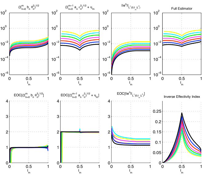
(a) We test duality estimators from Theorem 4.1.

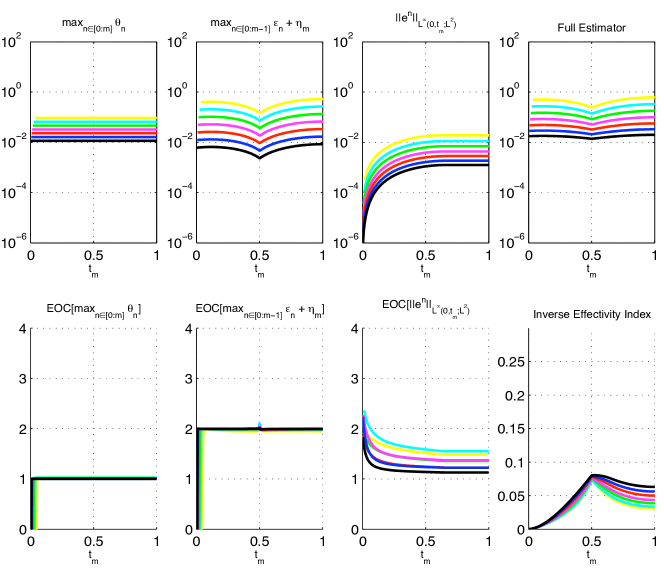
(b) Here we study the estimator from Corollary 4.

Figure 3. Convergence of error and the duality estimators for (7.6) with time-oscillation factor $\kappa=8$ and the other parameters as in Figure 2. We plot all quantities as functions of (PDE) time. Rates for each error/indicator can be read from the experimental order of convergence (EOC) of the associated part of the estimator together with its value on a logarithmic scale. The colour/grey scale is such that dark is finest and light is coarsest. Since the benchmark problem has no initial error, we employ the inverse effectivity index. Note that due to the faster oscillation, how a discrepancy between the error’s time-accumulation (or rather the lack thereof) and the estimator’s builds up quickly and produces oscillations in the effectivity index.

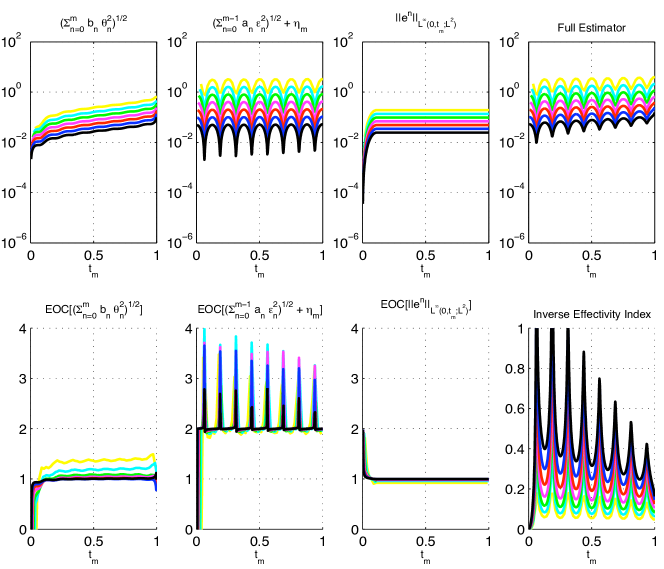
(a) Here we study the estimator from Theorem 4.1.

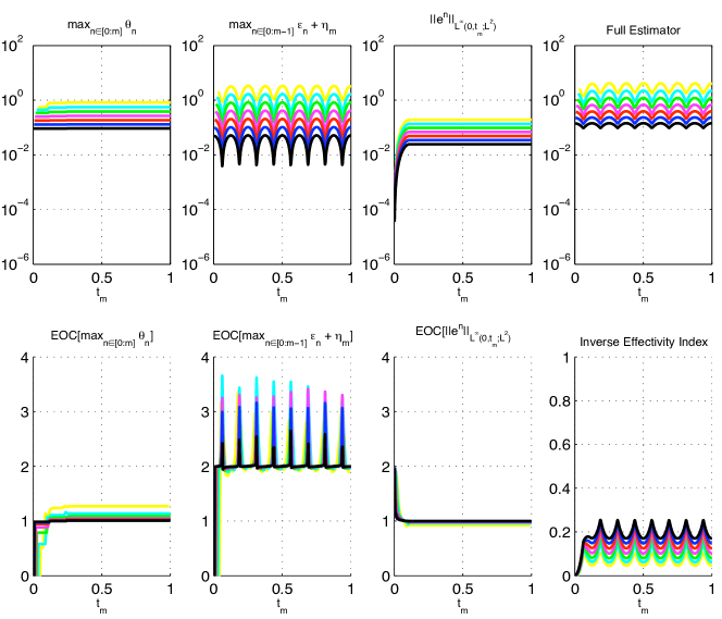
(b) Here we study the estimator from Corollary 4.

Figure 4. Convergence for of the energy-based estimator from Theorem 6.2, taking a uniform timestep $\tau=0.05h$. We couple $\tau$ to appropriate powers of $h$ and with $h(i)=2^{-i}$, $i\in\left[5:11\right]$. In both cases we are using $\mathbb{P}^{1}$ elements. We plot the $\operatorname{EOC}$ of the associated part of the estimator together with its value on a logarithmic scale.

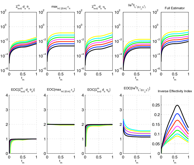
(a) Problem (7.6) with time-oscillation factor $\kappa=1$, to be compared with Figure 2. Convergence rates are clearly similar, but the effectivity index is much more stable (and smooth) with respect to time in this case, as expected given the better accumulation of the estimator in time (cf. Figure 1).

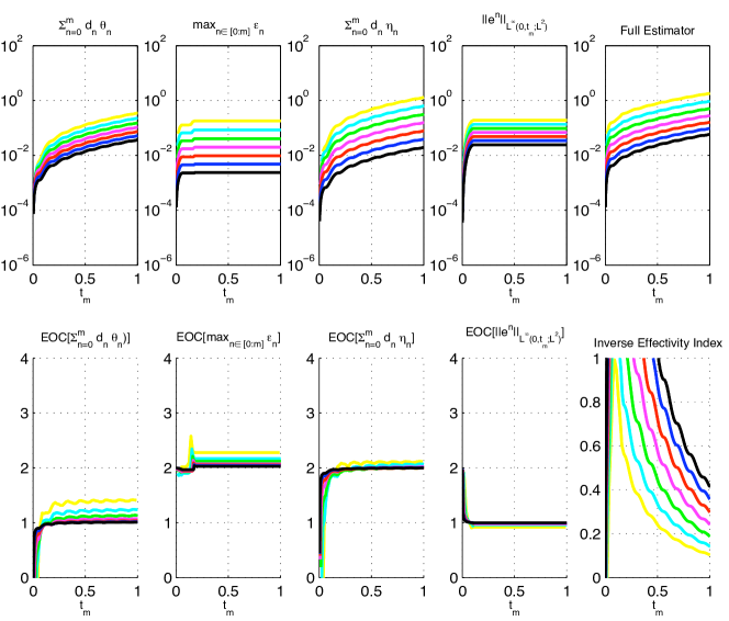
(b) Problem (7.6) with time-oscillation factor $\kappa=8$, to be compared with Figure 3. Here the gain in effectivity index, from using the energy instead of duality estimators is even more dramatic.

References

• Ainsworth and Oden (2000) M. Ainsworth and J. T. Oden. A posteriori error estimation in finite element analysis. Wiley-Interscience [John Wiley & Sons], New York, 2000. ISBN 0-471-29411-X.
• Akrivis et al. (2006) G. Akrivis, C. Makridakis, and R. H. Nochetto. A posteriori error estimates for the Crank-Nicolson method for parabolic equations. Math. Comp., 75(254):511–531 (electronic), 2006. ISSN 0025-5718. doi: 10.1090/S0025-5718-05-01800-4. URL http://dx.doi.org/10.1090/S0025-5718-05-01800-4.
• Bartels and Müller (2009) S. Bartels and R. Müller. Optimal and robust a posteriori error estimates in $l^{\infty}(l^{2})$ for the approximation of allen-cahn equations past singularities. Technical report, Universität Bonn, 2009. URL http://bartels.ins.uni-bonn.de/publications/preprint/BarMul09-pre.pdf.
• Bergam et al. (2005) A. Bergam, C. Bernardi, and Z. Mghazli. A posteriori analysis of the finite element discretization of some parabolic equations. Math. Comp., 74(251):1117–1138 (electronic), 2005. ISSN 0025-5718. doi: 10.1090/S0025-5718-04-01697-7. URL http://dx.doi.org/10.1090/S0025-5718-04-01697-7.
• Bernardi and Verfürth (2004) C. Bernardi and R. Verfürth. A posteriori error analysis of the fully discretized time-dependent Stokes equations. M2AN Math. Model. Numer. Anal., 38(3):437–455, 2004. ISSN 0764-583X. doi: 10.1051/m2an:2004021. URL http://dx.doi.org/10.1051/m2an:2004021.
• Braess (2001) D. Braess. Finite elements. Cambridge University Press, Cambridge, second edition, 2001. ISBN 0-521-01195-7. Theory, fast solvers, and applications in solid mechanics, Translated from the 1992 German edition by Larry L. Schumaker.
• Brenner and Scott (1994) S. C. Brenner and L. R. Scott. The mathematical theory of finite element methods. Springer-Verlag, New York, 1994. ISBN 0-387-94193-2.
• Ciarlet (1978) P. G. Ciarlet. The finite element method for elliptic problems. North-Holland Publishing Co., Amsterdam, 1978. ISBN 0-444-85028-7. Studies in Mathematics and its Applications, Vol. 4.
• de Frutos and Novo (2002) J. de Frutos and J. Novo. Postprocessing the linear finite element method. SIAM J. Numer. Anal., 40(3):805–819 (electronic), 2002. ISSN 0036-1429. doi: 10.1137/S0036142900375438. URL http://dx.doi.org/10.1137/S0036142900375438.
• Demlow and Makridakis (2010) A. Demlow and C. Makridakis. Sharply local pointwise a posteriori error estimates for parabolic problems. Math. Comp., 79(271):1233–1262, March 1 2010. doi: 10.1090/S0025-5718-10-02346-X. URL http://www.ams.org/journals/mcom/2010-79-271/S0025-5718-10-02346-X/home.html.
• Demlow et al. (2009) A. Demlow, O. Lakkis, and C. Makridakis. A posteriori error estimates in the maximum norm for parabolic problems. SIAM Journal on Numerical Analysis, 47(3):2157–2176, 2009. doi: 10.1137/070708792. URL http://arxiv.org/abs/0711.3928.
• Eriksson and Johnson (1991) K. Eriksson and C. Johnson. Adaptive finite element methods for parabolic problems. I. A linear model problem. SIAM J. Numer. Anal., 28(1):43–77, 1991. ISSN 0036-1429. doi: 10.1137/0728003. URL http://dx.doi.org/10.1137/0728003.
• Ern and Meunier (2009) A. Ern and S. Meunier. A posteriori error analysis of Euler–Galerkin approximations to coupled elliptic–parabolic problems. M2AN Math. Model. Numer. Anal., 43(2):353–375, MAR-APR 2009. ISSN 0764-583X. doi: 10.1051/m2an:2008048. URL http://dx.doi.org/10.1051/m2an:2008048.
• Evans (1998) L. C. Evans. Partial differential equations, volume 19 of Graduate Studies in Mathematics. American Mathematical Society, Providence, RI, 1998. ISBN 0-8218-0772-2.
• Georgoulis and Lakkis (2010) E. H. Georgoulis and O. Lakkis. A posteriori error bounds for discontinuous galerkin methods for quasilinear parabolic problems. In P. Hansbo and A. Malqvist, editors, Proceedings of ENUMATH 2009 Uppsala, number preprint available as arXiv.org/1001.2935v1, Berlin, DE., 17 Jan 2010. ENUMATH, Springer-Verlag. URL http://arxiv.org/abs/1001.2935.
• Lakkis and Makridakis (2006) O. Lakkis and C. Makridakis. Elliptic reconstruction and a posteriori error estimates for fully discrete linear parabolic problems. Math. Comp., 75(256):1627–1658 (electronic), October 2006. ISSN 0025-5718. URL http://www.ams.org/mcom/2006-75-256/S0025-5718-06-01858-8/home.html.
• Lakkis and Pryer (2010) O. Lakkis and T. Pryer. Gradient recovery in adaptive finite element methods for parabolic problems. IMA J. Numer. Anal., to appear(galleys):1–35, 2010. URL http://arxiv.org/abs/0905.2764. arXiv:0905.2764.
• Liao and Nochetto (2003) X. Liao and R. H. Nochetto. Local a posteriori error estimates and adaptive control of pollution effects. Numer. Methods Partial Differential Equations, 19(4):421–442, 2003. ISSN 0749-159X. doi: 10.1002/num.10053. URL http://dx.doi.org/10.1002/num.10053.
• Makridakis and Nochetto (2003) C. Makridakis and R. H. Nochetto. Elliptic reconstruction and a posteriori error estimates for parabolic problems. SIAM J. Numer. Anal., 41(4):1585–1594 (electronic), 2003. ISSN 1095-7170.
• Picasso (1998) M. Picasso. Adaptive finite elements for a linear parabolic problem. Comput. Methods Appl. Mech. Engrg., 167(3-4):223–237, 1998. ISSN 0045-7825. doi: 10.1016/S0045-7825(98)00121-2. URL http://dx.doi.org/10.1016/S0045-7825(98)00121-2.
• Schmidt and Siebert (2005) A. Schmidt and K. G. Siebert. Design of adaptive finite element software, volume 42 of Lecture Notes in Computational Science and Engineering. Springer-Verlag, Berlin, 2005. ISBN 3-540-22842-X. URL http://www.alberta-fem.de. The finite element toolbox ALBERTA, With 1 CD-ROM (Unix/Linux).
• Thomée (2006) V. Thomée. Galerkin finite element methods for parabolic problems, volume 25 of Springer Series in Computational Mathematics. Springer-Verlag, Berlin, second edition, 2006. ISBN 978-3-540-33121-6; 3-540-33121-2.
• Verfürth (1996) R. Verfürth. A review of a posteriori error estimation and adaptive mesh-refinement techniques. Wiley-Teubner, Chichester-Stuttgart, 1996. ISBN 0-471-96795-5.