On a Class of Metrics Related to
Graph Layout Problems

Abstract.

We examine the metrics that arise when a finite set of points is embedded in the real line, in such a way that the distance between each pair of points is at least $1$. These metrics are closely related to some other known metrics in the literature, and also to a class of combinatorial optimization problems known as graph layout problems. We prove several results about the structure of these metrics. In particular, it is shown that their convex hull is not closed in general. We then show that certain linear inequalities define facets of the closure of the convex hull. Finally, we characterise the unbounded edges of the convex hull and of its closure.
Key Words: metric spaces, graph layout problems, convex analysis, polyhedral combinatorics.

1. Introduction

For a given positive integer $n$, let $[n]$ denote $\{1,\dots,n\}$. A metric on $[n]$ is a mapping $d\colon[n]\times[n]\to\mathbb{R}_{+}$ which satisfies the following three conditions:

• $d(i,j)=d(j,i)$ for all $\{i,j\}\subset[n]$,

• $d(i,k)+d(j,k)\geq d(i,j)$ for all ordered triples $(i,j,k)\subset[n]$,

• $d(i,j)=0$ if and only if $i=j$.

Metrics are a special case of semimetrics, which are obtained by dropping ‘and only if’ from the third condition. There is a huge literature on metrics and semimetrics; see for example [12]. The inequalities in the second condition are the well-known triangle inequalities.

In this paper we study the metrics $d$ on $[n]$ that arise when $n$ points are embedded in the real line, in such a way that the distance between each pair of points is at least $1$. More formally, we require that $d$ satisfies the following two properties:

• there exist real numbers $r_{1},\dots,r_{n}$ such that $d(i,j)={\left\lvert{r_{i}-r_{j}}\right\rvert}$ for all $\{i,j\}\subset[n]$;

• $d(i,j)\geq 1$ for all $\{i,j\}\subset[n]$.

We remark that one could easily replace the value $1$ with some arbitrary constant $\epsilon>0$; the results in this paper would remain essentially unchanged.

We call the metrics in question ‘$\mathbb{R}$-embeddable $1$-separated’ metrics. We believe that these metrics are a natural object of study, and of interest in their own right. We have, however, two specific motives for studying them. First, they are closely related to certain well-known metrics that have appeared in the literature. Second, they are also closely related to an important class of combinatorial optimization problems, known as graph layout problems.

As well as studying the metrics themselves, we also study their convex hull. It turns out that the convex hull is not always closed, which leads us to study also the closure of the convex hull. Among other things, we characterise some of the $(n-1)$-dimensional faces (i. e., facets) of the closure, and some of the $1$-dimensional faces (i. e., edges) of both the convex hull and its closure.

The structure of the paper is as follows. In Section 2, we review some of the relevant literature on metrics and graph layout problems. In Section 3, we present various results concerned with the structure of the metrics and their convex hull. Next, in Section 4, we present some inequalities that define facets of the closure of the convex hull. In Section 5, we give a combinatorial characterisation of the unbounded edges of the convex hull and of its closure. Finally, some concluding remarks are given in Section 6.

We close this section with a word on notation. To study convex geometric properties, we view metrics as points in a vector space ${\mathbb{S}}\mspace{-3.2mu}{}^{\scriptscriptstyle 0}_{n}$. In our notation, ${\mathbb{S}}\mspace{-3.2mu}{}^{\scriptscriptstyle 0}_{n}$ will be either the vector space of all symmetric functions $[n]\times[n]\to\mathbb{R}$ or the vector space of all real symmetric $(n\times n)$-matrices whose diagonal entries are zero, and we will switch freely between them. For the latter, the inner product is defined as usual by

$$A\bullet B:=\operatorname{tr}(A^{\mspace{-1.0mu}\scriptscriptstyle\top\mspace{-1.0mu}}B)=\sum_{k=1}^{n}\sum_{l=1}^{n}A_{k,l}B_{k,l}.$$

We understand a metric both as a function and a matrix, and we will switch between the two concepts without further mentioning.

By $S(n)$ we denote the set of all permutations of $[n]$. We occasionally view $S(n)$ as a subset of $\mathbb{R}^{d}$ by identifying the permutation $\pi$ with the point $(\pi(1),\dots,\pi(n))^{\mspace{-1.0mu}\scriptscriptstyle\top\mspace{-1.0mu}}$. Furthermore we let $\imath_{n}:=(1,\dots,n)$ the identity permutation in $S(n)$. We omit the index $n$ when no confusion can arise. $\mathbf{1}$ is a column vector of appropriate length consisting of ones. Similarly $\mathbf{0}$ is a vector whose entries are all zero. If appropriate, we will use a subscript $\mathbf{1}_{k}$, $\mathbf{0}_{k}$ to identify the length of the vectors. The symbol $\operatorname{\mathbb{0}}0$ denotes an all-zeros matrix not necessarily square, and we also use it to say “this part of the matrix consists of zeros only.” By ${{\mathbb{1}}_{n}}$ we denote the square matrix of order $n$ whose $(k,l)$-entry is $1$ if $k\neq l$ and $0$ otherwise. As above we will omit the index $n$ when appropriate. We denote by $\complement U$ the complement of the set $U$.

2. Literature Review

In this section, we review some of the relevant literature. We cover related semimetrics in Subsection 2.1 and graph layout problems in Subsection 2.2. To facilitate reading we have summarized all matrix sets discussed in Table 1.

CUTn	$\ell_{1}$-embeddable semimetrics (cut cone)
HYPn	hypermetrics, see (1)
NEGn	negative-type cone, see (2)
$M_{n}^{L2}$	$\ell_{2}$-embeddable semimetrics
$M_{n}^{R}$	$\mathbb{R}$-embeddable semimetrics
$M_{n}^{R1}$	$\mathbb{R}$-embeddable $1$-separated metrics
$Q_{n}$	convex hull of $M_{n}^{R1}$
$\overline{Q_{n}}$	closure of $Q_{n}$
$P_{n}$	permutation metrics polytope, see (5)

Table 1. Sets of matrices

2.1. Some related semimetrics

The following four classes of semimetrics on $[n]$, which are closely related to the $\mathbb{R}$-embeddable $1$-separated metrics, have been extensively studied in the literature (see [12] for a detailed survey):

• The $\ell_{1}$-embeddable semimetrics, i. e., those for which there exist a positive integer $m$ and points $x_{1},\dots,x_{n}\in\mathbb{R}^{m}$ such that $d(i,j)={\left\lvert{x_{i}-x_{j}}\right\rvert_{1}}:=\sum_{k=1}^{m}{\left\lvert{x_{ik}-x_{jk}}\right\rvert}$ for all $\{i,j\}\subset[n]$.

• The $\ell_{2}$-embeddable semimetrics, which are defined as in the $\ell_{1}$ case, except that $d(i,j)={\left\lvert{x_{i}-x_{j}}\right\rvert_{2}}:=\sqrt{\sum_{k=1}^{m}(x_{ik}-x_{jk})^{2}}$.

• The $\mathbb{R}$-embeddable semimetrics, which are the special case of $\ell_{1}$- (or $\ell_{2}$-) embeddable semimetrics obtained when $m=1$.

• The hypermetrics, which are semimetrics that satisfy the following hypermetric inequalities [10]:

  (1) $$\sum_{\{i,j\}\subset[n]}b_{i}b_{j}d(i,j)\leq 0\qquad(\forall b\in\mathbb{Z}^{n}:\sum_{i=1}^{n}b_{i}=1).$$

It is known [4] that the set of $\ell_{1}$-embeddable semimetrics on $[n]$ is a polyhedral cone in $\mathbb{R}^{\binom{n}{2}}$. In fact, it is nothing but the well-known cut cone, denoted by CUT_n. The set of all hypermetrics on $[n]$, called the hypermetric cone and denoted by HYP_n, is also polyhedral [11].

We will let $M_{n}^{L2}$ and $M_{n}^{R}$ denote the set of $\ell_{2}$- and $\mathbb{R}$-embeddable semimetrics, respectively. It is known that $M_{n}^{L2}$ and $M_{n}^{R}$ are not convex (unless $n$ is small), and that the convex hull of $M_{n}^{L2}$ and $M_{n}^{R}$ is CUT_n. It is also known [21] that a symmetric function $d$ lies in $M_{n}^{L2}$ if and only if $d^{2}$ (i. e., the symmetric function obtained by squaring each value) lies in the so-called negative-type cone. The negative-type cone, denoted by NEG_n, is the (non-polyhedral) cone defined by the following negative-type inequalities:

(2) $$\sum_{\{i,j\}\subset[n]}b_{i}b_{j}d(i,j)\leq 0\qquad(\forall b\in\mathbb{R}^{n}:\sum_{i=1}^{n}b_{i}=0).$$

The structure of $M_{n}^{R}$ and related sets is studied in [5].

In recent years, there has been a stream of papers on so-called negative-type semimetrics (also known as $\ell_{2}^{2}$-semimetrics) [2, 3, 9, 16, 17, 18]. These are simply semimetrics that lie in NEG_n. They have been used to derive approximation algorithms for various combinatorial optimisation problems, including the graph layout problems that we mention in the next subsection.

The following inclusions are known: $M_{n}^{R}\subset M_{n}^{L2}\subset$ CUT${}_{n}\subset$ HYP${}_{n}\subset$ NEG_n. Denoting the set of all $\mathbb{R}$-embeddable $1$-separated metrics by $M_{n}^{R1}$, we obtain from their definition $M_{n}^{R1}\subset M_{n}^{R}$. We will explore the relationship between $M_{n}^{R1}$, $M_{n}^{R}$ and CUT_n further in Subsection 3.1.

2.2. Graph layout problems

Given a graph $G=(V,E)$, with $V=[n]$, a layout is simply a permutation of $[n]$. If we view a layout $\pi\in S(n)$ as a placing of the vertices on points $1,\ldots,n$ along the real line, the quantity $|\pi(i)-\pi(j)|$ corresponds to the Euclidean distance between vertices $i$ and $j$. Several important combinatorial optimization problems, collectively known as graph layout problems, call for a layout minimising a function of these distances (see the survey [13]). For example, in the Minimum Linear Arrangement Problem (MinLA), the objective is to minimize $\sum_{\{i,j\}\in E}|\pi(i)-\pi(j)|$. In the Bandwidth Problem, the objective is to minimise $\max_{\{i,j\}\in E}|\pi(i)-\pi(j)|$.

Now, let $d(i,j)$ for $\{i,j\}\subset[n]$ be a decision variable, representing the quantity $|\pi(i)-\pi(j)|$. It has been observed by several authors that interesting relaxations of graph layout problems can be formed by deriving valid linear inequalities that are satisfied by all feasible symmetric functions $d$. To our knowledge, the first paper of this kind was [19], which presented the following star inequalities:

(3) $$\sum_{j\in S}d(i,j)\geq\lfloor({\left\lvert{S}\right\rvert}+1)^{2}/4\rfloor.$$

Here, $i\in[n]$ and $S\subset[n]\setminus\{i\}$ is such that every node in $S$ is adjacent to $i$.

Apparently independently, Even et al. [14] defined the so-called spreading metrics. These are metrics that satisfy the following spreading inequalities:

(4) $$\sum_{j\in S}d(i,j)\geq{\left\lvert{S}\right\rvert}({\left\lvert{S}\right\rvert}+2)/4\qquad(\forall i\in[n],\forall S\subseteq[n]\setminus\{i\}).$$

Note that the spreading inequalities are more general than the star inequalities, but have a slightly weaker right-hand side when $n$ is odd. Spreading metrics were used in [14, 20] to derive approximation algorithms for various graph layout problems.

In [8, 15], it was noted that one can get a tighter relaxation of graph layout problems by requiring the spreading metrics to lie in the negative-type cone NEG_n. The authors called the resulting metrics $\ell_{2}^{2}$-spreading metrics.

A natural way to derive further valid linear inequalities for graph layout problems is to study the following permutation metrics polytope:

(5) $$P_{n}=\operatorname{conv}\Bigl{\{}d\Bigm{|}\exists\pi\in S(n):\;d(i,j)={\left\lvert{\pi(i)-\pi(j)}\right\rvert}\;\forall\{i,j\}\subset[n]\Bigr{\}}.$$

Surprisingly, this was not done until very recently [1]. In [1], it is shown that $P_{n}$ is of dimension $\binom{n}{2}-1$ and that its affine hull is defined by the equation $\sum_{\{i,j\}\subset[n]}d(i,j)=\binom{n+1}{3}$. It is also shown that the following four classes of inequalities define facets of $P_{n}$ under mild conditions:

• pure hypermetric inequalities, which are simply the hypermetric inequalities (1) for which $b\in\{0,\pm 1\}^{n}$;

• strengthened pure negative-type inequalities, which are like the negative-type inequalities (2) for which $b\in\{0,\pm 1\}^{n}$, except that the right-hand side is increased from $0$ to $\frac{1}{2}\sum_{i\in[n]}|b_{i}|$;

• clique inequalities, which take the form

  (6) $$\sum_{\{i,j\}\subset S}d(i,j)\geq\binom{|S|+1}{3},$$

  where $S\subset[n]$ satisfies $2\leq|S|<n$;

• strengthened star inequalities, which take the form

  (7) $$(|S|-1)\sum_{i\in S}d(r,i)-\sum_{\{i,j\}\subset S}d(i,j)\geq\left\lfloor(|S|+1)^{2}(|S|-1)/12\right\rfloor,$$

  where $r\in V$ and $S\subseteq V\setminus\{r\}$ with $|S|\geq 2$.

It is pointed out in the same paper that each star inequality (3) with $|S|\geq 2$ is dominated by a clique inequality (6) and a strengthened star inequality (7). Therefore, very few of the star inequalities define facets of $P_{n}$.

Finally, we mention that some more valid inequalities were presented recently by Caprara et al. [7]. Some of them were proved to define facets of the dominant of $P_{n}$, though not of $P_{n}$ itself.

We will establish an interesting connection between $M_{n}^{R1}$, CUT_n and $P_{n}$ in Subsection 3.2.

3. On $M_{n}^{R1}$ and its Convex Hull

3.1. On $M_{n}^{R1}$ and related sets

We now study $M_{n}^{R1}$ and its relationship with $M_{n}^{R}$, $P_{n}$ and CUT_n. We will find it helpful to recall the definition of a cut metric:

Definition 3.1.

For a set $U\subset[n]$, we let $d_{U}$ be the metric which assigns to two points on different sides of the bipartition $U,\complement U$ of $[n]$ a value of $1$ and to points on the same side a value of $0$.

We will say that the set $U$ induces the associated cut metric. In other words, if we let $D_{k,l}(x):={\left\lvert{x_{k}-x_{l}}\right\rvert}$ for every vector $x\in\mathbb{R}^{n}$ (and identify, as promised, functions and matrices), then $d_{U}=D(\chi^{U})$. With this notation, CUT_n is the convex cone with apex $0$ in ${\mathbb{S}}\mspace{-3.2mu}{}^{\scriptscriptstyle 0}_{n}$ generated by the points $d_{U}$, i. e.,

$$\text{CUT}_{n}:=\operatorname{cone}\Bigl{\{}d_{U}\Bigm{|}d_{U}\;\text{is the cut metric for}\;U\subset[n]\Bigr{\}}.$$

It is known [6] that each cut metric defines an extreme ray of CUT_n.

We will also need the following notation. For a given permutation $\pi\in S(n)$, let $N_{\pi}$ be the set of $x\in\mathbb{R}^{n}$ which satisfy $x_{\pi(i)}\leq x_{\pi(i+1)}$ for $i=1,\ldots,n-1$. Now let $M(\pi)$ denote the set of metrics $d$ for which there exists an $x\in N_{\pi}$ with $d=D(x)$. Also, for a given $\pi$ and for $k=1,\ldots,n-1$, we emphasize that $D(\chi^{\pi^{-1}([k])})$ is the cut metric induced by the set $U=\{\pi^{-1}(1),\ldots,\pi^{-1}(k)\}$. (So, for example, if $n=4$ and $\pi=\{2,3,1,4\}$, then $D(\chi^{\pi^{-1}([2])})$ is the cut metric induced by the set $\{2,3\}$.)

We have the following lemma:

Lemma 3.2.

$M(\pi)$ is a polyhedral cone of dimension $n-1$ defined by the $n-1$ cut metrics $D(\chi^{\pi^{-1}([1]))},\ldots,D(\chi^{\pi^{-1}([n-1])})$.

Proof.

Let $d^{*}\in M(\pi)$ and let $x_{1},\ldots,x_{n}$ be the corresponding points in $\mathbb{R}$. One can check that:

$$d^{*}=\sum_{k=1}^{n-1}(x_{k+1}-x_{k})D(\chi^{\pi^{-1}([k])}).$$

From the definition of $M(\pi)$, we have $x_{k+1}-x_{k}\geq 0$ for $k=1,\ldots,n-1$. Thus, $d^{*}$ is a conical combination of the $n-1$ cut metrics mentioned. This shows that $M(\pi)$ is contained in the cone mentioned. The reverse direction is similar. ∎

This enables us to describe the structure of $M_{n}^{R}$:

Proposition 3.3.

$M_{n}^{R}$ is the union of $n!/2$ polyhedral cones, each of dimension $n-1$.

We define the antipodal permutation of $\pi\in S(n)$ by

$$\pi^{-}:=(n+1)\cdot\mathbf{1}-\pi.$$

This is the permutation obtained by reversing $\pi$. A swift computation shows that $D(\pi)=D(\pi^{-})$.

Proof.

From the definitions, we have $M_{n}^{R}=\bigcup_{\pi\in S(n)}M(\pi)$. From the above lemma, the set $M(\pi)$ is a polyhedral cone of dimension $n-1$. Now, note that, for any $\pi\in S(n)$, we have $M(\pi)=M(\pi^{-})$. Thus, the union can be taken over $n!/2$ permutations, instead of over all permutations. ∎

We note in passing that every cut metric belongs to $M(\pi)$ for some $\pi\in S(n)$. This explains the well-known fact, mentioned in Subsection 2.1, that the convex hull of $M_{n}^{R}$ is equal to CUT_n.

Now, we adapt these results to the case of $M_{n}^{R1}$. We define $M^{1}(\pi)$ similar to $M(\pi)$: we denote by $M^{1}(\pi)$ the set of all metrics $d$ which are of the form $D(x)$ for an $x\in\mathbb{R}^{n}$ which satisfies $x_{\pi(i)}+1\leq x_{\pi(i+1)}$ for $i=1,\ldots,n-1$.

Note that the $D(\pi)$ are nothing but the metrics associated with feasible layouts, which by a result in [1] are the extreme points of $P_{n}$. Note also that the sets $M^{1}(\pi)$ are disjoint.

We have the following lemma:

Lemma 3.4.

$M^{1}(\pi)$ is the Minkowski sum of the point $D(\pi)$ and the cone $M(\pi)$:

$$M^{1}(\pi)=D(\pi)+D(N_{\pi}).$$

Proof.

This can be proven in the same way as Lemma 3.2. The only difference is that we decompose $d^{*}\in M^{1}(\pi)$ as:

$$d^{*}=D(\pi)+\sum_{k=1}^{n-1}(r_{k+1}-r_{k}-1)D(\chi^{\pi^{-1}([k])}),$$

and note that $r_{k+1}-r_{k}-1\geq 0$ for $k=1,\ldots,n-1$. ∎

We can now derive an analog of Proposition 3.3:

Proposition 3.5.

$M_{n}^{R1}$ is the union of $n!/2$ disjoint translated polyhedral cones, each of dimension $n-1$.

Proof.

From the definitions, we have $M_{n}^{R1}=\bigcup_{\pi\in S(n)}M^{1}(\pi)$. From Lemmas 3.2 and 3.4, each set $M^{1}(\pi)$ is a translated polyhedral cone of dimension $n-1$. As in the proof of Proposition 3.3, the union can be taken over only $n!/2$ permutations. ∎

3.2. On the convex hull of $M_{n}^{R1}$ and related sets

We now turn our attention to the convex hull of $M_{n}^{R1}$, which we denote by $Q_{n}$. To give some intuition, we present in Fig. 1 drawings of $M_{n}^{R1}$ and $Q_{3}$ from three different angles. (Of course, the drawing is truncated, since $Q_{3}$ is unbounded.) The three co-ordinates represent $d(1,2)$, $d(1,3)$ and $d(2,3)$. The three coloured regions represent the three disjoint subsets of $M_{3}^{R1}$ mentioned in Proposition 3.5.

One can see that $Q_{3}$ is a three-dimensional polyhedron, with one bounded facet, six unbounded facets, three bounded edges and six unbounded edges.

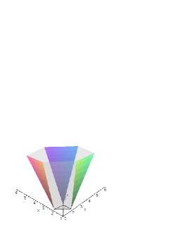
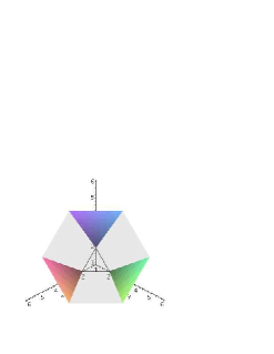
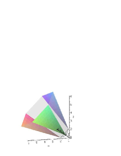
Figure 1. The convex set $Q_{3}$

For $n\leq 3$, $Q_{n}$ is closed (and therefore a polyhedron). We will show in Section 5, however, that $Q_{n}$ is not closed for $n\geq 4$. Therefore, we are led to look at the closure of $Q_{n}$, which we denote by $\overline{Q_{n}}$.

Our next result shows that there is a close connection between the polyhedron $\overline{Q_{n}}$, the polytope $P_{n}$, and the cone CUT_n:

Proposition 3.6.

$\overline{Q_{n}}$ is the Minkowski sum of $P_{n}$ and CUT_n.

Proof.

We use the same notation as in the previous subsection. By definition, every point in $M_{n}^{R1}$ belongs to $M^{1}(\pi)$ for some $\pi\in S(n)$. From Lemma 3.4, every point in $M^{1}(\pi)$ is the sum of the point $D(\pi)$ and a point in the cut cone CUT_n. Moreover, the point $D(\pi)$ is an extreme point of $P_{n}$. Thus, every point in $M_{n}^{R1}$ is the sum of an extreme point of $P_{n}$ and a point in CUT_n. Since $\overline{Q_{n}}$ is the closure of the convex hull of $M_{n}^{R1}$, it must be contained in the Minkowski sum of $P_{n}$ and CUT_n. The reverse direction is proved similarly, noting that every cut metric is of the form $D(\chi^{\pi^{-1}([k])})$ for some $\pi\in S(n)$ and some $k\in[n-1]$. ∎

This immediately implies the following result:

Corollary 3.7.

$\overline{Q_{n}}$ is full-dimensional (i. e., of dimension $\binom{n}{2}$).

We also have the following result:

Proposition 3.8.

$P_{n}$ is the unique bounded facet of $\overline{Q_{n}}$.

Proof.

As mentioned in the previous section, all points in $P_{n}$ satisfy the equation $\sum_{\{i,j\}\subset[n]}d(i,j)=\binom{n+1}{3}$. Moreover, every point in CUT_n satisfies $\sum_{\{i,j\}\subset[n]}d(i,j)>0$. Since $\overline{Q_{n}}$ is the Minkowski sum of $P_{n}$ and CUT_n, it follows that the inequality $\sum_{\{i,j\}\subset[n]}d(i,j)\geq\binom{n+1}{3}$ is valid for $\overline{Q_{n}}$ and that $P_{n}$ is the face of $\overline{Q_{n}}$ exposed by this inequality. Since $\overline{Q_{n}}$ and $P_{n}$ are of dimension $\binom{n}{2}$ and $\binom{n}{2}-1$, respectively, $P_{n}$ is a facet of $\overline{Q_{n}}$. It must be the unique bounded facet, since all extreme points of $\overline{Q_{n}}$ are in $P_{n}$. ∎

In the next section, we will explore the connection between $\overline{Q_{n}}$, $P_{n}$ and CUT_n in more detail. To close this section, we make an observation about how the individual ‘pieces’ of $M_{n}^{R1}$, called the $M^{1}(\pi)$ in the previous subsection, are positioned within $\overline{Q_{n}}$:

Proposition 3.9.

For any $\pi\in S(n)$, the set $M^{1}(\pi)$ is an $(n-1)$-dimensional face of $\overline{Q_{n}}$.

Proof.

By definition, $\overline{Q_{n}}$ satisfies all triangle inequalities. Now, without loss of generality, suppose that $\pi$ is the identity permutation. Every point in $M^{1}(\pi)$ satisfies all of the following triangle inequalities at equality:

$$d(i,j)+d(j,k)\geq d(i,k)\qquad(\forall 1\leq i<j<k\leq n).$$

Moreover, no other point in $M_{n}^{R1}$ does so. Thus, $M^{1}(\pi)$ is a face of $\overline{Q_{n}}$. It was shown to be $(n-1)$-dimensional in the previous subsection. ∎

4. Inequalities Defining Facets of $\overline{Q_{n}}$

In this section, we study linear inequalities that define facets of $\overline{Q_{n}}$, i. e., faces of dimension $\binom{n}{2}-1$. Subsection 4.1 presents some general results about such inequalities, whereas Subsection 4.2 lists some specific inequalities.

4.1. General results on facet-defining inequalities

In this subsection, we prove a structural result about inequalities that define facets of $\overline{Q_{n}}$, and show how this can be used to construct facets of $\overline{Q_{n}}$ in a mechanical way from facets of either $P_{n}$ or CUT_n.

We will need the following definition, taken from [1]:

Definition 4.1 (Amaral & Letchford, 2009).

Let $\alpha^{T}d\geq\beta$ be a linear inequality, where $\alpha,d\in\mathbb{R}^{\binom{n}{2}}$. The inequality is said to be ‘canonical’ if:

(8) $$\min_{\emptyset\neq S\subset[n]}\sum_{i\in S}\sum_{[n]\setminus S}\alpha_{ij}=0.$$

By definition, an inequality $\alpha^{T}d\geq 0$ defines a proper face of CUT_n if and only if it is canonical. In [1], it is shown that every facet of $P_{n}$ is defined by a canonical inequality. The following lemma is the analogous result for $\overline{Q_{n}}$:

Lemma 4.2.

Every unbounded facet of $\overline{Q_{n}}$ is defined by a canonical inequality.

Proof.

Suppose that the inequality $\alpha^{T}d\geq\beta$ defines an unbounded facet of $\overline{Q_{n}}$. Since $\overline{Q_{n}}$ is the Minkowski sum of $P_{n}$ and CUT_n, the inequality must be valid for CUT_n. Therefore, the left-hand side of (8) must be non-negative. Moreover, since the inequality defines an unbounded facet, there must be at least one extreme ray of CUT_n satisfying $\alpha^{T}d=0$. Therefore the left-hand side of (8) cannot be positive. ∎

We remind the reader that only one facet of $\overline{Q_{n}}$ is bounded (Proposition 3.8).

Now, we show how to derive facets of $\overline{Q_{n}}$ from facets of $P_{n}$:

Proposition 4.3.

Let $F$ be any facet of $P_{n}$, and let $\alpha^{T}d\geq\beta$ be the canonical inequality that defines it. This inequality defines a facet of $\overline{Q_{n}}$ as well.

Proof.

The fact that the inequality is valid for $\overline{Q_{n}}$ follows from the fact that $\overline{Q_{n}}$ is the Minkowski sum of $P_{n}$ and CUT_n. Now, since $F$ is a facet of $P_{n}$, there exist $\binom{n}{2}-1$ affinely-independent vertices of $P_{n}$ that satisfy the inequality at equality. Moreover, since the inequality is canonical, there exists at least one extreme ray of CUT_n that satisfies $\alpha^{T}d=0$. Since $\overline{Q_{n}}$ is the Minkowski sum of $P_{n}$ and CUT_n, there exist $\binom{n}{2}$ affinely-independent points in $\overline{Q_{n}}$ that satisfy the inequality at equality. Thus, the inequality defines a facet of $\overline{Q_{n}}$. ∎

Now, we show how to derive facets of $\overline{Q_{n}}$ from facets of CUT_n:

Proposition 4.4.

Let $\alpha^{T}d\geq 0$ define a facet of CUT_n, and let $\beta$ be the minimum of $\alpha^{T}d$ over all $d\in P_{n}$. Then the inequality $\alpha^{T}d\geq\beta$ define a facet of $\overline{Q_{n}}$.

Proof.

As before, the fact that the inequality $\alpha^{T}d\geq\beta$ is valid for $\overline{Q_{n}}$ follows from the fact that $\overline{Q_{n}}$ is the Minkowski sum of $P_{n}$ and CUT_n. Now, since the inequality $\alpha^{T}d\geq 0$ defines a facet of CUT_n, there exist $\binom{n}{2}-1$ linearly-independent extreme rays of CUT_n that satisfy $\alpha^{T}d=0$. Moreover, from the definition of $\beta$, there exists at least one extreme point of $P_{n}$ that satisfies $\alpha^{T}d=\beta$. Since $\overline{Q_{n}}$ is the Minkowski sum of $P_{n}$ and CUT_n, there exist $\binom{n}{2}$ affinely-independent points in $\overline{Q_{n}}$ that satisfy $\alpha^{T}d=\beta$. Thus, the inequality $\alpha^{T}d\geq\beta$ defines a facet of $\overline{Q_{n}}$. ∎

4.2. Some specific facet-defining inequalities

The results in the previous subsection enable one to derive a wide variety of facets of $\overline{Q_{n}}$. In this subsection, we briefly examine some specific valid inequalities; namely, the inequalities mentioned in [1].

First, we deal with the clique and pure hypermetric inequalities:

Proposition 4.5.

The clique inequalities (6) define facets of $\overline{Q_{n}}$ for all $S\subseteq[n]$ with $|S|\geq 2$.

Proof.

It was shown in [1] that the clique inequalities define facets of $P_{n}$ when $S$ is a proper subset of $[n]$. In this case, the inequalities are canonical and so, by Proposition 4.3, they define facets of $\overline{Q_{n}}$ as well. The case $S=[n]$ is covered in the proof of Proposition 3.8. ∎

Proposition 4.6.

All pure hypermetric inequalities define facets of $\overline{Q_{n}}$.

Proof.

It was shown in [6] that all pure hypermetric inequalities define facets of CUT_n. It was also shown in [1] that every pure hypermetric inequality is satisfed at equality by at least one extreme point of $P_{n}$. The result then follows from Proposition 4.4. ∎

As for the strengthened pure negative-type and strengthened star inequalities, it was shown in [1] that they define facets of $P_{n}$ under certain conditions. Since they are canonical, they define facets of $\overline{Q_{n}}$ under the same conditions. In fact, using the same proof technique used in [1], one can show the following two results:

Proposition 4.7.

All strengthened pure negative-type inequalities define facets of $\overline{Q_{n}}$.

Proposition 4.8.

Strengthened star inequalities define facets of $\overline{Q_{n}}$ if and only if $|S|\neq 4$.

We omit the proofs, for the sake of brevity.

5. Unbounded Edges of $Q_{n}$ and $\overline{Q_{n}}$

5.1. Unbounded edges of $Q_{n}$

We now investigate how the polyhedral cones $M^{1}(\pi)=D(\pi)+D(N_{\pi})$ as subsets of $Q_{n}$. In Fig. 1, it can be seen that in the case $n=3$, the three cones are faces of $Q_{3}$ (recall that $Q_{3}$ is a polyhedron, which means that we can safely speak of faces). In the following proposition, we show that this is the case for all $n$, and we also characterize the extremal half-lines of $Q_{n}$. This will be useful in comparing $Q_{n}$ with its closure: We will characterize the unbounded edges issuing from each vertex for the polyhedron $\overline{Q_{n}}=P_{n}+$CUT_n in the following subsection.

We are dealing with an unbounded convex set of which we do not know whether it is closed or not. (In fact, we will show that $Q_{n}$ is almost never closed). For this purpose, we supply the following fact for easy reference.

Fact 5.1.

For $k=1,\dots,m$ let $K_{k}$ be a (closed) polyhedral cone with apex $x_{k}$. Suppose that the $K_{k}$ are pairwise disjoint and define $S:=\biguplus_{k=1}^{m}K_{k}$. Let $x,y$ be vectors such that $x+\mathbb{R}_{+}y$ is an extremal subset of $\operatorname{conv}(S)$. It then follows that there exists a $\lambda_{0}\in\mathbb{R}_{+}$ and a $k$ such that $x+\lambda y\in K_{k}$ for all $\lambda\geq\lambda_{0}$. Since $x+\mathbb{R}_{+}y$ is extremal, this implies that there exists a $\lambda_{1}\in\mathbb{R}_{+}$ such that $x_{k}=x+\lambda_{1}y$ and $x_{k}+\mathbb{R}_{+}y=\{x+\lambda y\mid\lambda\geq\lambda_{1}\}$ is an extreme ray of the polyhedral cone $K_{k}$.

Definition 5.2.

We say that a permutation $\pi$ and a non-empty set $U\subsetneq[n]$ are incident, if $U=\{\pi^{-1}(1),\dots,\pi^{-1}(k)\}$, where $k:={\left\lvert{U}\right\rvert}$.

Proposition 5.3.

1. For every $\pi\in S(n)$, each edge of the cone $D(\pi)+D(N_{\pi})$ is an exposed subset of $Q_{n}$.

2. The unbounded one dimensional extremal sets of $Q_{n}$ are exactly the defining half-lines. In other words, every half-line $X+\mathbb{R}_{+}Y$ which is an extremal subset of $Q_{n}$ is of the form $D(\pi)+\mathbb{R}_{+}D(\chi^{U})$ for a $\pi\in S(n)$ and a set $U$ incident to $\pi$. In particular, for every vertex $D(\pi)$ of $Q_{n}$, the unbounded one-dimensional extremal subsets of $Q_{n}$ containing $D(\pi)$ are in bijection with the non-empty proper subsets of $[n]$ incident to $\pi$. Thus there are precisely $n-1$ of them.

Proof.

i. By symmetry it is sufficient to treat the case $\pi=\imath:=(1,\dots,n)^{\mspace{-1.0mu}\scriptscriptstyle\top\mspace{-1.0mu}}$, the identity permutation. Consider the matrix

$$C:={\left(\begin{smallmatrix}0&1&&&&&-1\\ 1&0&1&&&\operatorname{\mathbb{0}}0&\\ ~{}&1&&&&&\\ ~{}&&&\ddots&&&\\ ~{}&&&&&1&\\ ~{}&\operatorname{\mathbb{0}}0&&&1&0&1\\ -1&&&&&1&0\end{smallmatrix}\right)}\in{\mathbb{S}}\mspace{-3.2mu}{}^{\scriptscriptstyle 0}_{n}.$$

It is easy to see that the minimum over all $C\bullet D(\pi)$, $\pi\in S(n)$, is attained only in $\pi=\imath,\imath^{-}$ with the value $0$. Moreover, for any non-empty proper subset $U$ of $[n]$, we have $C\bullet D(\chi^{U})=0$ if $U$ is incident to $\imath$ and $C\bullet D(\chi^{U})>0$ otherwise. Hence, we have that $D(\imath)+D(N_{\imath})$ is equal to the set of all points in $Q_{n}$ which satisfy the valid inequality $C\bullet X\geq 0$ with equality. Out of this matrix $C$ we will now construct a matrix $C^{\prime}$ and a right hand side such that only some of the subsets incident to $\imath$ fulfill the inequality with equality. To do so let $U_{0}$ be a subsets of $[n]$ incident to $\imath$. If, for each $U\subset[n]$ incident to $\imath$ but different from $U_{0}$, we increase the matrix entries $C_{\max U,\max U+1}$ and $C_{\max U+1,\max U}$ by one, we obtain an inequality $C^{\prime}\bullet X\geq 0$ which is valid for $Q_{n}$ and such that the set of all points of $Q_{n}$ which are satisfied with equality is precisely the edge of $D(\imath)+D(N_{\imath})$ generated by the half-lines $D(\imath)+\mathbb{R}_{+}D(\chi^{U_{0}})$.

ii. That the defining half lines are extremal has just been proved in i. The converse statement follows from Fact 5.1 and the fact that the extreme points of $Q_{n}$ are precisely the vertices of $P_{n}$, which are of the form $D(\pi)$, for $\pi\in S(n)$. ∎

5.2. Unbounded edges in $\overline{Q_{n}}$

We have just identified some unbounded edges of $\overline{Q_{n}}=P_{n}+$CUT_n starting at a particular vertex $D(\pi)$ of this polyhedron. We now set off to characterize all unbounded edges of $\overline{Q_{n}}$. Clearly, the unbounded edges are of the form $D(\pi)+\mathbb{R}_{+}D(\chi^{U})$, but not all these half-lines are edges. For a permutation $\pi$ and a non-empty subset $U\subsetneq[n]$, we say that $D(\pi)+\mathbb{R}_{+}D(\chi^{U})$ is the half-line defined by the pair $\pi\!\!\!\nearrow\!\!U$. In this section, we characterize the pairs $\pi\!\!\!\nearrow\!\!U$ which have the property that the half-lines they define are edges. For this, we make the following definition.

Definition 5.4.

Let $\pi$ be a permutation, and let $U$ be a subset of $[n]$. We say that $U$ is almost incident to $\pi$, if there exists a $k\in[n-1]$ such that $U=\pi^{-1}([k-1]\cup\{k+1\})$.

We can now state our theorem.

Theorem 5.5.

For all $n\geq 3$, the unbounded edges of $\overline{Q_{n}}$ are precisely the half-lines defined by those pairs $\pi\!\!\!\nearrow\!\!U$, for which neither $U$ nor $\complement U$ is almost incident to $\pi$.

From Theorem 5.5, we have the following consequences.

Corollary 5.6.

For $n\geq 4$, the number of unbounded edges issuing from a vertex of $\overline{Q_{n}}=P_{n}+C_{n}$ is $2^{n-1}-n$.

Corollary 5.7.

For $n\geq 4$, the extremal half-lines containing an extreme point of $Q_{n}$ are a proper subset of the unbounded edges issuing from the same vertex of $\overline{Q_{n}}$.

Proof.

We have $n-1<2^{n-1}-n$ if $n\geq 4$. ∎

Corollary 5.8.

The convex set $Q_{n}$ is closed if and only if $n\leq 3$.

Major parts of the proof of the above stated theorem work in an inductive fashion by reducing to the case when $n\in\{3,4,5,6\}$. We will present the cases $n=3$ and $n=4$ as examples, which also helps motivating the definitions we require for the proof.

We will switch to a more “visual” notation of the subsets of $[n]$ by identifying a set $U$ with a “word” of length $n$ over $\{0,1\}$ having a $1$ in the $j$th position iff $j\in U$ — it is just the row-vector $(\chi^{U})^{\mspace{-1.0mu}\scriptscriptstyle\top\mspace{-1.0mu}}$.

Example 5.9 (Unbounded edges of $\overline{Q_{3}}$).

We deal with the case $n=3$ “visually” by regarding Fig. 1. There are two edges starting at each vertex. In fact, with some computation, it can be seen that the unbounded edges containing $D(\imath)$ are

$$M{\left(\begin{smallmatrix}1\\ 2\\ 3\end{smallmatrix}\right)}+\mathbb{R}_{+}M{\left(\begin{smallmatrix}1\\ 0\\ 0\end{smallmatrix}\right)} ={\left(\begin{smallmatrix}0&1&2\\ 1&0&1\\ 2&1&0\end{smallmatrix}\right)}+\mathbb{R}_{+}{\left(\begin{smallmatrix}0&1&1\\ 1&0&0\\ 1&0&0\end{smallmatrix}\right)}\text{, \quad and}$$

$$M{\left(\begin{smallmatrix}1\\ 2\\ 3\end{smallmatrix}\right)}+\mathbb{R}_{+}M{\left(\begin{smallmatrix}1\\ 1\\ 0\end{smallmatrix}\right)} ={\left(\begin{smallmatrix}0&1&2\\ 1&0&1\\ 2&1&0\end{smallmatrix}\right)}+\mathbb{R}_{+}{\left(\begin{smallmatrix}0&0&1\\ 0&0&1\\ 1&1&0\end{smallmatrix}\right)}\text{; \quad while}$$

$$M{\left(\begin{smallmatrix}1\\ 2\\ 3\end{smallmatrix}\right)}+\mathbb{R}_{+}M{\left(\begin{smallmatrix}1\\ 0\\ 1\end{smallmatrix}\right)} ={\left(\begin{smallmatrix}0&1&2\\ 1&0&1\\ 2&1&0\end{smallmatrix}\right)}+\mathbb{R}_{+}{\left(\begin{smallmatrix}0&1&0\\ 1&0&1\\ 0&1&0\end{smallmatrix}\right)}$$

is not an edge. This agrees with Proposition 5.3, because the sets $100$ and $110$ are incident to $\imath$, while $101$ and $010$ are not. Moreover, the set $101$ is almost incident to $\imath$ and $010$ is its complement. Thus, Theorem 5.5 is true for the special case when $\pi=\imath$. For the other permutations, the easiest thing to do is to use symmetry. We describe this in the next remark.

Remark 5.10.

For every $\sigma,\pi\in S(n)$ and $U\subset[n]$ we have the following.

1. Due to symmetry the pair $\pi\!\!\!\nearrow\!\!U$ defines an edge of $\overline{Q_{n}}$ if and only if the pair $\pi\circ\sigma\!\!\!\nearrow\!\!\sigma^{-1}(U)$ defines an edge of $\overline{Q_{n}}$.

2. $U$ is incident to $\pi$ if and only if $\sigma^{-1}(U)$ is incident to $\pi\circ\sigma$.

3. $U$ is almost incident to a permutation $\pi$ if and only if $\sigma^{-1}(U)$ is almost incident $\pi\circ\sigma$.

4. $\complement U$ is almost incident to a permutation $\pi$ if and only if $U$ is almost incident to $\pi^{-}$.

Proof.

Can be checked using the definitions of $\pi\!\!\!\nearrow\!\!U$ and $U$ beeing incident respectively almost incident of $\pi$. ∎

We now give the first general result as a step towards the proof of Theorem 5.5.

Lemma 5.11.

If $\pi\in S(n)$ and $U\subset[n]$ is almost incident $\pi$, then the half-line $D(\pi)+\mathbb{R}_{+}D(\chi^{U})$ defined by the pair $\pi\!\!\!\nearrow\!\!U$ is not an edge of $\overline{Q_{n}}$.

Proof.

By the above remarks on symmetry, it is sufficient to prove the claim for the identical permutation $\imath\in S(n)$. Consider a $k\in[n-1]$, and let $\pi^{\prime}:=\left<k,k+1\right>$ be the transposition exchanging $k$ and $k+1$, and let $U:=[k-1]\cup\{k+1\}$. Then a little computation shows that $D(\chi^{U})$ can be written as a conic combination of vectors defining rays issuing from $D(\imath)$ as follows:

$$D(\chi^{U})=D(\chi^{[k]})+\bigl{(}D(\pi^{\prime})-D(\imath)\bigr{)}.$$

Hence $D(\imath)+\mathbb{R}_{+}D(\chi^{U})$ is not an edge. ∎

Note that by applying Remark 5.10, the Lemma 5.11 implies that if $\complement U$ is almost incident $\pi$, then the pair $\pi\!\!\!\nearrow\!\!\complement U$ does not define an edge of $\overline{Q_{n}}$.

Before we proceed, we note the following easy consequence of Farkas’ Lemma.

Lemma 5.12.

The following are equivalent:

1. The half-line $D(\imath)+\mathbb{R}_{+}D(\chi^{U})$ defined by the pair $\imath\!\!\!\nearrow\!\!U$ is an edge of $\overline{Q_{n}}$.

2. There exists a matrix $D$ satisfying the following constraints:

   (9a) $$D\bullet D(\pi) >D\bullet D(\imath) \forall\;\pi\not=\imath,\imath^{-},$$

   (9b) $$D\bullet D(\chi^{U^{\prime}}) >D\bullet D(\chi^{U})=0 \forall\;U^{\prime}\not=U,\complement U.$$

3. There exists a matrix $C$ satisfying

   (10a) $$C\bullet D(\pi) \geq C\bullet D(\imath) \forall\;\pi\not=\imath,\imath^{-},$$

   (10b) $$C\bullet D(\chi^{U^{\prime}}) \geq 0 \forall\;U^{\prime}\not=U,\complement U,$$

   (10c) $$C\bullet D(\chi^{U}) <0.$$

Condition (9) is easier to check for individual matrices, but condition (10) will be needed in a proof below.

We move on to the next example which both provides some cases needed for the proof of Theorem 5.5 and motivates the following definitions.

Let $U$ be a subset of $[n]$ and consider its representation as a word of length $n$. We say that a maximal sequence of consecutive $0$s in this word is a valley of $U$. In other words, a valley is an inclusion wise maximal subset $[l,l+j]\subset\complement U$. Accordingly, a maximal sequence of consecutive $1$s is called a hill. A valley and a hill meet at a slope. Thus the number of slopes is the number of occurrences of the patterns $01$ and $10$ in the word, or in other words, the number of $k\in[n-1]$ with $k\in U$ and $k+1\not\in U$ or vice versa. If all valleys and hills of a subset $U$ of $[n]$ consist of only one element (as for example in $10101$) or, equivalently, if $U$ has the maximal possible number $n-1$ of slopes, or, equivalently, if $U$ consists of all odd or all even numbers in $[n]$, we speak of an alternating set.

Lemma 5.13.

For every set $\{W_{1},\dots,W_{r}\}$ of non-empty proper subsets of $[n]$ incident on $\pi$, there is a matrix $C$ such that the minimum $C\bullet D(\sigma)$ over all $\sigma\in S(n)$ is attained solely in $\pi$ and $\pi^{-}$, and that $C\bullet D(\chi^{U^{\prime}})\geq 0$ for every non-empty proper subset $U^{\prime}$ of $[n]$ where equality holds precisely for the sets $W_{i}$ and their complements. This implies that $D(\pi)+\operatorname{cone}\{D(\chi^{W_{1}}),\dots,D(\chi^{W_{r}})\}$ is a face of the polyhedron $\overline{Q_{n}}=P_{n}+$CUT_n.

Proof.

Follows from Proposition 3.9. ∎

Example 5.14 (Unbounded edges of $\overline{Q_{4}}$).

We consider the edges of $\overline{Q_{4}}$ containing $D(\imath)=D(\imath^{-})$ (this is justified by Remark 5.10). We distinguish the sets $U$ by their number of slopes. Clearly, a set $U$ with a single slope is incident either to $\imath$ or to $\imath^{-}$, and we have already dealt with that case in Lemma 5.13. The following sets have two slopes: $0100$, $0110$, $0010$, $1011$, $1001$, and $1101$. We only have to consider $1011$, $1001$, and $1101$, because the others are their complements. The first one, $1011$, is almost incident $\imath^{-}$, and the last one, $1101$, is almost incident to $\imath$, so we know that the pairs $\imath\!\!\!\nearrow\!\!1011$ and $\imath\!\!\!\nearrow\!\!1101$ do not define edges of $\overline{Q_{4}}$ by Lemma 5.11. For the remaining set with two slopes, $1001$, the following matrix satisfies property (10) with $C$ replaced by $C^{\text{\tiny$1001$}}$ and $U$ by $1001$:

$$C^{\text{\tiny$1001$}}:={\left(\begin{smallmatrix}\hphantom{-}0&\hphantom{-}1&-2&\hphantom{-}1\\ \hphantom{-}1&\hphantom{-}0&\hphantom{-}3&-2\\ -2&\hphantom{-}3&\hphantom{-}0&\hphantom{-}1\\ \hphantom{-}1&-2&\hphantom{-}1&\hphantom{-}0\end{smallmatrix}\right)}.$$

The two alternating sets (i. e., sets with tree slopes) are $1010$ and $0101$, which are almost incident to $\imath$ and $\imath^{-}$ respectively. This concludes the discussion of $\overline{Q_{4}}$.

Having settled some of the cases for small values of $n$, we give the result by which the reduction to smaller $n$ is performed, which is an important ingredient for settling Theorem 5.5. The following lemma shows that unbounded edges of $\overline{Q_{n}}$ can be “lifted” to a larger polyhedron $\overline{Q_{n+k}}$.

Lemma 5.15.

Let $U_{0}$ be a non-empty proper subset of $[n]$ whose word has the form $a1b$ for two (possibly empty) words $a,b$. For any $k\geq 0$ define the subset $U_{k}$ of $[n+k]$ by its word

$$U_{k}:=a\underbrace{1\dots 1}_{\text{\tiny\parbox{17.07164pt}{\centering$k+1$\@add@centering}}}b.$$

If the pair $\imath_{n}\!\!\!\nearrow\!\!U_{0}$ defines an edge of $\overline{Q_{n}}$, then the pair $\imath_{n+k}\!\!\!\nearrow\!\!U_{k}$ defines an edge of $\overline{Q_{n+k}}$.

Note that the lemma also applies to consecutive zeroes, by exchanging the respective set by its complement.

Proof.

Let $C\in{\mathbb{S}}\mspace{-3.2mu}{}^{\scriptscriptstyle 0}_{n}$ be a matrix satisfying conditions (10) for $U:=U_{0}$. Fix $k\geq 1$ and let $n^{\prime}:=n+k$. We will construct a matrix $C^{\prime}\in{\mathbb{S}}\mspace{-3.2mu}{}^{\scriptscriptstyle 0}_{n^{\prime}}$ satisfying (10) for $U:=U_{k}$. For a “big” real number $\omega\geq 1$ define a matrix $B_{\omega}\in{\mathbb{S}}\mspace{-3.2mu}{}^{\scriptscriptstyle 0}_{k+1}$ whose entries are zero except for those connecting $j$ and $j+1$, for $j\in[k]$:

$$B_{\omega}:={\left(\begin{smallmatrix}0&\omega&&&&&\\ \omega&0&\omega&&\operatorname{\mathbb{0}}0&&\\ ~{}&\omega&&&&&\\ ~{}&&&\ddots&&&\\ ~{}&&&&&\omega&\\ ~{}&\operatorname{\mathbb{0}}0&&&\omega&0&\omega\\ ~{}&&&&&\omega&0\end{smallmatrix}\right)}.$$

We use this matrix to put a heavy weight on the “path” which we “contract.” For our second ingredient, let $l_{a}$ denote the length of the word $a$ and $l_{b}$ the length of the word $b$ (note that $l_{a}=0$ and $l_{b}=0$ are possible). Then we define

$$B_{-} :={\left(\begin{smallmatrix}+1&\dots&+1\\ ~{}&&\\ \mathbf{0}_{k-1}&\dots&\mathbf{0}_{k-1}\\ ~{}&&\\ -1&\dots&-1\\ \end{smallmatrix}\right)}\in\mathbb{M}((k+1)\times l_{a})\qquad\text{and}$$

$$B_{+} :={\left(\begin{smallmatrix}-1&\dots&-1\\ ~{}&&\\ \mathbf{0}_{k-1}&\dots&\mathbf{0}_{k-1}\\ ~{}&&\\ +1&\dots&+1\\ \end{smallmatrix}\right)}\in\mathbb{M}((k+1)\times l_{b}),$$

where $\mathbf{0}_{k-1}$ stands for a column of $k-1$ zeros. Putting these matrices together we obtain an $n^{\prime}\times n^{\prime}$-matrix $B$:

$$B:=\begin{pmatrix}\operatorname{\mathbb{0}}0&B_{-}^{\mspace{-1.0mu}\scriptscriptstyle\top\mspace{-1.0mu}}&\operatorname{\mathbb{0}}0\\ B_{-}&B_{\omega}&B_{+}\\ \operatorname{\mathbb{0}}0&B_{+}^{\mspace{-1.0mu}\scriptscriptstyle\top\mspace{-1.0mu}}&\operatorname{\mathbb{0}}0\end{pmatrix}.$$

Now it is easy to check that for any $\pi^{\prime}\in\pi[n^{\prime}]$ we have $B\bullet D(\pi^{\prime})\geq B\bullet D(\imath)$. Moreover let $\pi^{\prime}\in\pi[n^{\prime}]$ satisfy $B\bullet D(\pi^{\prime})<B\bullet D(\imath)+1$. By exchanging $\pi^{\prime}$ with $\pi^{\prime-}$, we can assume that $\pi^{\prime}(1)<\pi^{\prime}(n^{\prime})$. It is easy to see that such a $\pi^{\prime}$ then has the following “coarse structure”

(11) $$\pi^{\prime}([l_{a}]) \subset[l_{a}]$$

$$\pi^{\prime}([n^{\prime}]\setminus[n^{\prime}-l_{b}]) \subset[n^{\prime}]\setminus[n^{\prime}-l_{b}]$$

$$\pi^{\prime}(j) =j\quad\forall\;j\in\{l_{a}+1,\dots,l_{a}+k+1\}.$$

Thus the matrix $B$ enforces that the “coarse structure” of a $\pi^{\prime}\in\pi[n^{\prime}]$ minimizing $B\bullet D(\pi^{\prime})$ coincides with $\imath$. We now modify the matrix $C$ to take care of the “fine structure”. For this, we split $C$ into matrices $C_{11}\in{\mathbb{S}}\mspace{-3.2mu}{}^{\scriptscriptstyle 0}_{l_{a}}$, $C_{22}\in{\mathbb{S}}\mspace{-3.2mu}{}^{\scriptscriptstyle 0}_{l_{b}}$, $C_{12}\in\mathbb{M}(l_{a}\times l_{b})$, $C_{21}=C_{12}^{\mspace{-1.0mu}\scriptscriptstyle\top\mspace{-1.0mu}}\in\mathbb{M}(l_{b}\times l_{a})$, and vectors $c\in\mathbb{R}^{l_{a}}$, $d\in\mathbb{R}^{l_{b}}$ as follows:

$$C=\begin{pmatrix}C_{11}&c&C_{12}\\ c^{\mspace{-1.0mu}\scriptscriptstyle\top\mspace{-1.0mu}}&0&d^{\mspace{-1.0mu}\scriptscriptstyle\top\mspace{-1.0mu}}\\ C_{21}&d&C_{22}\end{pmatrix}.$$

Then we define the “stretched” matrix $\check{C}\in{\mathbb{S}}\mspace{-3.2mu}{}^{\scriptscriptstyle 0}_{n^{\prime}}$ by

$$\check{C}:=\begin{pmatrix}C_{11}&c&&\mathbb{0}&&\mathbf{0}&C_{12}\\ c^{\mspace{-1.0mu}\scriptscriptstyle\top\mspace{-1.0mu}}&\scriptstyle 0&&&&\scriptstyle 0&\mathbf{0}^{\mspace{-1.0mu}\scriptscriptstyle\top\mspace{-1.0mu}}\\ ~{}&&&&&&\\ \mathbb{0}&&&\mathbb{0}&&&\mathbb{0}\\ ~{}&&&&&&\\ \mathbf{0}^{\mspace{-1.0mu}\scriptscriptstyle\top\mspace{-1.0mu}}&\scriptstyle 0&&&&\scriptstyle 0&d^{\mspace{-1.0mu}\scriptscriptstyle\top\mspace{-1.0mu}}\\ C_{21}&\mathbf{0}&&\mathbb{0}&&d&C_{22}\end{pmatrix}$$

where the middle $\mathbb{0}$ has dimensions $(k-1)\times(k-1)$. Finally we let $C^{\prime}:=B+\varepsilon\check{C}$, where $\varepsilon>0$ is small. We show that $C^{\prime}$ satisfies (10).

We first consider $C^{\prime}\bullet D(\chi^{U^{\prime}})$ for non-empty subsets $U^{\prime}\subsetneq[n^{\prime}]$. Note that, if $U^{\prime}$ contains $\{l_{a}+1,\dots,l_{a}+k+1\}$, then for $U:=U^{\prime}\setminus\{l_{a}+1,\dots,l_{a}+k+1\}$, we have $C^{\prime}\bullet D(\chi^{U^{\prime}})=C\bullet D(\chi^{U})$. Thus we have $C^{\prime}\bullet D(\chi^{U_{k}})=C\bullet D(\chi^{U_{0}})<0$ proving (10c) for $C^{\prime}$ and $U_{k}$. For every other $U^{\prime}$ with $C^{\prime}\bullet D(\chi^{U^{\prime}})<0$, if $\omega$ is big enough, then either $U^{\prime}$ or $\complement U^{\prime}$ contains $\{l_{a}+1,\dots,l_{a}+k+1\}$, and w.l.o.g. we assume that $U^{\prime}$ does. By (10b) applied to $C$ and $U$, we know that this implies $U=U_{0}$ or $U=\complement U_{0}$ and hence $U^{\prime}=U_{k}$ or $\complement U^{\prime}=U_{k}$. Thus, (10b) holds for $C^{\prime}$ and $U_{k}$.

Second, we address the permutations. To show (10a), let $\pi^{\prime}\in S(n)$ be given which minimizes $C^{\prime}\bullet D(\pi^{\prime})$. Again, by replacing $\pi^{\prime}$ by $\pi^{\prime-}$ if necessary, we assume $\pi^{\prime}(1)<\pi^{\prime}(n^{\prime})$ w.l.o.g. If $\varepsilon$ is small enough, we know that $\pi^{\prime}$ has the coarse structure displayed in (11). This implies that we can define a permutation $\pi\in S(n)$ by letting

$$\pi(j):=\begin{cases}\pi^{\prime}(j)&\text{if }j\in[l_{a}],\\ \pi^{\prime}(j)=j&\text{if }j=l_{a}+1,\\ \pi^{\prime}(j-k)+k&\text{if }j\in[n]\setminus[l_{a}+1].\end{cases}$$

An easy but lengthy computation (see [22] for the details) shows that

$$C^{\prime}\bullet D(\pi^{\prime})-C^{\prime}\bullet D(\imath_{n^{\prime}}) \geq\varepsilon\Big{[}C\bullet D(\pi)+k\cdot C\bullet{\left(\begin{smallmatrix}\mathbb{0}_{l_{a}\times l_{a}}&\mathbb{1}\\ \mathbb{1}&\mathbb{0}_{l_{b}\times l_{b}}\end{smallmatrix}\right)}$$

$$-\left(C\bullet D(\imath_{n})+k\cdot C\bullet{\left(\begin{smallmatrix}\mathbb{0}_{l_{a}\times l_{a}}&\mathbb{1}\\ \mathbb{1}&\mathbb{0}_{l_{b}\times l_{b}}\end{smallmatrix}\right)}\right)\Big{]}$$

$$=\varepsilon\big{[}C\bullet D(\pi)-C\bullet D(\imath_{n})\big{]}\geq 0.$$

Thus (10a) holds. ∎

Example 5.16.

We give an example for the application of Lemma 5.15. For $n=5$, consider the half-line defined by the pair $\imath\!\!\!\nearrow\!\!11001$. The set $11001$ can be reduced to $1001$ by contracting the hill $1{-}2$. To do so we set

$$C^{\text{\tiny$11001$}}:=\varepsilon{\left(\begin{smallmatrix}\hphantom{-}0&\hphantom{-}0&\hphantom{-}0&\hphantom{-}0&\hphantom{-}0\\ \hphantom{-}0&\hphantom{-}0&\hphantom{-}1&-2&\hphantom{-}1\\ \hphantom{-}0&\hphantom{-}1&\hphantom{-}0&\hphantom{-}3&-2\\ \hphantom{-}0&-2&\hphantom{-}3&\hphantom{-}0&\hphantom{-}1\\ \hphantom{-}0&\hphantom{-}1&-2&\hphantom{-}1&\hphantom{-}0\end{smallmatrix}\right)}+{\left(\begin{smallmatrix}\hphantom{-}0&\hphantom{-}\omega&-1&-1&-1\\ \hphantom{-}\omega&\hphantom{-}0&\hphantom{-}1&\hphantom{-}1&\hphantom{-}1\\ -1&\hphantom{-}1&\hphantom{-}0&\hphantom{-}0&\hphantom{-}0\\ -1&\hphantom{-}1&\hphantom{-}0&\hphantom{-}0&\hphantom{-}0\\ -1&\hphantom{-}1&\hphantom{-}0&\hphantom{-}0&\hphantom{-}0\end{smallmatrix}\right)}$$

for a small $\varepsilon>0$ and a big $\omega\geq 1$.

After these preparations we can tackle the proof of the theorem.

Proof of Theorem 5.5.

By Remark 5.10, we only need to consider $\pi=\imath$. We distinguish the sets $U$ by their numbers of slopes.

One slope.

This is equivalent to $U$ or $\complement U$ being incident to $\imath$. We have treated this case in Lemma 5.13.

Two slopes.

The complete list of all possibilities, up to complements, and how they are dealt with is summarized in Table 2. In this table, $0$ stands for a valley consisting of a single zero while $0\dots 0$ stands for a valley consisting of at least two zeros (the same with hills). The matrices for the reduced words satisfying (10) can be found in the appendix on page 4. The condition (10) can be verified by some case distinctions.

Table 2. List of all sets with two slopes (up to complement)

Word			Edge?	Why?
Hill 1	Valley	Hill 2
1	0	1	no	almost incident to $\imath$
1	0	$1\dots 1$	no	almost incident to $\imath^{-}$
1	$0\dots 0$	1	yes	reduce to $n=4$, $1001$, by Lemma 5.15
1	$0\dots 0$	$1\dots 1$	yes	reduce to $n=4$, $1001$, by Lemma 5.15
$1\dots 1$	0	1	no	almost incident to $\imath$
$1\dots 1$	0	$1\dots 1$	yes	reduce to $n=5$, $11011$, by Lemma 5.15
$1\dots 1$	$0\dots 0$	1	yes	reduce to $n=4$, $1001$, by Lemma 5.15
$1\dots 1$	$0\dots 0$	$1\dots 1$	yes	reduce to $n=5$, $11011$, by Lemma 5.15

Three slopes.

This case can be tackled using the same methods we applied in the case above. Table 3 gives the results.

Table 3. List of all sets with three slopes (up to complement)

Word				Edge?	Why?
Hill 1	Valley 1	Hill 2	Valley 2
1	0	1	0	no	almost incident to $\imath$
1	0	1	$0\dots 0$	no	almost incident to $\imath$
1	0	$1\dots 1$	0	yes	reduce to $n=5$, $10110$, by Lemma 5.15
1	0	$1\dots 1$	$0\dots 0$	yes	reduce to $n=5$, $10110$, by Lemma 5.15
1	$0\dots 0$	1	0	yes	reduce to $n=5$, $10010$, by Lemma 5.15
1	$0\dots 0$	1	$0\dots 0$	yes	reduce to $n=5$, $10010$, by Lemma 5.15
1	$0\dots 0$	$1\dots 1$	0	yes	reduce to $n=5$, $10010$, by Lemma 5.15
1	$0\dots 0$	$1\dots 1$	$0\dots 0$	yes	reduce to $n=5$, $10110$, by Lemma 5.15
$1\dots 1$	0	1	0	no	almost incident to $\imath$
$1\dots 1$	0	1	$0\dots 0$	no	almost incident to $\imath$
$1\dots 1$	0	$1\dots 1$	0	yes	reduce to $n=5$, $10110$, by Lemma 5.15
$1\dots 1$	0	$1\dots 1$	$0\dots 0$	yes	reduce to $n=5$, $10110$, by Lemma 5.15
$1\dots 1$	$0\dots 0$	1	0	yes	reduce to $n=5$, $10010$, by Lemma 5.15
$1\dots 1$	$0\dots 0$	1	$0\dots 0$	yes	reduce to $n=5$, $10010$, by Lemma 5.15
$1\dots 1$	$0\dots 0$	$1\dots 1$	0	yes	reduce to $n=5$, $10010$, by Lemma 5.15
$1\dots 1$	$0\dots 0$	$1\dots 1$	$0\dots 0$	yes	reduce to $n=5$, $10010$, by Lemma 5.15

$s\geq 4$ slopes.

Using Lemma 5.15, we reduce such a set to an alternating set with $s$ slopes showing that for all these sets $U$ the pair $\imath\!\!\!\nearrow\!\!U$ defines an edge of $\overline{Q_{n}}$. This is in accordance with the statement of the theorem because sets which are almost incident to $\imath$ can have at most three slopes. The statement for alternating sets is proven by induction on $n$ in Lemma 5.17 below. Note that the starts of the inductions in the proof of that lemma are $n=5$ and $n=6$ for even or odd $s$ respectively.

This concludes the proof of the theorem. ∎

We now present the inductive construction which we need for the case of an even number of $s\geq 4$ slopes.

Lemma 5.17.

For an integer $n\geq 5$ let $U$ be an alternating subset of $[n]$. The pair $\imath\!\!\!\nearrow\!\!U$ defines an edge of $\overline{Q_{n}}$.

Proof.

We first prove the case when $n$ is odd.

The proof is by induction over $n$. For the start of the induction we consider $n=5$ and offer the matrix $C^{\text{\tiny$10101$}}\in{\mathbb{S}}\mspace{-3.2mu}{}^{\scriptscriptstyle 0}_{5}$ in Table 4 of the appendix satisfying (9). We will need this matrix in the inductive construction.

Now set $E^{5}:=C^{\text{\tiny$10101$}}$ and assume that the pair $\imath\!\!\!\nearrow\!\!U^{-}$ defines an edge of $\overline{Q_{n}}$ where $U^{-}$ is an alternating subset of $[n]$. W.l.o.g., we assume that $U^{-}=10\dots 01$. There exists a matrix $E^{-}\in{\mathbb{S}}\mspace{-3.2mu}{}^{\scriptscriptstyle 0}_{n}$ for which (9) holds. We will construct a matrix $E\in{\mathbb{S}}\mspace{-3.2mu}{}^{\scriptscriptstyle 0}_{n+2}$ satisfying (9) for $U:=010\dots 010$.

We extend $E^{-}$ to a $(n+2)\times(n+2)$-Matrix

$$\widehat{E}:={\left(\begin{smallmatrix}\textstyle E^{-}&&\mathbf{0}&\mathbf{0}\\ ~{}&&&\\ \mathbf{0}^{\mspace{-1.0mu}\scriptscriptstyle\top\mspace{-1.0mu}}&&0&0\\ \mathbf{0}^{\mspace{-1.0mu}\scriptscriptstyle\top\mspace{-1.0mu}}&&0&0\\ \end{smallmatrix}\right)}.$$

We do the same with $E^{5}$, except on the other side:

$$\widehat{E^{5}}:={\left(\begin{smallmatrix}0&0&&\mathbf{0}^{\mspace{-1.0mu}\scriptscriptstyle\top\mspace{-1.0mu}}\\ 0&0&&\mathbf{0}^{\mspace{-1.0mu}\scriptscriptstyle\top\mspace{-1.0mu}}\\ ~{}&&&\\ \mathbf{0}&\mathbf{0}&&\textstyle E^{5}\\ \end{smallmatrix}\right)}.$$

Now we let $E:=\widehat{E}+\widehat{E^{5}}$ and check the conditions (9) on $E$. These are now easily verified.

For the even case we guarantee the start of induction investigating $n=6$. We give a matrix $C^{\text{\tiny$101010$}}$ satisfying (9) in Table 4 in the appendix. (Note that $101010$ is the only set which is not incident to $\imath$, is not almost incident to $\imath$ or $\imath^{-}$, cannot be reduced by Lemma 5.15 and is no complement of sets of any of these three types.) The induction is proved in the same way by using the matrix $E^{6}:=C^{\text{\tiny$101010$}}$. ∎

6. Concluding Remarks

The $\mathbb{R}$-embeddable $1$-separated metrics are a natural and fascinating class of metrics, which are also of some practical importance due to their connection with graph layout problems. We have established some fundamental properties of such metrics, and also initiated a study of their convex hull and its closure.

There are several possible avenues for future research. First, one could search for new valid or facet-defining inequalities. Second, one could study the complexity of the separation problems associated with various families of inequalities, which would be essential if one wished to use the inequalities within a cutting-plane algorithm. Third, it would be interesting to know whether the bounded edges of the convex hull, or its closure, have a simple combinatorial interpretation.

Acknowledgement: The first author was supported by the Engineering and Physical Sciences Research Council under grant EP/D072662/1. The third author was supported by Deutsche Forschungsgemeinschaft (DFG) within grant RE 776/9-1 and by the Communauté française de Belgique under Actions de Recherche Concertées.

Appendix

Table 4. Matrices certifying unbounded edges of $Q_{n}$

$n$	Slopes	Matrix
4	2	$C^{\text{\tiny$1001$}}:=$	$\begin{pmatrix}\;0&\;1&-2&\;1\\ \;1&\;0&\;3&-2\\ -2&\;3&\;0&\;1\\ \;1&-2&\;1&\;0\end{pmatrix}$
5	2	$C^{\text{\tiny$11011$}}:=$	$\begin{pmatrix}\;0&\;8&-6&-1&-1\\ \;8&\;0&\;2&\;9&-3\\ -6&\;2&\;0&\;5&-7\\ -1&\;9&\;5&\;0&11\\ -1&-3&-7&11&\;0\end{pmatrix}$
5	3	$C^{\text{\tiny$10110$}}:=$	$\begin{pmatrix}\;0&\;2&\;2&\;1&-3\\ \;2&\;0&\;0&-2&\;2\\ -2&\;0&\;0&\;2&\;0\\ \;1&-2&\;2&\;0&\;1\\ -3&\;2&\;0&\;1&\;0\end{pmatrix}$
5	3	$C^{\text{\tiny$10010$}}:=$	$\begin{pmatrix}\;0&\;2&-2&\;2&-2\\ \;2&\;0&\;4&-3&\;1\\ -2&\;4&\;0&\;1&\;1\\ \;2&-3&\;1&\;0&\;1\\ -2&\;1&\;1&\;1&\;0\end{pmatrix}$
5	4	$C^{\text{\tiny$10101$}}:=$	$\begin{pmatrix}\;0&\;0&\;3&-2&-1\\ \;0&\;0&\;1&\;1&-2\\ \;3&\;1&\;0&\;1&\;3\\ -2&\;1&\;1&\;0&\;0\\ -1&-2&\;3&\;0&\;0\end{pmatrix}$
6	5	$C^{\text{\tiny$101010$}}:=$	$\begin{pmatrix}\;0&\;0&\;1&-1&\;0&\;0\\ \;0&\;0&\;1&\;1&-2&\;0\\ \;1&\;1&\;0&\;1&\;3&-2\\ -1&\;1&\;1&\;0&\;0&\;1\\ \;0&-2&\;3&\;0&\;0&\;1\\ \;0&\;0&-2&\;1&\;1&\;0\end{pmatrix}$

References

- [1] A. R. S. Amaral and A. N. Letchford. A polyhedral approach to the linear arrangement problem. Working paper, Dept. of Management Science, Lancaster University, 2009.
- [2] S. Arora, J. R. Lee, and A Naor. Fréchet embeddings of negative type metrics. Discrete Comput. Geom., 38:726–739, 2007.
- [3] S. Arora, J. R. Lee, and A Naor. Euclidean distortion and the sparsest cut. J. of the American Mathematical Society, 21:1–21, 2008.
- [4] P. Assouad. Plongements isométriques dans : aspect analytique. In Initiation Seminar on Analysis: G. Choquet-M. Rogalski-J. Saint-Raymond, 19th Year: 1979/1980, volume 41 of Publ. Math. Univ. Pierre et Marie Curie, pages Exp. No. 14, 23. Univ. Paris VI, Paris, 1980.
- [5] H.-J. Bandelt and A. W. M. Dress. A canonical decomposition theory for metrics on a finite set. Advances in Mathematics, 92:47–105, 1992.
- [6] F. Barahona and A. R. Mahjoub. On the cut polytope. Math. Program., 36:157–173, 1986.
- [7] A. Caprara, A. N. Letchford, and J. J. Salazar-Gonzalez. Decorous lower bounds for minimum linear arrangement. Working paper, DEIS, University of Bologna, 2009.
- [8] M. Charikar, M. T. Hajiaghayi, H. Karloff, and S. Rao. spreading metrics for vertex ordering problems. Algorithmica, to appear, 2008.
- [9] S. Chawla, A. Gupta, and H. Räcke. Embeddings of negative-type metrics and an improved approximation to generalized sparsest cut. ACM Trans. on Algorithms, 4, 2008.
- [10] M. Deza. On hamming geometry of unitary cubes. Cybernetics and Control Theory, 134:940–943, 1961.
- [11] M. Deza, V. P. Grishukhin, and M. Laurent. The hypermetric cone is polyhedral. Combinatorica, 13:397–411, 1993.
- [12] M. M. Deza and M. Laurent. Geometry of Cuts and Metrics. New York: Springer-Verlag, 1997.
- [13] J. Díaz, J. Petit, and M. Serna. A survey of graph layout problems. ACM Computing Surveys, 34:313–356, 2002.
- [14] G. Even, J. Naor, S. Rao, and B. Schieber. Divide-and-conquer approximation algorithms via spreading metrics. J. of the ACM, 47:585–616, 2000.
- [15] U. Feige and J. R. Lee. An improved approximation ratio for the minimum linear arrangement problem. Inf. Proc. Lett., 101:26–29, 2007.
- [16] S. A. Khot and N. K. Vishnoi. The unique games conjecture, integrality gaps for cut problems and embeddability of negative type metrics into . In Proc. of the 2005 IEEE Symposium on Foundations of Computer Science (FOCS), 2005.
- [17] R. Krauthgamer and Y. Rabani. Improved lower bounds for embeddings into . In Proc. of the 17th Annual ACM-SIAM Symposium on Discrete Algorithms (SODA), 2006.
- [18] J. R. Lee. On distance scales, embeddings, and efficient relaxations of the cut cone. In Proc. of the 16th Annual ACM-SIAM Symposium on Discrete Algorithms (SODA), 2005.
- [19] W. Liu and A. Vannelli. Generating lower bounds for the linear arrangement problem. Discr. Appl. Math., 59:137–151, 1995.
- [20] S. Rao and A. W. Richa. New approximation techniques for some linear ordering problems. SIAM Journal on Computing, 34:388–404, 2005.
- [21] I. J. Schoenberg. Remarks to maurice fréchet’s article “sur la définition axiomatique d’une classe d’espace distanciér vectoriellement applicable sur l’espace de hilbert”. Annals of Mathematics, 36:724–732, 1935.
- [22] H. Seitz. The Linear Arrangement Problem. PhD thesis, University of Heidelberg, 2009. In preparation.