Amplification of compressional MHD waves in systems with forced entropy oscillations

Abstract

The propagation of compressional MHD waves is studied for an externally driven system. It is assumed that the combined action of the external sources and sinks of the entropy results in the harmonic oscillation of the entropy (and temperature) in the system. It is found that with the appropriate resonant conditions fast and slow waves get amplified due to the phenomenon of parametric resonance. Besides, it is shown that the considered waves are mutually coupled as a consequence of the nonequilibrium state of the background medium. The coupling is strongest when the plasma $\beta\approx 1$. The proposed formalism is sufficiently general and can be applied for many dynamical systems, both under terrestrial and astrophysical conditions.

I Introduction

Entropy plays a central role in the thermodynamic properties of fluids and plasmas that consist of an enormous number of particles. In general terms and as a function of energy, volume, etc., the entropy is a measure of disorder as it counts the multitude of microscopic realizations for some given manifest condition. That disorder is realized in the chaotic motions of the system entities and in the dissipative character of transport processes. Under normal circumstances, when the system is left to itself, it evolves to the state of maximum entropy which is compatible with the imposed conditions. That relaxation to a so-called equilibrium is one realization of the direction of time and it could be applied to any closed system or to the universe as a whole for that matter.

Open systems, however, can be found and for a long time in a state of low entropy. In that case, these systems reach a steady state regime in which they are constantly driven out of equilibrium. An important topic for investigation is the study of various dissipative effects and their relation with fluctuation and transport phenomena. It is of great interest to understand if and how the low entropy is realized in some type of macroscopic pattern or structure, i.e. a collective and ordered motion which stands in great contrast with the chaotic motion at a microscopic level. Obviously, macroscopic order is also possible at equilibrium, e.g. at low temperature or at high pressure, but in the present paper we aim to describe a nonequilibrium effect in which a nontrivial macroscopic effect is generated in time. More specificly, our study involves the amplification of wave motions in a driven system.

In order to organize the chaotic motions of the particles into collective motions exhibiting long range or long term non-trivial correlations, the effort of some external driver is required. This external source supports the system by delivering work or exchanging heat. Secondly, the system must react to the driver in such a way that the interaction between the different structures is sufficiently rich to select a nontrivial mode of operation. The specifics needed of that nonlinear dynamics remain more vague as today there is no unifying understanding of morphogenesis. In the present paper, the mechanism at work is that of parametric resonance, as we will explain below.

We consider compressional magnetohydrodynamic (MHD) waves (structures) propagating in a magnetized plasma (the system consisting of chaotically moving ions and electrons), which is driven by external heat reservoir(s). Mechanisms of excitation, conversion, amplification etc. of different wave modes are of special importance for many terrestrial and astrophysical systems. The waves represent effective transmitters of the energy and of the information present in the background system. There are many studies concerning the wave propagation in driven systems. One of the many examples is shear flow. In a shear flow, an inhomogeneous velocity profile is formed as a consequence of the action of the external force. The flow is steady and the system is in a stationary nonequilibrium state. In particular, the work done by the external force does not increase the system’s energy. On the contrary, the delivered energy is dissipated and, more interestingly, different wave modes exchange energy with each other and are coupled by the flow , see for instance Chagelishvili et al. [1996], Gogoberidze et al. [2004] and references therein, and Butler and Farrell [1992], Trefethen and Embree [2005], Trefethen et al. [1993] for more applications in the context of the nonmodal and pseudospectral analysis of such systems; the role of shear flows in the formation of the observed $p$-mode power spectra is discussed in [Shergelashvili and Poedts, 2005] and its role in the heating of the magnetically governed solar corona is found in Shergelashvili et al. [2006].

One of the essential mechanical properties of fluids and plasmas is the possibility of parametric resonance, which might occur in a system sustaining different kind of periodic in time (or space) processes. Recently, the ability of different types of MHD waves to be involved in so-called swing (or parametric) interactions, has been studied e.g. in Zaqarashvili and Roberts [2002, 2006], including spatially inhomogeneous backgrounds Shergelashvili et al. [2005]. However, in all these cases the problem was concerned with non-driven systems, with waves representing the perturbations above some equilibrium configurations of the plasma. When an external periodic force on the compressional fast and slow magnetosonic waves was considered Zaqarashvili et al. [2002], nevertheless the external force applied to the system was treated as adiabatic, i.e. , it did not make any contribution into the variation of entropy (or temperature). Therefore, even with this action the characteristic sound speed remained constant and the parametric action of this force on the waves had been achieved by the periodic oscillation of the modal wavelength only.

In the present paper we want to understand and to clarify a similar process when the external driver is a cause of entropy (or temperature) variation. Some efforts have already been taken to extend the model in this direction before. For instance, studies have been conducted on the parametric amplification of acoustic waves Berktay [1965], Shapiro [1975], Zarembo and Serdobolskaia [1975] also including systems that are exposed to periodic variations of external electric (piezoelectric medium) Mansfeld et al. [2003] or magnetic (magnetostrictive solids) Voinovivh et al. [2004] fields. These variations indeed give birth to oscillations of the phase speeds of the waves leading to the parametric amplification of them under certain resonant conditions. In spite of these investigations, a more general theory of parametric amplification of fast and slow magneto-sonic waves in systems with periodic entropy production has not been developed. We address this issue in a systematic manner to develop a unified formalism for the qualitative and quantitative treatment of the problem.

The paper is organized in the following way: in the next section II we develop a basic MHD model and specify the properties of the background nonequilibrium state; Further, in section III we study the propagation of fast and slow magnetosonic waves in the system (also we give a discussions about the hydrodynamic limit); And in section IV we give some conclusive remarks.

II Basic model

The aim of the present paper is to study properties of the compressional fast and slow magneto-sonic waves in a magnetized single component plasma, which is driven by one or more external reservoirs that bring it out of thermodynamic equilibrium. We can write the full set of MHD equations to describe the dynamics of such plasmas in the following way:

$$\frac{D\rho}{Dt}+\rho(\mathbf{\nabla}\mathbf{\cdot}\mathbf{V})=0,$$ (1)

$$\rho\frac{D\mathbf{V}}{Dt}=-\mathbf{\nabla}\left[p+\frac{B^{2}}{8\pi}\right]+\frac{\left(\mathbf{B}\cdot\mathbf{\nabla}\right)\mathbf{B}}{4\pi}+\nu\Delta\mathbf{V},$$ (2)

$$\frac{D\mathbf{B}}{Dt}=\left(\mathbf{B}\cdot\mathbf{\nabla}\right)\mathbf{V}-\mathbf{B}\left(\mathbf{\nabla}\cdot\mathbf{V}\right)+\eta\Delta\mathbf{B},$$ (3)

$$\frac{Dp}{Dt}-\frac{\gamma p}{\rho}\frac{D\rho}{Dt}=(\gamma-1){\mathcal{L}},$$ (4)

where all the quantities have their usual meaning and where $D/Dt=\partial/\partial t+\left(\mathbf{V}\cdot\mathbf{\nabla}\right)$ denotes the convective derivative. The symbols $\nu$ and $\eta$ denote the coefficients of viscosity and magnetic diffusion, respectively. However, we write these dissipative terms in the equations just for the sake of generality; as will be shown below, the effects of viscosity and resistivity can be omitted in this consideration. Such a more general set-up is necessary to indicate that, in general, the mentioned effects can also give rise to a contribution into the source term, ${\mathcal{L}}$ (i.e., in the production of entropy), standing on the right-hand side (RHS) of Eq. (4).

II.1 The background state

Before we turn to the study of the wave properties in the considered nonequilibrium system, it is convenient to specify the background state. In fact, this is desirable because usually, in the literature, the wave processes are considered to be adiabatic, i.e. the action of non-adiabatic processes, leading to the generation and/or transport of the entropy within the system and its surroundings, is usually omitted. This approach implies a definite separation between two characteristic timescales, viz. (i) that of the non-adiabatic variation of the entropy and (ii) the timescale of collective (macroscopic, mechanical) phenomena, for instance the wave and the oscillatory motions. From the structure of the basic set of equations (1)-(4), it is evident that we consider also non-adiabatic processes, which can bring the system away from the thermodynamical equilibrium. In general, Eq. (4) represents an entropy balance equation of the form:

$$\rho T\frac{DS}{Dt}={\mathcal{L}},$$ (5)

where $T$ and $S$ denote the temperature and entropy per unit volume, respectively. The source term in this equation represents the sum of all the sources and sinks of the local entropy. As is well known from the characteristic analysis, when one considers only the adiabatic motions of a plasma or a fluid (${\mathcal{L}}\approx 0$, or in other words, when the background state is in exact equilibrium) then any small perturbations of the entropy are aperiodic (often referred to as entropy waves/modes) and they are decoupled from the other fundamental eigenmodes of the system (which are of oscillatory nature). Hence, in that case, the local entropy remains unchanged as these other eigenmodes propagate.

When the system is open, however, the local processes can be considered as part of a larger system which itself is closed but still enables local variations (even decreasing) of the entropy. When the characteristic timescales of the considered processes are comparable with the timescale of the entropy variation, the source term in Eq. (5) can be significant and, thus, should not be neglected in that case. In this situation, the entropy variations can be coupled with the other modes of collective motion which are sustained by the system. If the temporal variation of the entropy source is harmonic, then one can refer to the entropy deviations from its equilibrium value as ‘forced entropy modes’ (or oscillations).

In general, one can consider a static equilibrium characterized by the entropy $S_{00}$, with an homogeneous pressure $p_{00}=\text{const}$ and density $\rho_{00}=\text{const}$. In this equilibrium, the source term vanishes, i.e. ${\mathcal{L}}_{00}=0$. Further, we introduce a small time-dependent deviation from the equilibrium, so that $S_{0}=S_{00}+S_{01}(t)$. This deviation is due to the presence of external reservoirs which exchange entropy with the system leading to a finite time-dependent perturbation modelled by the term ${\mathcal{L}}_{01}(t)$. The physical quantities $p_{0}=p_{00}+p_{01}(t)$ and $\rho_{0}=\rho_{00}+\rho_{01}(t)$ then satisfy the following equation:

$$\frac{Dp_{0}}{Dt}-\frac{\gamma p_{0}}{\rho_{0}}\frac{D\rho_{0}}{Dt}=(\gamma-1){\mathcal{L}}_{01}(t).$$ (6)

This equation, in combination with the appropriate equations from the basic set (1)-(3), implies that the entropy variations in general are not decoupled from the motions related to the fundamental modes in the system. Moreover, under certain conditions (which we will specify below) these equations can describe forced oscillations.

Now let us consider the source term ${\mathcal{L}}_{01}(t)$ in more detail. There are different (transport) processes which may contribute to this term, which formally could be attributed to two classes, viz. (i) the processes of the entropy production (such as viscous and resistive dissipation, thermonuclear reactions, chemicals reactions etc.), and (ii) the transport of entropy (via thermal conduction, radiation, diffusion, etc.). Following the representation given by Groot and Mazur [1969], this term can be represented in its most general form as:

$${\mathcal{L}}_{0}(t)=T_{0}\left(-\left(\mathbf{\nabla}\cdot\mathbf{J}_{s0}\right)+\sigma_{0}\right).$$ (7)

Here, $\mathbf{J}_{s0}$ denotes the entropy current, and $\sigma_{0}$ denotes the entropy production. We should note that $\mathbf{J}_{s}=\mathbf{J}_{s,\text{tot}}-\rho S\mathbf{V}$, i.e. $\mathbf{J}_{s}$ represents only the microscopic current of the entropy, while the macroscopic transport $\rho S\mathbf{V}$ is excluded Groot and Mazur [1969].

Further, we represent both these quantities as the sum of a constant and a variable part, i.e. $\sigma_{0}=\sigma_{00}+\sigma_{01}(t)$, and $\mathbf{J}_{s0}=\mathbf{J}_{s00}+\mathbf{J}_{s01}(1)$. These are the general representations of the entropy production and the entropy current. In this paper, we are interested to study systems in which the constant parts of these two effects compensate each other, supporting the development of thermodynamic equilibrium when entropy variations in time are absent:

$${\mathcal{L}}_{00}=T_{0}\left(-\left(\mathbf{\nabla}\cdot\mathbf{J}_{s00}\right)+\sigma_{00}\right)=0,$$ (8)

and the remaining part of the source term, ${\mathcal{L}}_{01}$, depends on time in a harmonic way:

$${\mathcal{L}}_{01}=T_{0}\left(-\left(\mathbf{\nabla}\cdot\mathbf{J}_{s01}\right)+\sigma_{01}\right)=-\alpha\sin{\Omega t},$$ (9)

where $\Omega$ is the frequency of the entropy variation in time and $\alpha$ denotes a constant amplitude. This amplitude is rather small as we consider only small oscillations around thermodynamic equilibrium. Naturally, $\alpha$ might depend also on the spatial coordinates leading to a spatial variation of the thermodynamic quantities as well. However, we here assume that this variation is rather weak. In other words, the characteristic length of this variation is assumed to be larger than the system size and the action of the external reservoirs thus causes an oscillation of the entropy everywhere within the system at once. Consequently, in the equations governing the dynamics of the background state, we replace the convective derivatives by partial derivatives.

Now, Equation (6) reveals the fact that the considered variation of the entropy can result in a variation of the other physical quantities, for instance the plasma pressure, density, temperature, velocity, etc. The purpose of the present work is to discover the basic nature of the resonant processes which may take place in the described dynamical system. And, therefore, and for the sake of further simplification, we assume that the entropy oscillation leads only to an oscillation of the pressure and the temperature, while the plasma density remains constant (i.e. $\rho_{01}(t)\equiv 0$). This is possible in any configuration, which admits only a very limited ability for the system volume to vary significantly or when the system is not able to alter its volume at all globally in the background (isochoric process), while small fluctuations of the density are still possible. With this assumption, Eq. (6) takes the form:

$$\frac{\partial p_{0}}{\partial t}=-\alpha_{1}\sin(\Omega t),$$ (10)

where, $\alpha_{1}=(\gamma-1)\alpha$. This equation can be integrated to obtain $p_{0}=p_{00}+p_{*}\cos(\Omega t)$ (here, $p_{*}=\alpha_{1}/\Omega$), which immediately implies that the characteristic sound speed of the system is a harmonic function of time as well

$$C_{s}^{2}=\frac{\gamma p_{0}}{\rho_{0}}=C_{s0}^{2}(1+\delta\cos(\Omega t)),$$ (11)

where $C_{s0}$ and $\delta$ are constant parameters.

One might be interested in an example of such a configuration where this kind of situation can be realized. Consider, for instance, a static ($\mathbf{U}_{0}=0$) system with thermal conduction driven by the heat flux through the boundaries. For such a system one can then write down the following Fourier’s equation:

$$\rho C_{v}\frac{\partial T}{\partial t}=\lambda\Delta T,$$ (12)

where $C_{v}$ denotes the specific heat at constant volume (density), $\lambda$ is the coefficient of the thermal conduction, and $\Delta$ denotes the Laplacian Groot and Mazur [1969]. This equation is one realization of Eq. (4). In the appendix, we also show the relation between the coefficient of thermal conduction and the local production and transport of entropy. So, if the boundary condition is a harmonic function of time, then the temperature profile within the system would be also oscillating representing an example of the realization of a set-up given by Eq. (10).

Consider the case when the temperature at the boundary $x=0$ is a periodic function of time:

$$T_{0}=T_{00}+T_{01}e^{-i\omega t},\,\,x=0.$$ (13)

The distribution of the temperature within the system then has the same time dependence, i.e. $\exp{-i\omega t}$. The real temperature distribution will then be [cf. Landau and Lifshitz, 2004]

$$T_{0}=T_{00}+T_{01}\exp\left(-x\sqrt{{\omega\rho C_{v}}\over{2\lambda}}\right)\exp\left(ix\sqrt{{\omega\rho C_{v}}\over{2\lambda}}-i\omega t\right).$$ (14)

Therefore, it is seen that the temperature oscillation propagates in the form of damped thermal waves. Here, one can avoid the spatial dependence in a similar way as it was done by Lorenz to study the properties of the Rayleigh-Bénard convection cells Lorenz [1963]. However, this can be done only when the wavelength of the fundamental harmonic of the temperature waves given by Eq. (14) is larger than the system size (i.e. when either the coefficient $\lambda$ is large or the density (or oscillation frequency) is small enough).

There is also another way to achieve the variability of the background temperature: if we have an external source of heat $Q$ (for example, in the laboratory situation, this source can be the heating by electric currents or lasers), then Eq. (12) can be rewritten as

$$\rho C_{v}\frac{\partial T}{\partial t}=\lambda\Delta T+Q.$$ (15)

Now, if we take $Q$ as periodic function of time and homogeneous in space, then the temperature (pressure) may have a periodic time dependence as well, thus leading to Eqs. (10) and (11).

III Fast and slow magneto-sonic waves

In this section, we derive the dynamical equations governing the propagation of the linear eigenwave modes of the system. For this purpose we linearize the full set of MHD equations over the background nonequilibrium state outlined in the previous section. In principle, the process we are addressing here represents a weakly non-linear action of the entropy oscillations, forced by the combined effect of all sources and sinks of entropy upon the eigenmodes of the system. At this stage, we treat the problem in two spatial dimensions only to avoid unnecessary mathematical complications. The plasma is embedded into a uniform magnetic field directed in the $z$-direction. The $x$-axis is assumed to cover the direction across the magnetic field. We know that, in this particular case, the system sustains only two kinds of fundamental modes, viz. fast and slow magneto-sonic waves. The linearized set of equations then reads:

$$\frac{\partial\rho^{\prime}}{\partial t}+\rho_{0}\left(\frac{\partial u_{x}}{\partial x}+\frac{\partial u_{z}}{\partial z}\right)=0,$$ (16)

$$\frac{\partial u_{x}}{\partial t}=-\frac{1}{\rho_{0}}\frac{\partial}{\partial x}\left[p^{\prime}+\frac{B_{0}b_{z}}{4\pi}\right]+\frac{B_{0}}{4\pi\rho_{0}}\frac{\partial b_{x}}{\partial z}+\nu\Delta u_{x},$$ (17)

$$\frac{\partial u_{z}}{\partial t}=-\frac{1}{\rho_{0}}\frac{\partial p^{\prime}}{\partial z}+\nu\Delta u_{z},$$ (18)

$$\frac{\partial b_{x}}{\partial t}=B_{0}\frac{\partial u_{x}}{\partial z}+\eta\Delta b_{x},$$ (19)

$$\frac{\partial b_{z}}{\partial t}=-B_{0}\frac{\partial u_{x}}{\partial x}+\eta\Delta b_{z},$$ (20)

$$\frac{\partial p^{\prime}}{\partial t}-\frac{\gamma p_{0}}{\rho_{0}}\frac{\partial\rho^{\prime}}{\partial t}={\mathcal{L}}^{\prime},$$ (21)

where the perturbed vector fields of velocity and magnetic field are written by lowercase symbols, while the scalar fields (pressure and density) are denoted by symbols with primes. Further, we assume that the wavelength of the waves that are considered here are larger than the characteristic dissipation scales in the system. Therefore, we can neglect the terms corresponding to the viscosity $\nu\Delta u_{x},\nu\Delta u_{z}\approx 0$ and the magnetic diffusion $\eta\Delta b_{x},\eta\Delta b_{z}\approx 0$. Consequently, we assume that the perturbation of the source term in Eq. (21) vanishes, i.e. ${\mathcal{L}}^{\prime}\approx 0$, as it represents a contribution in the entropy variation from the dissipation of the perturbations. In other words, we consider the situation when the energy of the external reservoirs driving the system is much larger than the energy of the waves and a back reaction of the latter on the system is negligibly small. Yet, the effect of the variable background is represented by the variable pressure or sound speed.

The governing set of equations (16)-(21) is homogeneous w. r. t. the spatial coordinates. Hence, we can apply a Fourier analysis by representing all physical quantities as:

$$f=\int\int\hat{f}(k_{x},k_{z},t)\exp i(k_{x}x+k_{z}z)dk_{x}dk_{z},$$ (22)

and with the above mentioned assumptions we obtain a set of two second order ODEs:

$$\frac{d^{2}\hat{u}_{x}}{dt^{2}}+c_{11}\hat{u}_{x}+c_{12}\hat{u}_{z}=0,$$ (23)

$$\frac{d^{2}\hat{u}_{z}}{dt^{2}}+c_{12}\hat{u}_{x}+c_{22}\hat{u}_{z}=0,$$ (24)

where $c_{11}=C_{s}^{2}(t)k_{x}^{2}+V_{A}^{2}k^{2}$, $c_{12}=C_{s}^{2}(t)k_{x}k_{z}$, $c_{22}=C_{s}^{2}(t)k_{z}^{2}$ (note that here, $k^{2}=k_{x}^{2}+k_{z}^{2}$ and $V_{A}=B_{0}/\sqrt{4\pi\rho_{0}}$ corresponds to the Alfvén speed). These equations govern the evolution of the oscillatory motions. Before we make a rigorous analysis of this system we consider the hydrodynamic case, i.e. when $B_{0}=0$.

III.1 The hydrodynamic case

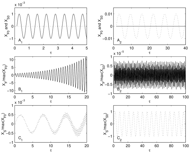
Figure 1: $X_{\text{F}}$ (solid lines) and $X_{\text{F}}$ (dotted lines) plotted against time $\tau$.

When the magnetic field is absent, the system (23)-(24) can be rewritten in the form of a single wave equation. Introducing the new variable:

$$X_{\text{ac}}=k_{x}\hat{u}_{x}+k_{z}\hat{u}_{x},$$ (25)

we can write:

$$\ddot{X}_{\text{ac}}+C_{s0}^{2}k^{2}(1+\delta\cos(\Omega t))X_{\text{ac}}=0,$$ (26)

where the number of dots above the variable indicates the order of time-derivative. This reduction to a single wave equation represents the fact that there are only compressional acoustic waves in the hydrodynamic limit. It is evident that Eq. (26) is a Mathieu-type equation and, thus, an exact analytical solution is available. The solution has a resonant nature when:

$$\Omega\approx 2C_{s0}|k|,$$ (27)

and, more precisely, when the basic frequency of the acoustic wave lies within the following interval

$$\left|C_{s0}|k|-\frac{\Omega}{2}\right|<\left|\frac{\mu}{\Omega}\right|,$$ (28)

where $\mu=\delta C_{s0}^{2}k^{2}$. With this notation, the resonant solution of Eq. (26) takes the following form:

$$X_{\text{ac}}(t)=X_{\text{ac}}(t=0)\exp\left(\frac{\left|\mu\right|}{2\Omega}\tau\right)\left[\cos\left(\frac{\Omega}{2}\tau\right)+\sin\left(\frac{\Omega}{2}\tau\right)\right]$$ (29)

As a conclusion, when the entropy (temperature) oscillates with a frequency that is twice the basic frequency of the acoustic wave, then those waves are resonantly amplified in the system

III.2 Separation of MHD waves

Let us now turn to the general analysis of the system (23)-(24). This system consists of two wave equations which describe the presence of two different wave modes. The velocity fields corresponding to these two kinds of oscillatory motion of the system are clearly coupled. Nevertheless, if one considers a perturbation around a static equilibrium state (i.e. with $\delta=0$), then it is known that appropriate eigenvectors can be constructed which correspond to eigenvalues calculated from the characteristic equation and which are perpendicular to each other. Using this procedure, one can then show that the fundamental modes are separated (or decoupled).

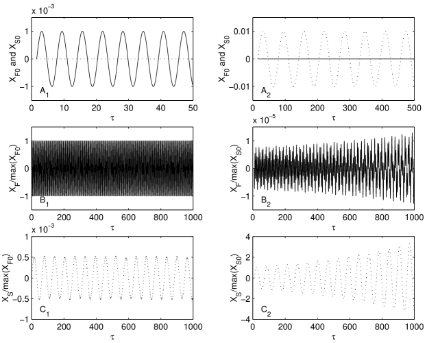
Figure 2: As in Fig. 1 for $\xi\ll 1$.

However, when the background system is driven (i.e. when $\delta\neq 0$), the coefficients in the equations are time dependent. Therefore, the analysis of these equations becomes rather complicated in this case. We are going to construct the ’eigenfunctions’ by employing a similar procedure in combination with numerical techniques, in order to draw a more complete picture of the dynamical processes we are studying here. For this purpose it is convenient to impose an appropriate normalization of the quantities. We introduce the following scaling of the variables: $\hat{U}_{x}=\hat{u}_{x}/V_{A}$, $\hat{U}_{z}=\hat{u}_{z}/V_{A}$, $\tau=V_{A}kt$, $C_{11}=c_{11}/V_{A}k=\xi^{2}K_{x}^{2}+1$, $C_{12}=c_{12}/V_{A}k=\xi^{2}K_{x}K_{z}$, $C_{22}=c_{22}/V_{A}k=\xi^{2}K_{z}^{2}$, here, $K_{i}=k_{i}/k$ ($i=x,z$), $\xi^{2}=C_{s}^{2}/V_{A}^{2}=\xi_{0}^{2}(1+\delta\cos(\hat{\Omega}\tau))$, and $\hat{\Omega}=\Omega/V_{A}k$. Observe that, if we apply an orthogonal transformation on the velocity vector space $(\hat{U}_{x},\hat{U}_{z})$ of the form Courant and Hilbert [1966], Jeffreys and Swirles (1962) [lady Jeffreys]:

$$\begin{array}[]{c}X_{\text{F}}=\cos\theta\hat{U}_{x}-\sin\theta\hat{U}_{z},\\ \\ X_{\text{S}}=\sin\theta\hat{U}_{x}+\cos\theta\hat{U}_{z},\\ \end{array}$$ (30)

where $\theta$ denotes the Euler angle in the velocity space. This transformation is time dependent since the coefficients in the initial matrix:

$$\left(\begin{array}[]{cc}C_{11}&C_{12}\\ C_{12}&C_{11}\\ \end{array}\right)$$ (31)

also depend on time:

$$\tan\theta=\frac{C_{12}}{\Omega_{2}^{2}-C_{11}}=\frac{C_{12}}{C_{22}-\Omega_{1}^{2}}=$$

$$=\frac{C_{11}-\Omega_{1}^{2}}{C_{12}}=\frac{\Omega_{2}^{2}-C_{22}}{C_{12}}.$$ (32)

With this notation, the initial set of equations (23)-(24) can be transformed into:

$$\ddot{X}_{\text{F}}+\left(\hat{\Omega}_{\text{F}}^{2}-\dot{\theta}^{2}\right)X_{\text{F}}=\ddot{\theta}X_{\text{S}}+2\dot{\theta}\dot{X}_{\text{S}},$$ (33)

$$\ddot{X}_{\text{S}}+\left(\hat{\Omega}_{\text{S}}^{2}-\dot{\theta}^{2}\right)X_{\text{S}}=-\ddot{\theta}X_{\text{F}}-2\dot{\theta}\dot{X}_{\text{F}},$$ (34)

where $\Omega_{\text{F}}^{2}$ and $\Omega_{\text{S}}^{2}$ are the eigenvalues of the matrix (31) representing, in fact, the characteristic frequencies of the fast (F) and slow (S) magneto-sonic waves, respectively:

$$\hat{\Omega}_{\text{F},\text{S}}^{2}=\frac{1}{2}\left(C_{11}+C_{22}\pm\sqrt{(C_{11}-C_{11})^{2}+4C_{12}^{2}}\right).$$ (35)

It is well known that in a magnetized plasma there exist three different regimes, which are determined by the relative importance of the thermal and magnetic pressures. This relation usually is parameterized by the ratio of the thermal and magnetic pressures, the plasma beta defined as $\beta=8\pi p_{0}/B_{0}^{2}=\gamma\xi^{2}/2$. The proportionality factor here is of the order of unity. The three regimes are referred to as $\xi^{2}\gg 1$, $\xi^{2}\ll 1$, and $\xi^{2}\simeq 1$, respectively. Accordingly, the basic properties of the different MHD waves are also well studied in these three regimes. Below, we will also consider the problem case by case. Typically below we use $\xi^{2}$ instead of plasma $\beta$.

III.3 The case $\xi^{2}\gg 1$

Firstly, let us consider the limit of large plasma beta. In this case, the magnetization of the plasma is rather weak and the thermal effects dominate in the dynamics of the medium. In this regime, the fast and slow magneto-sonic waves have drastically different properties. In this situation, one obtains from the expressions (35) that

$$\hat{\Omega}_{\text{F}}\gtrsim\xi^{2},$$ (36)

while, on the other hand, the low frequency branch of the spectrum satisfies:

$$\hat{\Omega}_{\text{S}}\lessapprox 1,$$ (37)

showing that the characteristic frequencies of the slow waves lie close to the Alfvén frequency. In general, the fast and slow magneto-sonic modes propagating in an arbitrary, oblique direction with respect to an applied magnetic field are neither purely compressible (longitudinal) nor incompressible (transversal). The latter property relates to the tension of magnetic field lines, like for Alfvén waves. But, both of the wave modes consist of a mixture of these two features. However, when $C_{s}^{2}\gg V_{A}^{2}$, the properties of the fast magneto-sonic waves are very similar to those of sound waves and these waves represent sound waves that are slightly modified by the presence of the magnetic field and the transversal component is weak. Therefore, these waves substantially feel the variation of the sound speed, what directly results in a variable phase speed of the fast modes.

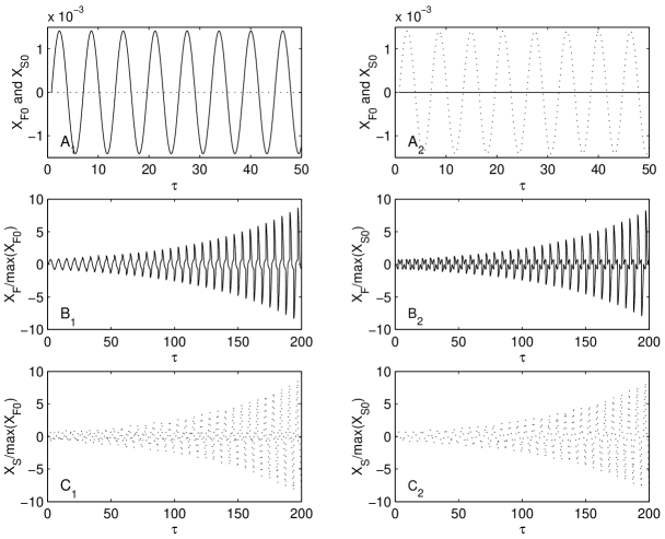
Figure 3: As in Fig. 1 for $\xi=1$. $K_{x}=0.00005$

We now analyze the set of equations (33)-(34) term by term. For this purpose one should use $\delta$ as a small parameter in the problem, as we consider here a nonequilibrium background that is very close to the equilibrium $\delta\ll 1$. We are interested in terms of the order of magnitude up to linear in $\delta$. All higher order terms yield vanishingly small contributions to the considered dynamical process. It can be easily shown that $\hat{\Omega}_{\text{F}}$ includes both zeroth- and first-order terms in the expansion in terms of $\delta$, while the terms $\dot{\theta}$ and $\ddot{\theta}$ do not contain zeroth-order terms and the expansions of both these terms start with the first-order term. Consequently, the term $\dot{\theta}^{2}$ can be neglected in both equations as it consists of terms definitely of second and higher orders in $\delta$. Further, we assume that within the resonance, the fast magneto-sonic wave would be able to grow in amplitude exponentially, while the terms controlling the coupling with the slow waves (on the RHS) are rather small as the characteristic frequencies of these eigenmodes lie far apart from each other according to Eqs. (36)-(37). Consequently, we neglect the coupling terms, which at any rate will be dominated by the terms on the LHS of Eq. (33), and we are left with two approximate ‘decoupled ’equations. With these simplifications, Eq. (33) reduces to:

$$\ddot{X}_{\text{F}}+\hat{\Omega}_{\text{F0}}^{2}\left(1+n_{\text{F}}\cos(\Omega\tau+\varphi_{\text{F}})\right)X_{\text{F}}=0,$$ (38)

where $n_{\text{F}}=n_{\text{F}}(\delta,\Omega)\ll 1$ and $\varphi_{\text{F}}=\varphi_{\text{F}}(\delta,\Omega)$ are the amplitude and the initial phase of the fast wave frequency oscillations in the system, respectively, and $\hat{\Omega}_{\text{F0}}$ is the equilibrium frequency of the fast magneto-sonic waves. This Mathieu-type equation has a resonant solution for the appropriate harmonic of the fast magneto-sonic wave with the frequency (corresponding to a given value of the wavelength):

$$\hat{\Omega}_{\text{F0}}\approx\frac{\Omega}{2},$$ (39)

varying within the interval

$$\left|\hat{\Omega}_{\text{F0}}-\frac{\Omega}{2}\right|<\left|\frac{n_{\text{F}}\hat{\Omega}_{\text{F0}}}{\Omega}\right|,$$ (40)

and reading as:

$$X_{\text{F}}(t)=X_{\text{F}}(\tau=0)\exp\left(\frac{\left|n_{\text{F}}\hat{\Omega}_{\text{F0}}^{2}\right|}{2\Omega}\tau\right)\times$$

$$\times\left[\cos\left(\frac{\Omega}{2}\tau+\varphi_{\text{F}}\right)+\sin\left(\frac{\Omega}{2}\tau+\varphi_{\text{F}}\right)\right].$$ (41)

The approximative analysis, which is given here, should be verified by means of experimental or numerical methods. In the present study, we first concentrate on a rigorous numerical analysis of the initial equations (23)-(24), and then we reconstruct from the results of the numerical simulations, all the relevant quantities we use in the analysis.

Figure 4: As in Fig. figxuni1 for $\xi=1$. $K_{x}=0.5$

Here, we consider two different sets for the initial conditions. First we chose the initial conditions $\hat{U}_{x0}$, $\hat{\dot{U}}_{x0}$, $\hat{U}_{z0}$ and $\hat{\dot{U}}_{z0}$ so that, initially, only the amplitude of the fast magneto-sonic wave (solid line in panel $A_{1}$) is finite and there is no slow magneto-sonic wave in the system (see the dotted line in panel $A_{1}$):

$$X_{\text{S}}(\tau=0)\sim\varepsilon,\hskip 8.5359pt\dot{X}_{\text{S}}(\tau=0)\sim\varepsilon,$$ (42)

where $\varepsilon\approx 10^{-17}$ is the order of magnitude of the numerical error related to the machine precision. Panel $A_{1}$ represents the case of the stationary state in the system ($\delta=0$). On the other hand, in panels $B_{1}$ and $C_{1}$ of the same figure, the curves corresponding to the parameter values $\delta=0.05$ and $\hat{\Omega}_{\text{F0}}=\Omega/2\approx 10$ are plotted. It is obvious that the amplitude of the fast oscillation undergoes a rapid exponential growth in this case (panel $B_{1}$, Fig 1), while the slow magneto-sonic wave is out of resonance and, consequently, its amplitude remains small (panel $C_{1}$). The excitation of this small amplitude slow magneto-sonic disturbance is due to the weak coupling of the fast and slow waves by the external driver. This coupling implies that, even when there is initially no slow magneto-sonic wave, nevertheless, a small amplitude slow magneto-sonic wave perturbation gets excited. These small amplitude vibrations can be referred to as ‘slow’ magneto-sonic noise. The presence of this noise relates to two simultaneous factors, viz. the propagation of the fast magneto-sonic wave and the external driving of the background system. The exclusion of either of these two factors would lead to the disappearance of the slow magneto-sonic perturbation, as is shown in panel $A_{1}$.

On the other hand, we have carried out the simulations for the case when frequency of slow waves satisfies the resonant condition $\hat{\Omega}_{\text{S0}}=\Omega/2\approx 1$. The sound speed yields a negligible contribution into the frequency of the slow magneto-sonic waves, as from expression (37) it is evident that the latter is close to the Alfvén frequency (which in our case is constant), and whatever variations of the sound speed (related to the pressure variation) occur in the system, the slow magneto-sonic wave frequency remains almost unchanged. The corresponding values of the increment $\delta_{S}$ is so small that there is not a significant growth of the slow mode amplitude during any reasonable time span. This means that this variation is not felt by slow magneto-sonic wave modes. In the slow magneto-sonic waves propagating in a high-beta plasma, the incompressible (transversal) component dominates and the properties of these waves are very similar to the purely incompressible Alfvén waves. Therefore, one can expect that the slow magneto-sonic waves (and also the Alfvén waves) do not feel the variations of the sound speed when the Alfvén speed remains constant. This is why, in the case when we initially have only the slow magneto-sonic wave ($A_{2}$ of Fig. 1), these waves stay out of the parametric interaction (panel $C_{2}$), even when an appropriate resonant conditions is formally satisfied. In panel $B_{2}$ of Fig. 1, we plot $X_{\text{F}}$ showing that the fast magneto-sonic wave naturally is out of resonance due to the fact that its frequency is out of the resonant area. Again, the presence of the slow magneto-sonic wave of finite amplitude in the externally driven system leads to the excitation of small amplitude disturbances (panel $B_{2}$), which we can now refer to as ‘fast’ magneto-sonic noise.

To involve the almost incompressible slow magneto-sonic waves into the parametric interaction, one should not consider the case of constant density (for the parametric amplification of Alfvén waves with periodical variation of medium density see Zaqarashvili [2001]). Instead of Eq. (10), the full equation Eq. (6) should then be employed. In that case, the action of the external periodic forces can also be taken into account. However, along with the effect of parametric resonance, we expect that strong couplings between the compressional fast and slow and incompressible Alfvén waves can arise. Therefore, the problem would then not be reducible to two spatial dimensions any more, since the Alfvén speed also would be variable and the Alfvén waves would participate in the process as well. This issue can become the subject of future developments and generalizations of the present model.

III.4 The case $\xi^{2}\ll 1$

In the present subsection, we address the case when the plasma is magnetically dominated, i.e., the case $C_{s}^{2}\ll V_{A}^{2}$. In this regime, the situation is just opposite compared to the previous one. In particular, we know that now the frequency of the fast magneto-sonic wave satisfies

$$\hat{\Omega}_{\text{F}}\gtrsim 1,$$ (43)

and the properties of these waves are close to those of the incompressible Alfvén waves. Consequently, in a low-beta plasma the fast magneto-sonic waves almost do not feel the variation of the entropy. However, this is again true only when an external driver causes a variation of only the pressure while the density remains constant. In general, when the Eq. (6) holds so that the density is variable, the remark given in the previous subsection about the slow magneto-sonic waves and Alfvén waves is now valid for fast magneto-sonic waves.

Within the present framework, the fast magneto-sonic waves stay out of resonance. This can also be discovered by means of numerical simulations. In Fig. 2, we show the results of our simulations for the new set of parameter values in the same order as in Fig 1. Panel $B_{1}$ confirms the validity of the conclusions we have just made.

However, one can again follow an approximative analysis for the slow magneto-sonic waves, in a similar manner as in the previous case. Indeed, contrary to the case of high plasma beta, now the slow magneto-sonic modes are predominantly compressional (longitudinal) and their properties are close to those of the usual sound waves:

$$\hat{\Omega}_{\text{S}}\lesssim\xi^{2}.$$ (44)

Therefore, following a similar logic as before, one can derive an approximate Mathieu-type equation for the slow waves which reads:

$$\ddot{X}_{\text{S}}+\hat{\Omega}_{\text{S0}}^{2}\left(1+n_{\text{S}}\cos(\Omega\tau+\varphi_{\text{S}})\right)X_{\text{S}}=0,$$ (45)

where $n_{\text{S}}=n_{\text{S}}(\delta,\Omega)\ll 1$ and $\varphi_{\text{S}}=\varphi_{\text{F}}(\delta,\Omega)$, respectively, are the amplitude and the initial phase of the slow magneto-sonic wave frequency oscillations in the system, and $\hat{\Omega}_{\text{S0}}$ is the equilibrium frequency of the slow magneto-sonic waves. Again, this Mathieu-type equation has a resonant solution for the appropriate harmonic of the slow magneto-sonic wave with the frequency (corresponding to a given value of the wavelength):

$$\hat{\Omega}_{\text{S0}}\approx\frac{\Omega}{2},$$ (46)

varying within the interval

$$\left|\hat{\Omega}_{\text{F0}}-\frac{\Omega}{2}\right|<\left|\frac{n_{\text{F}}\hat{\Omega}_{\text{F0}}}{\Omega}\right|,$$ (47)

and it has the form:

$$X_{\text{S}}(t)=X_{\text{S}}(\tau=0)\exp\left(\frac{\left|n_{\text{S}}\hat{\Omega}_{\text{S0}}^{2}\right|}{2\Omega}\tau\right)\times$$

$$\times\left[\cos\left(\frac{\Omega}{2}\tau+\varphi_{\text{S}}\right)+\sin\left(\frac{\Omega}{2}\tau+\varphi_{\text{S}}\right)\right]$$ (48)

Furthermore, we verify these findings by a numerical simulation when $\hat{\Omega}_{\text{S0}}=\Omega/2\approx 0.1$. As we show in panel $C_{2}$ of Fig. 2, the slow magneto-sonic waves get amplified, while the fast magneto-sonic waves stay out of resonance (panel $B_{2}$), and the coupling between these waves is again very weak because $\hat{\Omega}_{\text{S0}}\ll\hat{\Omega}_{\text{F0}}$. Observe that in both cases of the initial conditions (panels $A_{1}$ and $A_{2}$), we can see the excitation of the small amplitude ‘slow’ magneto-sonic (panel $C_{1}$) and ‘fast’ magneto-sonic (panel $B_{2}$) noises due to the weak coupling of the waves.

III.5 The case $\xi\approx 1$

This case is of special importance in the problem considered here. When $C_{s}^{2}\approx V_{A}^{2}$, the thermal and magnetic effects are of comparable strength. Under these conditions, the properties of both waves are very similar as:

$$\hat{\Omega}_{\text{F}}\approx\hat{\Omega}_{\text{S}}.$$ (49)

That is the reason why the waves can not only interact with the forced entropy oscillations but, in addition, they also may effectively couple and exchange energy among each other. This can be understood easily if we recall the presence of the terms in the RHS of Eqs. (33)-(34). These equations show that an external driver can effectively couple the waves. This situation is similar to the case of a laminar shear flow in the system Gogoberidze et al. [2004]. As is well-known, the latter also can be maintained only by an external driving of the system. This seems to be a general property of driven systems: the ability to couple eigenmodes of the system under certain conditions. This claim looks apparent in the framework of the current paper. However, a complete and general proof of it can be given only through the general consideration of the fully three-dimensional case when the variability of the background density and the action of the external forces also are taken into account. Here, we should emphasize that the coupling of different kinds of wave modes can be achieved not only with the external driving, which harmonically oscillates in time, but in general, with any kind of driver giving rise to a time dependent entropy (temperature) in the system.

Now, a similar approximative analysis as we have discussed in the previous two cases, would be very ‘rough’. In the case when the waves propagate almost along the magnetic field ($K_{x}\ll 1$), it even becomes completely inapplicable. Consequently, it is convenient to treat the problem in this case only numerically. Before we do this, it is important to emphasize again that the coupling of the different wave modes is possible only because of the presence of the external driving in the system. The simulations show that the dynamics of both wave modes (when the resonant conditions are satisfied) is characterized by the interplay of two different factors. On the one hand, both wave modes are involved in the parametric resonance and, on the other hand, they are effectively coupled to each other.

Let us first consider the case when both fast and slow magneto-sonic modes propagate almost parallel to the magnetic field ($K_{x}\ll 1$). In this case, in 3 we accordingly show the results of the simulations as in the previous subsections. It is apparent that both ‘eigenfrequencies’ lie very close to each other. As a consequence, in Fig. 3 we show that, if initially we have only a fast magneto-sonic wave (panel $A_{1}$) and the resonant condition is satisfied ($\hat{\Omega}=2$), the fast magneto-sonic mode gets amplified via the parametric action (panel $B_{1}$). Besides, the coupling of the two wave modes is very strong in this case and, therefore, the slow magneto-sonic wave is excited and also becomes involved in the amplification process, as this wave satisfies the resonance condition as well (panel $C_{1}$). Both kinds of wave modes effectively exchange energy and the characteristic values of their amplitudes are comparable to each other. The situation is absolutely similar, when initially we set up only a slow magneto-sonic wave (panel $A_{2}$). We then observe that a fast magneto-sonic wave is excited (panel $B_{2}$) and both waves are in parametric resonance with the driver as they exchange energy (panels $B_{2}$ and $C_{2}$). It is important to note that, in this case, the ultimate ‘fate’ of the process is more sensitive to the initial conditions as, contrary to the case of weak coupling, not only the frequencies are important but also their phases matter.

We also investigated the case when the waves propagate in the oblique direction $K_{x}=0.5$. In this case, the frequencies of the modes become somewhat separated even both of them still are of same order of magnitude. Therefore, the coupling effect weakens substantially (as shown in Fig. 4), and the parametric resonance effect only effectively amplifies, with the respective resonant conditions, in the one case only the fast magneto-sonic wave (panel $B_{1}$) and, in the other case, only the slow magneto-sonic wave (panel $C_{2}$). At the same time, it should be noticed that again we discover the generation of the ‘slow’ (panel $C_{1}$) and ‘fast’ (panel $B_{2}$) magneto-sonic noises, which are of much larger amplitude now (as expected) than in the limits of high or low plasma beta.

IV Conclusions

In the present paper we investigated wave motions and wave amplifications in a non-equilibrium setting. In particular, we have developed a model of a magnetohydrodynamic system that is being driven by the combined action of external sources and sinks of heat. More specifically, the external action is a harmonically oscillating function of time. In contrast with many other studies, the background is that of a non-equilibrium state against which we have considered the dynamical properties of the compressional fast and slow magneto-sonic waves. Of special interest has been the case when the external driving of the system results only in a variation of the pressure (or temperature) and it does not lead to a distortion of the background velocity and density fields. A numerical study has led us to the following conclusions:

1. In the hydrodynamic limit ($B_{0}=0$), the spectrum of the possible wave modes reduces to that of the sound waves. In this case, we derived an exact equation, viz. Eq. (26) with an obvious resonant solution given by Eq. (29).

2. In the case of a high beta plasma ($\xi^{2}\gg 1$), the temperature oscillation leads to a major contribution in the variability of the fast magneto-sonic wave frequency $\hat{\Omega}_{\text{F}}$, while the amplitude of the slow magneto-sonic frequency $\hat{\Omega}_{\text{S}}$ oscillation is very small. As a consequence, in this regime only the fast magneto-sonic waves can participate in the parametric resonance with the entropy oscillations (panel $B_{1}$ in Fig. 1) as is predicted by the approximate solution (41). The slow magneto-sonic waves stay out of resonance because the background density (i.e. Alfvén speed) is assumed to be constant (cf. panel $C_{2}$ in Fig. 1), even when the appropriate condition for the parametric resonance is satisfied. Besides, there is a coupling between the fast and slow magneto-sonic waves due to the open nature of the system, as is manifested from the terms on the RHS of Eqs. (33)-(34). This coupling is very weak when the plasma $\beta$ is very large and the frequencies of the waves are very separated. Nonetheless, this coupling leads to the excitation of slow (cf. panel $C_{1}$ in Fig. 1) and fast (cf. panel $B_{2}$ in Fig. 1) “noises” of very small amplitude.

3. The situation is just opposite in the case of low plasma-$\beta$ ($\xi^{2}\ll 1$). In this case only the slow magneto-sonic wave frequency oscillates with the significant amplitude, while the variability of the fast magneto-sonic wave frequency is vanishingly small. Hence, only slow waves can be amplified (cf. panel $C_{2}$ in Fig. 2) by the parametric action of the forced entropy oscillations and the fast magneto-sonic modes do not feel (in the sense of parametric action) these oscillations effectively (cf. panel $B_{1}$ in Fig. 2) with the constant Alfvén speed considered in current work. In addition, we again observe the excitation of slow magneto-sonic (see panel $C_{1}$ in Fig. 2) and fast magneto-sonic (see panel $B_{2}$ in Fig. 2) “noises” due to the weak mode coupling.

4. When ($\xi^{2}\sim 1$), we can distinguish two different situations:

   (i) In the case when both fast and slow magneto-sonic waves propagate almost parallel to the magnetic field $K_{x}\ll 1$, the characteristic frequencies of the different modes are very close to each other. Therefore, there is a strong wave coupling. As a result, there is no possibility for only one kind of wave mode to exist, i.e. the presence of one of the wave modes immediately results in the excitation of the other. In this case, both kinds of waves can be involved together in the parametric resonance as shown in Fig. 3.

   (ii) However, when the waves propagate in the oblique direction with respect to the applied magnetic field, the frequencies become somewhat more separated and then the coupling effect weakens significantly (Fig. 4).

The results obtained in this work can be applied under terrestrial laboratory conditions such as in acoustic investigations but the model also appears useful for the description of some astrophysical processes that are periodic in time, as in objects with a variable intensity of entropy production and losses (as for instance in variable stars). However, at the present stage we aim only to demonstrate the basic physical properties of the parametric amplification of waves and their mutual coupling in nonequilibrium plasmas. Despite of the apparent simplifications our new results are believed to be of general importance and they may have far reaching consequences for many applications. Here follow some possibilities:

• Previous investigations of processes based on parametric resonance in neutral and in conducting fluids have been carried out. These studies have revealed the possibility of an effective parametric amplification of sound waves either due to external mechanical periodic forcing or to mutual nonlinear interactions between the different harmonics of the waves themselves. Along with the references on this matter given in the previous sections, other examples include Silva et al. [2006], Stern and Tzoar [1966], Tokman et al. [2005]. The model outlined in the present work is a unified approach to parametric amplification of sound and of compressional MHD waves in considered two dimensional systems. The generalization to 3D would also enable an experimental treatment of the parametric resonance triggered by an externally driven, oscillating entropy (or temperature). Thus, it would yield a valuable contribution to the rich spectrum of theoretical and experimental studies (for instance, see Rosenbluth [1972], Sugawa and Utsunomiya [1989] and many others) in the field of parametric instabilities in fusion plasmas.

• The spectrum of astrophysical processes, where the considered mechanism of wave amplification and of wave coupling may be useful is even more rich. We have already given (see above) several references concerning the swing (parametric) interactions between different MHD waves in equilibrium magnetic structures, which directly have been applied to the magnetized solar atmosphere. On the other hand, there are many studies, which reveal the importance of parametric resonances at galactic and cosmological scales (for instance, see Easther and Parry [2000], Henriques and Moorhouse [2002], Servin et al. [2000], Zibin et al. [2001]). It should be emphasized that the results obtained in this work may explain the properties of oscillatory phenomena in astrophysical objects being away from thermodynamic equilibrium and sustaining forced entropy oscillations. The entire variety of such thermally variable objects are usually described within the framework of thermal relaxation oscillation theory Wesselink [1939]. We give here references to types of the variable stars which manifest the mentioned oscillatory behavior: Thermal oscillation during the carbon burning Iben [1978] and Helium burning Iben et al. [1986] in the stellar core; Also thermal relaxation in the horizontal-branch stars Salati et al. [1990] and those with convective cores Wood [2000]. In addition, our approach appears interesting for models of globally oscillating coronas Korevaar and Hearn [1989], although such a consideration would require a generalization of the current model for the case when the variability of the density is also taken into account. In such systems the parametric amplification of the physical quantities could even become observable if it would be possible to observe two, mutually related oscillatory processes with the frequencies related as $\omega_{1}\approx 2\omega_{2}$.

The model presented here, of course, requires some further development, e.g. to enable the study of similar effects when the background density and velocity are also variable in time. In addition, the terms corresponding to a perturbation of the source term in the entropy balance equation, due to the propagation of waves, could also be taken into account (in the current model we neglected this term). In that case, additional kinds of modes can arise in the system such as thermal waves and aperiodic vortices which would enrich the spectrum of possible interactions.

*

Appendix A Relation of the heat conduction with the entropy production and its current

The current derivation is based on standard linear response theory for weakly non-equilibrium systems e.g. see Groot and Mazur [1969]. Consider the source term $\lambda\Delta T$ in Eq. (12). It is well known that the coefficient of thermal conduction $\lambda$ arises here due to the assumption that it depends only on the overall equilibrium temperature $\lambda=L_{qq}/T_{00}^{2}$, where $L_{qq}$ is a constant parameter. Setting $L_{qq}=0$ in the considered case reduces the system to the equilibrium. On the other hand, the assumption that the coefficient $\lambda$ is a constant is known as the Fourier approximation, leading to the Fourier law of heat transfer (12). From a general point of view the equation which governs the heat transport reads as:

$$\rho_{0}T_{0}\frac{DS_{0}}{Dt}=\mathbf{\nabla}\cdot\left(\frac{L_{qq}}{T_{0}^{2}}\mathbf{\nabla}T_{0}\right)=-\mathbf{\nabla}\cdot\left(L_{qq}\mathbf{\nabla}\frac{1}{T_{0}}\right)=-\mathbf{\nabla}\cdot\mathbf{j}_{q},$$

which says that the changes in the local entropy are caused by the heat transfer through the system (if there is no source of heat within it). The divergence of the heat current on the r.h.s. can be reorganized as follows:

$$-\mathbf{\nabla}\cdot\mathbf{j}_{q}=T_{0}\left(-\mathbf{\nabla}\cdot\mathbf{j}_{s}+\sigma\right),$$ (50)

which recovers the expression (7) with the microscopic entropy current $\mathbf{j}_{s}=\mathbf{j}_{q}/T_{0}$ and local entropy production

$$\sigma=\mathbf{j}_{q}\cdot\mathbf{\nabla}\left(\frac{1}{T_{0}}\right).$$ (51)

These last equalities reveal the relation between the coefficient of thermal conduction $\lambda$, and the entropy current and its production. As a matter of fact, the presence of the coefficient $\lambda$ in Eq. (12) manifests the presence of both entropy production and its transfer, thus determining the system to be away form thermodynamic equilibrium.

Further, in the Fourier approximation one can write:

$$\sigma_{0}\approx\frac{\lambda^{2}}{L_{qq}}\left(\mathbf{\nabla}T_{0}\right)^{2}$$ (52)

$$-\mathbf{\nabla}\cdot\mathbf{j}_{s}\approx\frac{\lambda\Delta T_{0}}{T_{0}}-\frac{\lambda^{2}}{L_{qq}}\left(\mathbf{\nabla}T_{0}\right)^{2}$$ (53)

These expression can be written explicitly for the example (14):

$$\sigma_{0}\approx\frac{\lambda^{2}T_{01}^{2}}{L_{qq}}f^{2}\exp\left(2fx\right)\exp(2i\omega t),$$ (54)

$$-\mathbf{\nabla}\cdot\mathbf{j}_{s}\approx-\frac{\lambda^{2}T_{01}^{2}}{L_{qq}}f^{2}\exp\left(2fx\right)\exp(2i\omega t)+$$

$$+\frac{\lambda f^{2}T_{01}\exp\left(fx\right)\exp(i\omega t)}{T_{00}+T_{01}\exp\left(fx\right)\exp(i\omega t)},$$ (55)

where,

$$f=\left(-\sqrt{\frac{\omega\rho C_{v}}{2\lambda}}(1-i)\right).$$ (56)

As it has been mentioned in the text we omit the coordinate dependence of these quantities implying that $\exp\left(fx\right)\approx\exp\left(fx_{0}\right)$, where $x_{0}$ is a constant. This last assumption immediately leads to an equation of type (10) with a constant amplitude $\alpha_{1}$, which is under consideration here.

References

- Berktay [1965] H. O. Berktay. Parametric amplification by the use of acoustic non-linearities and some possible applications. Journal of Sound Vibration, 2:462–470, October 1965. doi: 10.1016/0022-460X(65)90123-9.
- Butler and Farrell [1992] K. M. Butler and B. F. Farrell. Three-Dimensional optimal perturbations in viscous shear flow. Phys. Fluids, 4 (A8):1637–1650, August 1992.
- Chagelishvili et al. [1996] G. D. Chagelishvili, A. D. Rogava, and D. G. Tsiklauri. Effect of coupling and linear transformation of waves in shear flows. Phys. Rev. E, 53:6028–6031, June 1996. doi: 10.1103/PhysRevE.53.6028.
- Courant and Hilbert [1966] R. Courant and D. Hilbert. Methods of mathematical physics. Interscience publishers, inc., New York, 1966, 1966.
- Easther and Parry [2000] R. Easther and M. Parry. Gravity, parametric resonance, and chaotic inflation. Phys. Rev. D, 62(10):103503–+, November 2000.
- Gogoberidze et al. [2004] G. Gogoberidze, G. D. Chagelishvili, R. Z. Sagdeev, and D. G. Lominadze. Linear coupling and overreflection phenomena of magnetohydrodynamic waves in smooth shear flows. Physics of Plasmas, 11:4672, October 2004.
- Groot and Mazur [1969] S. R. Groot and P. Mazur. Non-equilibrium thermodynamics. North-Holland publishing company, 1969, 1969.
- Henriques and Moorhouse [2002] A. B. Henriques and R. G. Moorhouse. Cosmic microwave background and parametric resonance in reheating. Phys. Rev. D, 65(10):103524–+, May 2002.
- Iben [1978] I. Iben, Jr. Thermal oscillations during carbon burning in an electron-degenerate stellar core. Astrophys. J. , 226:996–1033, December 1978. doi: 10.1086/156680.
- Iben et al. [1986] I. Iben, Jr., M. Y. Fujimoto, D. Sugimoto, and S. Miyaji. Relaxation oscillations of a helium-burning star - Helium shell flashes not triggered by the accumulation of a critical mass. Astrophys. J. , 304:217–230, May 1986. doi: 10.1086/164155.
- Jeffreys and Swirles (1962) [lady Jeffreys] H. Jeffreys and B. Swirles (lady Jeffreys). Methods of mathematical physics. Cambridge university press, 1962, 1962.
- Korevaar and Hearn [1989] P. Korevaar and A. G. Hearn. Time-dependent corona models - Global relaxation oscillations. A&A, 224:141–152, October 1989.
- Landau and Lifshitz [2004] L. D. Landau and E. M. Lifshitz. Fluid Mechanics - Cource of theoretical physics, volume 6. Amsterdam: Elsevier, 2004, 2nd edition, 2004.
- Lorenz [1963] E. N. Lorenz. Deterministic Nonperiodic Flow. J. Atmos. Sci., 20:130–141, 1963.
- Mansfeld et al. [2003] G. D. Mansfeld, N. I. Polzikova, O. A. Raevskii, and I. G. Prokhorova. Spectrum of parametrically excited bulk acoustic wave composite resonator. In IEEE ultrasonic symposium, pages 1443–1446, 2003.
- Rosenbluth [1972] M. N. Rosenbluth. Parametric Instabilities in Inhomogeneous Media. Physical Review Letters, 29:565–567, August 1972. doi: 10.1103/PhysRevLett.29.565.
- Salati et al. [1990] P. Salati, G. Raffelt, and D. Dearborn. Thermal relaxation oscillations in horizontal-branch stars. Astrophys. J. , 357:566–572, July 1990. doi: 10.1086/168944.
- Servin et al. [2000] M. Servin, G. Brodin, M. Bradley, and M. Marklund. Parametric excitation of Alfvén waves by gravitational radiation. Phys. Rev. E, 62:8493–8500, December 2000.
- Shapiro [1975] B. Shapiro. Parametric interaction processes in acoustical noise. Phys. Rev. B, 12:2402–2411, September 1975. doi: 10.1103/PhysRevB.12.2402.
- Shergelashvili and Poedts [2005] B. M. Shergelashvili and S. Poedts. On the Effect of inhomogeneous Subsurface Flows on High Degree p-Modes. A&A, 438:1083–1097, August 2005.
- Shergelashvili et al. [2005] B. M. Shergelashvili, T. V. Zaqarashvili, S. Poedts, and B. Roberts. “Swing Absorption” of fast magnetosonic waves in inhomogeneous media. A&A, 429:767–777, January 2005. doi: 10.1051/0004-6361:20041494.
- Shergelashvili et al. [2006] B. M. Shergelashvili, S. Poedts, and A. D. Pataraya. Nonmodal Cascade in the Compressible Solar Atmosphere: Self-Heating, an Alternative Way to Enhance Wave Heating. ApJ, 642:L73–L76, May 2006. doi: 10.1086/504350.
- Silva et al. [2006] G. T. Silva, S. Chen, and L. P. Viana. Parametric Amplification of the Dynamic Radiation Force of Acoustic Waves in Fluids. Physical Review Letters, 96(23):234301–+, June 2006. doi: 10.1103/PhysRevLett.96.234301.
- Stern and Tzoar [1966] R. A. Stern and N. Tzoar. Parametric Coupling Between Electron-Plasma and Ion-Acoustic Oscillations. Physical Review Letters, 17:903–905, October 1966. doi: 10.1103/PhysRevLett.17.903.
- Sugawa and Utsunomiya [1989] M. Sugawa and S. Utsunomiya. Analysis of parametric instability of unstable electrostatic ion cyclotron waves in an ion beam-plasma system . Plasma Physics and Controlled Fusion, 31:57–67, January 1989.
- Tokman et al. [2005] I. D. Tokman, G. A. Vugalter, and A. I. Grebeneva. Parametric interaction of two acoustic waves in a crystal of molecular magnets in the presence of a strong ac magnetic field. Phys. Rev. B, 71(9):094431–+, March 2005. doi: 10.1103/PhysRevB.71.094431.
- Trefethen and Embree [2005] L. N. Trefethen and M. Embree. Spectra and pseudospectra, The behavior of nonnormal matrices and operators. Princeton University Press, 2005, 2005.
- Trefethen et al. [1993] L. N. Trefethen, A. E. Trefethen, S. C. Reddy, and T. A. Driscoll. Hydrodynamic stability without eigenvalues. Sci, 261:578–584, 1993.
- Voinovivh et al. [2004] P. Voinovivh, A. Merlen, V. Preobrazhensky, and P Pernod. 2-D numerical simulation of acoustic wave phase conjugation in active medium. In IEEE International ultrasonic, ferroelectrics, and frequency control Joint 50th anniversary conference, pages 1872–1875, 2004.
- Wesselink [1939] A. J. Wesselink. Stellar Variability and Relaxation Oscillations. ApJ, 89:659–668, June 1939.
- Wood [2000] P. R. Wood. Convection-Induced Oscillatory Thermal Modes in Red Giants: A New Type of Stellar Oscillation. In L. Szabados and D. Kurtz, editors, IAU Colloq. 176: The Impact of Large-Scale Surveys on Pulsating Star Research, volume 203 of Astronomical Society of the Pacific Conference Series, pages 379–380, 2000.
- Zaqarashvili [2001] T. V. Zaqarashvili. Swing Amplification of Shear Alfvén Waves through Periodical Density Variations in a Conductive Medium. ApJ, 552:L81–L84, May 2001. doi: 10.1086/320257.
- Zaqarashvili and Roberts [2002] T. V. Zaqarashvili and B. Roberts. Swing wave-wave interaction: Coupling between fast magnetosonic and Alfvén waves. Phys. Rev. E, 66(2):026401, August 2002. doi: 10.1103/PhysRevE.66.026401.
- Zaqarashvili and Roberts [2006] T. V. Zaqarashvili and B. Roberts. Two-wave interaction in ideal magnetohydrodynamics. A&A, 452:1053–1058, June 2006. doi: 10.1051/0004-6361:20053565.
- Zaqarashvili et al. [2002] T. V. Zaqarashvili, R. Oliver, and J. L. Ballester. Parametric Amplification of Magnetosonic Waves by an External, Transversal, Periodic Action. ApJ, 569:519–530, April 2002. doi: 10.1086/339288.
- Zarembo and Serdobolskaia [1975] L. K. Zarembo and O. I. Serdobolskaia. Parametric amplification and generation of sound waves. Akusticheskii Zhurnal, 20:726–732, April 1975.
- Zibin et al. [2001] J. P. Zibin, R. Brandenberger, and D. Scott. Backreaction and the parametric resonance of cosmological fluctuations. Phys. Rev. D, 63(4):043511–+, February 2001.