Appropriate SCF basis sets for orbital studies of galaxies and a ‘quantum-mechanical’ method to compute them

Abstract

We address the question of an appropriate choice of basis functions for the self-consistent field (SCF) method of simulation of the $N$-body problem. Our criterion is based on a comparison of the orbits found in $N$-body realizations of analytical potential-density models of triaxial galaxies, in which the potential is fitted by the SCF method using a variety of basis sets, with those of the original models. Our tests refer to maximally triaxial Dehnen $\gamma-$models for values of $\gamma$ in the range $0\leq\gamma\leq 1$, i.e. from the harmonic core up to the weak cusp limit. When an $N$-body realization of a model is fitted by the SCF method, the choice of radial basis functions affects significantly the way the potential, forces, or derivatives of the forces are reproduced, especially in the central regions of the system. We find that this results in serious discrepancies in the relative amounts of chaotic versus regular orbits, or in the distributions of the Lyapunov characteristic exponents, as found by different basis sets. Numerical tests include the Clutton-Brock (1973) and the Hernquist-Ostriker (1992) basis sets, as well as a family of numerical basis sets which are ‘close’ to the Henquist-Ostriker basis set (according to a given definition of distance in the space of basis functions). The family of numerical basis sets is parametrized in terms of a quantity $\varepsilon$ which appears in the kernel functions of the Sturm-Liouville equation defining each basis set. The Hernquist-Ostriker basis set is the $\varepsilon=0$ member of the family. We demonstrate that grid solutions of the Sturm-Liouville equation yielding numerical basis sets (Weinberg 1999) introduce large errors in the variational equations of motion. We propose a quantum-mechanical method of solution of the Sturm-Liouville equation which overcomes these errors. We finally give criteria for a choice of optimal value of $\varepsilon$ and calculate the latter as a function of the value of $\gamma$, i.e., of the power-law exponent of the radial density profile at the central regions of the galaxy.

1 Introduction

The ‘self-consistent field’ (SCF) method of integrating the gravitational $N$-body problem (Clutton-Brock 1972, 1973; Aoki & Iye 1978; Allen, Palmer & Papaloizou 1990; Hernquist & Ostriker 1992; Earn and Sellwood 1995; Weinberg 1999) has so far proved quite useful in the study of particular classes of stellar systems such as isolated galaxies. A powerful characteristic of this method is that the gravitational potential, or the force field, at any point of the particles’ configuration space are rendered by the code in a closed mathematical form, expressed as a series in a suitable set of basis functions. The main task of the code is to calculate the coefficients of a series, the resulting potential of which (say $V(r,\theta,\phi)$ in spherical coordinates) corresponds, via Poisson equation $\nabla^{2}\Phi=4\pi G\rho$, to a smooth density field $\rho(r,\theta,\phi)$ that is the continuous limit of the mass distribution of the $N$ particles. For a known such distribution $\rho(r,\theta,\phi)$, the series coefficients are given by definite volume integrals of quantities depending on both $\rho(r,\theta,\phi)$ and on the basis functions. In a $N$-body simulation, however, we do not have a priori knowledge of the smooth limit $\rho(r,\theta,\phi)$. Thus, we can only obtain Monte Carlo estimates of the values of the coefficients based on the particles’ positions, i.e., mass elements $dm=\rho(r,\theta,\phi)r^{2}\sin\theta drd\theta d\phi$ are replaced in all the volume integrals by point masses (= the particles) and the integrals are approximated by sums over the particles’ positions. It follows that the overall complexity of the SCF method is $O(N)$, i.e. linear on the number of particles. Parallelization is straightforward (Hernquist, Sigurdsson & Bryan 1995) and applications involving $10^{6}$ - $10^{9}$ particles are tractable on present-day computers.

Owing to its nature, the SCF method is particularly suitable to the purpose of studying the orbital structure or the global dynamics of self-consistent models of galaxies. In general, there are three ways of producing smooth estimates of the potential of a self-consistent stellar dynamical system:

a) One chooses an ‘ad hoc’ analytical model for the potential and then produces a Schwartzchild-type (1979) self-consistent model based on a large number of orbits. In this case we actually make no estimate but simply specify the potential in advance. Thus the orbital analysis is relatively easy (see Efthymiopoulos, Voglis & Kalapotharakos 2007, section 4 for an indicative list of references) since it only requires to integrate orbits in a fixed potential. However, it is well known that the self-consistent models constructed by Schwartzchild’s method are non-unique, as many different models can be constructed for the same system which vary in the velocity distribution. Furthermore, the stability of the Schwartzchild-type models cannot be a priori guaranteed (Merritt 1999; Efthymiopoulos et al. 2007).

b) One makes an $N$-body simulation using one numerical method (e.g. direct summation, TREE, or mesh code) up to a final time, e.g., when the system reaches equilibrium. Then one obtains a smooth estimate of the potential at the final snapshot using a different method, for example, spline interpolation, fitting with polynomial or rational functions, grid or the SCF method. When possible, this method is to be preferred over Schwartzchild’s method since $N$-body equilibria are by definition self-consistent and also stable. An important early example was given by Sparke and Sellwood (1987) in the case of a fast rotating barred galaxy, while more recent examples, in the case of elliptical galaxies, were given by Contopoulos, Efthymiopoulos & Voglis 2000; Jesseit, Naab & Burkert 2005; Muzzio, Carpintero & Wachlin 2005 and Muzzio 2006. Attention should however be paid on that the use of two different methods to fit the potential, during and after the $N$-body evolution, may introduce discrepancies in the resulting analysis of the orbits. The sensitivity of the orbital analysis on the potential approximation was studied by Carpintero and Wachlin (2006). These authors found that the relative amount of chaotic versus regular orbits in a stationary triaxial model depends significantly on the way chosen to approximate the potential. As shown in the sequel (sections 3 and 4), this occurs even if two approximations are similar, e.g., in the case of the SCF method, two not very different basis sets. This can be due, for example, to the form of the basis functions, when this does not fit the morphology of the galaxy, or to errors introduced in the equations of motion, when a basis set is numerically calculated on a grid (as suggested by Weinberg 1999). In any case, such numerical effects affect the orbital analysis in such a way that it becomes unclear up to what extent the orbital structure found in a particular system should be attributed to the real dynamics of the system or to numerical features of the code that fits the potential.

c) One integrates the $N$-body system as in (b) and then uses the same scheme (provided by the $N$-body code) to fit the potential at the final snapshot after the $N$-body run (Pfenniger and Frendli 1991, Udry and Martinet 1994, Holley-Bockelmann et al. 2001, 2002; Contopoulos, Voglis & Kalapotharakos 2002; Voglis, Kalapotharakos & Stavropoulos 2002; Athanassoula 2002, Kalapotharakos, Voglis & Contopoulos 2004; Shen & Sellwood 2004; Kalapotharakos & Voglis, 2005; Voglis, Stavropoulos & Kalapotharakos 2006). This method has internal consistency to a larger degree than (a) or (b). The SCF method is an obvious candidate for such simulations. Nevertheless, as already pointed out, the true ‘smooth’ limit of the distribution of the $N$ particles in an actual $N$-body simulation is not known a priori (the precise meaning of such a limit has even been questioned in the literature, Gurzandyan and Savvidy 1986, Kandrup & Sideris 2003). Thus, the question still remains on how credible can the reproduction of the orbital structure of an ideally smooth gravitational system be, when using an SCF method to fit the potential that is based solely on data of a discretized version of the system, i.e., of the $N$-body system. A second relevant question is whether there are means that can be devised so that this credibility be maximized. In the present paper we deal, precisely, with the above two questions, focusing our investigation, as regards in particular the second question, on the appropriate choice of basis functions for the SCF method and on an appropriate method to calculate them (when they are not given analytically).

We propose the following as a numerical test checking the credibility of a particular SCF method (or of any other potential fitting method): 1) Choose a pair of smooth potential-density functions $\rho(\mathbf{r}),\Phi(\mathbf{r})$. 2) Create an $N$-body realization of the distribution $\rho(\mathbf{r})$ (this can be done by the Monte-Carlo method). 3) Use the SCF code (or any other code) in order to calculate a numerical estimate of the smooth potential $\Phi_{NB}(\mathbf{r})$ from the $N$-body system. This we call the response potential. 4) Finally, compare the orbital structures of the two systems defined by the potentials $\Phi(\mathbf{r})$, $\Phi_{NB}(\mathbf{r})$. The code can be characterized as reliable if the two potentials yield a similar orbital structure. Besides the orbits themselves, a comparison may involve various quantities characterizing the orbital dynamics such as, for example, the calculation of the profile of the forces, frequency analysis of the orbits, Poincaré phase plots, Lyapunov characteristic exponents or other indicators of chaos, etc. Our comparisons in the present refer to the central profiles of the forces and to the distributions of the Lyapunov characteristic exponents of the orbits. We also give estimates of the impact of Poisson noise, introduced at step (2), on the results. The impact of discreetness was examined in a somewhat different context by Holley-Bockelmann, Weinberg & Katz (2005).

We focus on models of elliptical galaxies, in which an important factor affecting the accuracy of the potential fitting is the choice of basis functions for the radial part of the potential expansion (Hernquist & Ostriker 1992; Hozumi & Hernquist 1995). This is related to the fact that the orbits in such systems are sensitive especially on the radial profile of the forces in the central parts of the galaxy. On the basis of their central luminosity profiles, the elliptical galaxies are distinguished in two groups (Ferarrese et al. 1994; Lauer et al. 1995): a) the ‘core’ galaxies, with nearly flat or ‘shallow’ surface brightness profiles, corresponding to power-law density profiles $\rho(r)\propto r^{-\gamma}$ with $0\leq\gamma\lesssim 1$ (Fridman & Merritt 1997), and b) the ‘power-law’ galaxies in which $\gamma\geq 1$, which are further categorized into those with a ‘weak cusp’ ($\gamma\simeq 1$) or ‘strong cusp’ (($\gamma\simeq 2$) (Merritt & Fridman 1996). In case (a) the force at the centre is equal to zero, while in case (b) the force is finite, for $\gamma=1$, or infinite, for $\gamma>1$. These differences in the force field at the centre affect directly the regular or chaotic character of the orbits (see Efthymiopoulos et al. 2007 for a review), and imply that a SCF method can only be successful if it reproduces correctly the central behavior of the forces. In addition, examples are given in which small numerical errors in the potential are amplified in the forces, i.e., derivatives of the potential, and even more in the variational equations, i.e., second derivatives of the potential, through which the Lyapunov characteristic exponents of the orbits are evaluated. We find that this may lead to an erroneous characterization especially of the regular or chaotic character of the orbits. Furthermore, even if an error appears in only a small central region, its presence can affect a large number of orbits, in particular box orbits which pass arbitrarily close to the centre. Since the box orbits constitute the backbone of many elliptical galaxies, the dynamical implications of differences in the central force field are important at least in these galaxies. This we check by taking as our basic model a maximally triaxial Dehnen (1993) $\gamma-$model (Merritt & Fridman 1996) for values of $\gamma$ in the range $0\leq\gamma\leq 1$, i.e., from the limit of a harmonic core up to the ‘weak cusp’ limit. Such cases are characterized by the presence of many box orbits, and indeed, we find that these orbits are strongly affected by the SCF basis set used to obtain the response potential, mainly because of differences in the central force field. This contradicts a claim by Hernquist & Ostriker (1992, section 5.2.1) that such differences are “probably not significant from a dynamical point of view”.

In our tests we consider radial basis sets obtained from the literature, i.e., the Hernquist-Ostriker (1992) and the Clutton-Brock (1973) basis sets, but also a family of basis sets computed numerically, as proposed by Weinberg (1999). In computing the latter, however, we did not use a grid method to solve the associated Sturm-Liouville boundary value problem (Pruess and Fulton 1993) because we demonstrate that such methods often result in large errors appearing in the variational equations of motion which make use of the second derivatives of a specified basis set (section 3). Instead, we propose a ‘quantum-mechanical’ method of solution of the Sturm-Liouville problem which overcomes these errors. This method is applicable when the Sturm-Liouville differential equation to be solved is ‘close’ to another differential equation for which the solution is known analytically (the definition of distance of two differential operators is given in section 3). In our examples below we use the ‘quantum-mechanical’ method in order to calculate numerical basis sets which are ‘close’ to the Hernquist-Ostriker (1992) basis set, but improve, however, the representation of the forces at the central parts of the galaxy. The family is parametrized by a quantity $\varepsilon$ which appears in the Sturm-Liouville differential equation (the Hernquist-Ostriker basis set is the $\varepsilon=0$ member of the family). We then explore which member of the family better fits, in the $N$-body realization, the true dynamics of the Dehnen model for a particular value of $\gamma$. The latter information is given in terms of a function $\varepsilon(\gamma)$ specifying, essentially, the choice of optimal basis set as a function of the power-law exponent $\gamma$ of the central density profile of the galaxy (when $\gamma\leq 1$). This information can be used a priori, i.e., one may choose the optimal basis set for a given $N$-body simulation by measuring first the value of $\gamma$ (from the $N$-body data).

The paper is organized as follows: section 2 presents the general formalism of the SCF method in spherical coordinates, following the same notation as in Weinberg (1999), and then refers to the appearance of errors due to several previously mentioned sources. Section 3 describes our ‘quantum-mechanical’ method of determination of numerical basis sets. Section 4 contains the main results regarding the choice of an optimal basis set following a comparison of the orbits in various Dehnen models and in their respective $N$-body response models. Section 5 summarizes the main conclusions of the present study.

2 The Method

2.1 Basic Formalism of the SCF method

We start with the basic formalism of the self-consistent field method in the case of spherical coordinates, following the same notation as in Weinberg (1999) for cylindrical coordinates. In the SCF approach, a distribution of particles in ordinary space is viewed as a Monte Carlo realization of a smooth density field. This field, which is a continuous and differentiable function in space and time is given by the integration of the distribution function $f$ with respect to the velocities:

$$\rho(\mathbf{r},t)=\int_{\mbox{velocities}}f(\mathbf{r},\mathbf{v},t)d^{3}\mathbf{v}.$$ (1)

In the sequel we fix the value of the time $t$ and drop this from the arguments of $\rho$. In the SCF method the function $\rho(\mathbf{r})$ is expanded in a truncated series of basis functions in coordinates relevant to the shape of the system under study. In the case of elliptical galaxies the usual choice are multipole expansions in spherical coordinates. Let $\rho_{monopole}(r)$ be the monopole term of the multipole expansion of the density and $\rho_{00}(r)$ a rough estimate that we make of it. Then, we express the monopole term as a truncated series in terms of radial basis functions $u_{n00}(r)$, i.e.:

$$\rho_{monopole}(r)=\rho_{00}(r)\sum_{n=0}^{n_{max}}b_{n00}u_{n00}(r).$$ (2)

The use of a discrete spectrum of basis functions $u_{n00}(r)$ (labelled by the ‘radial quantum number’ $n$) follows from boundary conditions imposed to the system (e.g. finite total mass and/or finite size). The coefficients $b_{n00}$ are unknown and the main task of the $N$-body code is to specify their values. Eq.(2) reflects our expectation that a linear combination of the functions $u_{n00}(r)$ can fit the residuals of the true monopole term of the real density with respect to our initial estimate $\rho_{00}(r)$ which acts as an envelope in front of the sum in the r.h.s.. In reality, the fitting is efficient if only a small number of terms are needed in (2) (the uppermost limit of $n$, imposed by the $N$-body resolution is $n_{max}=O(N^{1/3})$ but in practice we use a number of terms which is one order of magnitude smaller than this limit (Palmer 1994)). This, on its turn, depends crucially on the initial estimate $\rho_{00}(r)$, which appears not only directly in Eq.(2) but also, as shown below, indirectly, through the Sturm-Liouville differential equation which specifies the basis functions $u_{n00}(r)$. At any rate, in the same way as for the monopole term, we can make in advance some estimate of the profile of the multipole terms of the density by choosing estimate functions $\rho_{lm}(r)$ and then fit the residuals of the true multipole terms with respect to the functions $\rho_{lm}(r)$ via series in respective basis functions $u_{nlm}(r)$. That is, the density is finally written as:

$$\rho(r,\theta,\phi)=\sum_{l=0}^{l_{max}}\sum_{m=-l}^{l}\sum_{n=0}^{n_{max}}b_{nlm}\rho_{lm}(r)u_{nlm}(r)Y_{l}^{m}(\theta,\phi)$$ (3)

where $Y_{l}^{m}(\theta,\phi)$ are spherical harmonics (e.g. Binney and Tremaine 1987, pp.655-656). Similarly as for the monopole term, the coefficients $b_{nlm}$ are unknown while the functions $u_{nlm}(r)$ are specified in advance via solutions of a Sturm-Liouville differential equation in which the functions $\rho_{lm}(r)$ also appear.

The determination of the basis set of functions $u_{nlm}(r)$ is done as follows: Repeating for the gravitational potential the same procedure as for the density, i.e., selecting in advance some estimate functions $\Phi_{lm}(r)$ for the profiles of the various multipole potential terms we also write the potential as

$$\Phi(r,\theta,\phi)=\sum_{l=0}^{l_{max}}\sum_{m=-l}^{l}\sum_{n=0}^{n_{max}}c_{nlm}\Phi_{lm}(r)u_{nlm}(r)Y_{l}^{m}(\theta,\phi)$$ (4)

with unknown coefficients $c_{nlm}$, and then match Eqs.(3) and (4) via Poisson equation. This yields finally (in units in which $G=1$):

$$-\dfrac{d}{dr}\left(r^{2}\Phi_{lm}^{2}\dfrac{du_{nlm}}{dr}\right)+\left[l(l+1)\Phi_{lm}^{2}-\Phi_{lm}\dfrac{d}{dr}\left(r^{2}\dfrac{d\Phi_{lm}}{dr}\right)\right]u_{nlm}=-(4\pi\lambda_{nlm}r^{2}\Phi_{lm}\rho_{lm})u_{nlm}$$ (5)

with $\lambda_{nlm}=b_{nlm}/c_{nlm}$. Equation (5), supplemented with appropriate boundary conditions, is a case of the Sturm-Liouville eigenvalue problem

$$-\dfrac{d}{dr}\left[p_{lm}(r)\dfrac{du}{dr}\right]+q_{lm}(r)u=\lambda w_{lm}(r)u$$ (6)

with

$$p_{lm}(r) =r^{2}\Phi_{lm}^{2}(r)$$ (7a)

$$q_{lm}(r) =l(l+1)\Phi_{lm}^{2}(r)-\Phi_{lm}(r)\frac{d}{dr}\left(r^{2}\frac{d\Phi_{lm}(r)}{dr}\right)$$ (7b)

$$w_{lm}(r) =-4\pi r^{2}\Phi_{lm}(r)\rho_{lm}(r).$$ (7c)

From the form of (5) it follows that the functions $u_{nlm}(r)$ are given by the eigenfunctions of a Sturm-Liouville differential operator

$${\cal L}_{lm}=-\frac{d}{dr}\left[p_{lm}(r)\frac{d}{dr}\right]+q_{lm}(r)$$ (8)

acting on functions belonging to a Hilbert space with the inner product definition

$$<f|g>=\int_{r_{a}}^{r_{b}}f(r)g(r)w_{lm}(r)dr~{}~{}$$ (9)

where $r_{a},r_{b}$ are two radii at which boundary conditions must be given in the form (Pruess & Fulton 1993)

$$a_{1}u-a_{2}\left(p_{lm}(r)\frac{du}{dr}\right) =\lambda_{nlm}\left(a_{1}^{\prime}u-a_{2}^{\prime}\frac{du}{dr}\right)~{}~{}~{}~{}\mbox{at}~{}r=r_{a}$$ (10a)

$$b_{1}u+b_{2}\left(p_{lm}(r)\frac{du}{dr}\right) =0~{}~{}~{}~{}~{}~{}~{}~{}~{}~{}~{}~{}~{}~{}~{}~{}~{}~{}~{}~{}~{}~{}~{}~{}~{}~{}~{}~{}~{}~{}\mbox{at}~{}r=r_{b}$$ (10b)

with constants $a_{1},a_{2},a_{1}^{\prime},a_{2}^{\prime},b_{1},b_{2}$. The problem admits a discrete set of solutions, i.e., a discrete set of eigenvalues $\lambda_{nlm}$ and eigenvectors $u_{nlm}$, $n=0,1,2,...$ of ${\cal L}_{lm}$. In this way, the basis functions $u_{nlm}(r)$ are specified by the initial choice of estimate functions $\rho_{lm}(r),\Phi_{lm}(r)$, which are hereafter called the kernel functions of the Sturm-Liouville problem, and by the boundary conditions. The index $n$ is called the radial quantum number.

In galactic problems, the radii $r_{a},r_{b}$ are usually set equal to $r_{a}=0$ (centre of the system), and $r_{b}=R_{p}$ or $r_{b}\rightarrow\infty$, depending on whether we consider a system ending at a finite radius $R_{p}$ or at infinity. In the former case, the boundary conditions at $r_{b}=R_{p}$ represent the request of continuity, and of continuous derivative, of the potential function at the point $R_{p}$ where we pass from Poisson to Laplace equation. Such boundary conditions can always be cast in the form (10).

If the kernel functions $\Phi_{lm}(r)$, $\rho_{lm}(r)$ satisfy Poisson equation $\nabla^{2}\Phi_{lm}(r)=4\pi G\rho_{lm}(r)$, then they are called a potential-density pair of functions. In that case we always have $\lambda_{0lm}=1$ and $u_{0lm}=const$. Independently of whether the kernel functions are potential-density pairs or not, the eigenfunctions $u_{nlm}(r)$ of the Sturm-Liouville problem (5) are always orthogonal with respect to the inner product definition (9).

In an $N$-body simulation we use the above formalism in order to obtain a smooth potential function as follows:

a) We specify in advance the sets $\rho_{lm}(r)$, $\Phi_{lm}(r)$, and then $u_{nlm}(r),\lambda_{nlm}$, as explained above.

b) Given the particles’ positions, we find estimates of the coefficients $b_{nlm}$ of an underlying ‘smooth’ density field, by exploiting the orthogonality relation $<u_{nlm}|u_{n^{\prime}lm}>=\delta_{n,n^{\prime}}$, together with the orthogonality of the spherical harmonic functions. Namely, equation (3) is inverted, yielding the value of any particular coefficient $b_{nlm}$ as

$$b_{nlm}=\int_{r_{a}}^{r_{b}}\int_{0}^{\pi}\int_{0}^{2\pi}R(r,\theta,\phi)drd\theta d\phi$$ (11)

where

$$R(r,\theta,\phi)=-4\pi\Phi_{lm}(r)u_{nlm}(r)Y_{l}^{m*}(\theta,\phi)\rho(r,\theta,\phi)r^{2}\sin\theta.$$

Assuming now that the positions of the $N$ particles provide a discrete realization of the smooth density field $\rho(r,\theta,\phi)$, the volume integral (11) can be evaluated by the Monte Carlo method, i.e., as a sum over the particles’ positions:

$$b_{nlm}\simeq\sum_{i=1}^{N}-4\pi\Phi_{lm}(r_{i})u_{nlm}(r_{i})Y_{l}^{m*}(\theta_{i},\phi_{i}).$$ (12)

c) We finally calculate the coefficients of the potential series as $c_{nlm}=b_{nlm}/\lambda_{nlm}$.

The use of a discrete sum instead of a continuous integration implies that, contrary to what the term ‘smooth field’ might suggest, there is always some numerical noise in the system introduced by discreteness effects, which produces ‘relaxation’ effects in the $N$-body simulation (see Palmer 1994, or Weinberg 1996 for a detailed discussion). In our numerical examples in the sequel we examine in detail the effect of this type of noise on the orbits. At any rate, as already mentioned the goodness of the fit of the smooth potential of a system by the SCF series depends crucially on the choice of basis functions $u_{nlm}$ which, on their turn, depend on the choice of appropriate kernel functions $\rho_{lm}(r)$, $\Phi_{lm}(r)$. To this we now turn our attention.

2.2 The choice of basis functions

In order to determine a suitable basis set, a common strategy in the literature is to use kernel functions $\rho_{lm}(r)$, $\Phi_{lm}(r)$ such that the solutions of (5) are reduced to some simple form given, e.g., in terms of special functions or in a closed polynomial form. We mention the following examples (see Hernquist & Ostriker 1992 for a detailed review):

(i) the Clutton-Brock (1973, hereafter CB) set. The kernel functions are:

$$\rho_{lm}(r) =\frac{\sqrt{4\pi}}{4\pi}(2\,l+1)(2\,l+3)\dfrac{a^{2}\,r^{l}}{(a^{2}+r^{2})^{l+5/2}}$$ (13a)

$$\Phi_{lm}(r) =-\sqrt{4\pi}\dfrac{r^{l}}{(a^{2}+r^{2})^{l+1/2}}$$ (13b)

with boundary conditions

$$\left.\dfrac{du_{nlm}(r)}{dr}\right|_{r=0}=0\text{~{}~{}and~{}~{}}\lim_{r\rightarrow\infty}\dfrac{du_{nlm}(r)}{dr}=0.$$

In the form (10) these conditions are given e.g. as $a_{1}=a_{1}^{\prime}=a_{2}^{\prime}=0$, $a_{2}=1$, and $b_{1}=0$, $b_{2}=1$. The zeroth order term of the density expansion

$$\rho_{000}=\frac{3}{\sqrt{4\pi}}\frac{a^{2}}{(a^{2}+r^{2})^{5/2}}$$

yields a half-mass radius equal to unity, $r_{1/2}=1$, if $a\simeq 0.77\simeq 10/13$. The corresponding potential is

$$\Phi_{000}=-\sqrt{4\pi}\frac{1}{(a^{2}+r^{2})^{1/2}}.$$

The above set $\rho_{000},\Phi_{000}$ is the well known Plummer model. The eigenfunctions $u_{nlm}(r)$ are Gegenbauer polynomials of the form $C_{n}^{l+1}(\xi)$ (independent of $m$) where $\xi=\dfrac{r^{2}-a^{2}}{r^{2}+a^{2}}$.

(ii) the set of Allen et al. (1990). In this case there are no kernel functions of the potential or density, i.e.

$$\rho_{lm}(r)=1,~{}~{}~{}\Phi_{lm}(r)=-1.$$ (14)

The inner boundary condition is $du_{nlm}(0)/dr=0$ while the outer boundary condition corresponds to the matching of the solutions of the Poisson and Laplace equations at some finite radius $r_{b}=R_{p}$

$$\left.\dfrac{du_{nlm}(r)}{dr}\right|_{r=0}=0,~{}~{}~{}\left.r\dfrac{du_{nlm}(r)}{dr}+(l+1)u_{nlm}(r)\right|_{r=R_{p}}=0.$$

In the form (10) we set $a_{1}=a_{1}^{\prime}=a_{2}^{\prime}=0$, $a_{2}=1$, and $b_{1}=l+1$, $b_{2}=1/R_{p}$. The eigenfunctions $u_{nlm}(r)$ are spherical Bessel functions. This set better fits systems with a harmonic core.

(iii) the Hernquist-Ostriker (1992, hereafter HO) set. The kernel functions are

$$\rho_{lm}(r) =\sqrt{4\pi}\dfrac{1}{2\pi}\dfrac{(2l+1)(l+1)}{r}\dfrac{a\,r^{l}}{(a+r)^{2l+3}}$$ (15a)

$$\Phi_{lm}(r) =-\sqrt{4\pi}\dfrac{r^{l}}{(a+r)^{2l+1}}.$$ (15b)

The zeroth order term of the density

$$\rho_{000}(r)=\sqrt{4\pi}\frac{1}{2\pi}\frac{1}{r}\frac{a}{(a+r)^{3}}$$

yields a half-mass radius equal to unity, $r_{1/2}=1$, if $a=(1+\sqrt{2})^{-1/2}$ which is our choice of value of $a$ in the sequel. The boundary conditions are $\dfrac{du_{nlm}}{dr}=\mbox{finite}$ at $r_{a}=0$ and the same as in the CB set at infinity. In the form (10) we give precisely the same constants as in the CB set. The eigenfunctions $u_{nlm}$ are Gegenbauer polynomials of the form $C_{n}^{2l+\frac{3}{2}}(\xi)$ where $\xi=\dfrac{r-a}{r+a}$.

The choice of an appropriate set of basis functions is related to the morphological characteristics of the system under study. For example, if the kernel function $\rho_{00}(r)$ is selected as in the HO basis set (Eq.(15a)), this function yields a power-law cusp $\rho_{00}(r)\sim r^{-1}$at the centre, so the HO set cannot easily fit systems in which the density cusp at the centre is shallower than this law. In fact, Hernquist & Ostriker (1992, subsection 2.3) give an idealized example in which a flat profile at the centre can be represented by a linear combination of the $n=0$ and $n=1$ monopole terms of the HO basis set, because the coefficients of these terms are balanced in a way so as to eliminate the power-law dependence $r^{-1}$. However, we can show that if, due, for example, to the Poisson noise, the balance is slightly distorted in an actual $N$-body calculation, the $r^{-1}$ singular behavior of the density at the centre reappears as a result of the numerical error. In our normalization units and constants ($a=(1+\sqrt{2})^{-1/2}$, which corresponds to $a=1$ in Hernquist & Ostriker 1992), the example refers to the spherical density profile:

$$\rho_{0}(r)={3\over 4\pi}{a\over(a+r)^{4}}$$ (16)

which is clearly flat at the centre. While the kernel function $\rho_{00}(r)$ given by Eq.(15a) goes as $\rho_{00}(r)\sim r^{-1}$ at the centre, a combination of the two first monopole terms of the radial basis set allows one to remove the singularity and obtain the profile (16). Precisely, we have:

$$u_{nlm}={a^{l+{1\over 2}}2^{4l+3}\Gamma(2l+{3\over 2})\over 4\pi}\sqrt{n!(n+2l+{3\over 2})\over(1+2l)(l+1)\Gamma(n+4l+3)}C_{n}^{2l+\frac{3}{2}}\left(\frac{r-a}{r+a}\right)$$ (17)

so that

$$\rho_{000}={\sqrt{3}a^{3/2}\over 2\pi r(a+r)^{3}}$$

and

$$\rho_{100}={\sqrt{15}a^{3/2}(r-a)\over 2\pi r(a+r)^{4}}.$$

Thus

$$\rho_{000}(r)+c\rho_{100}(r)={\sqrt{3}a^{3/2}\over 2\pi r(a+r)^{3}}\Bigg{[}1+{c\sqrt{5}(r-a)\over r+a}\Bigg{]}$$

and, if $c=1/\sqrt{5}$ (which corresponds to $c=1/12$ in the units of Hernquist & Ostriker (1992)), we find

$$\rho_{000}+{1\over\sqrt{5}}\rho_{100}={\sqrt{3}a^{3/2}\over\pi(a+r)^{4}}\propto\rho_{0}(r).$$ (18)

However, the balance in Eq.(18) is quite sensitive to numerical errors. For example, if, due to discreteness effects, there is a small error $\epsilon_{0}$ in the ratio $c$ of the numerical coefficients of $\rho_{000}$ and $\rho_{100}$, i.e., $c=1/\sqrt{5}+\epsilon_{0}$, the error introduced in the evaluation of the density is

$$\rho_{000}+({1\over\sqrt{5}}+\epsilon_{0})\rho_{100}=\rho^{\prime}_{0}(r)={\sqrt{3}a^{3/2}\over\pi(a+r)^{4}}+{1\over r}\Bigg{(}{3\epsilon_{0}(r-a)\over 8\pi(a+r)^{4}}\Bigg{)}$$ (19)

and we have $\lim_{r\rightarrow 0}\rho^{\prime}_{0}(r)=\infty$, i.e. the density as calculated by the SCF method with the HO basis set becomes singular at the centre.

Fig. 1 shows a numerical calculation of the above effect. Using a $(50\times 100\times 200)$ spherical polar grid in $(\theta,\phi,r)$ respectively, logarithmic in the radii (from $r=0$ to $r=15$), and linear in the angles, we produced an $N$-body realization of the spherical system (16) with $N=1.25\times 10^{7}$ particles as follows: a) a theoretical value of the number of particles in each grid cell was calculated, that is given by $\Delta N_{th}=\rho_{0}(r_{c})r_{c}^{2}\sin\theta_{c}\Delta r\Delta\theta\Delta\phi$, where $r_{c},\theta_{c}$ are the values of $r$ and $\theta$ at the centre of the cell. b) A random integer number $\Delta N$ is then determined which has a Poisson distribution corresponding to a mean value $<\Delta N>=\Delta N_{th}$ and dispersion $\sigma=\Delta N_{th}^{1/2}$. c) The values $\Delta N$ for all the cells were normalized so that the total number of particles is kept equal to $N$. d) Each cell was filled with $\Delta N$ particles located randomly within the cell with a uniform distribution. Finally, we used this distribution of particles to calculate the coefficients of the ten first monopole terms $b_{n00}$, $n=0,\ldots,9$, of the sum (2) with the HO basis set.

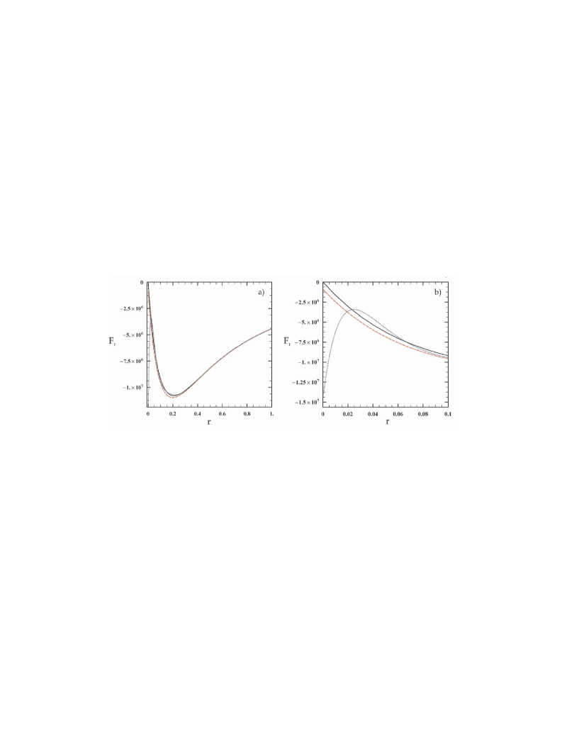
Figure 1: (a) The profile of the radial force $F_{r}(r)$ corresponding to a mass distribution with the density profile (16) (with $1.25\times 10^{7}$ particles) as derived analytically (solid curve) and via the SCF calculation by the first two monopole functions ($n=0,1$, $l=m=0$) (dashed red curve) and by the first ten monopole functions ($n=0-9$, $l=m=0$) (dotted blue curve) of the HO radial basis set implemented on an $N$-body realization of this mass distribution (see text for details). (b) A zoom of (a) in the central region of the model. For large radii the force is represented very good in both cases (two and ten monopole terms expansion). For small radii the first two monopole terms yield a small but definitely finite value of the force at $r=0$ while the first ten monopole terms yield a conspicuous error in the force near the centre $r=0$.

The first two coefficients in the above simulation obtain values yielding a ratio $b_{000}/b_{100}=2.27381$, which is close to, but not exactly equal to the theoretical ratio $b_{000}/b_{100}=\sqrt{5}=2.236067$. In this case the relative error of the two coefficients is due to the fact that the $N$-body system is truncated at a radius $r=15$ after which the density field (16), for the used number of particles and grid, is seriously undersampled (e.g. we have less than 1 particles per cell). This error in the sampling can be partly reduced by introducing variable masses of the particles (Sigurdsson, Hernquist & Quinlan 1995) so that there are more particles tracing the smooth mass distribution at the outer radii. Even so, however, the error cannot be reduced further from the Poisson noise limit caused by the discrete number of particles. This is estimated as follows: We evaluate the integral (Eq.(11) by truncating the radius at $r_{b}=15$ (instead of infinity) and find theoretical coefficients $b_{000,r_{b}=15}^{theoretical}$, $b_{100,r_{b}=15}^{theoretical}$ from the theoretical density $\rho(r,\theta,\phi)\equiv\rho_{0}(r)$, and also numerical coefficients by the sums (12) yielding a relative error

$$\left|\frac{\Delta b_{000,r_{b}=15}}{b_{000,r_{b}=15}^{theoretical}}\right|\simeq 2.7\times 10^{-4},~{}~{}\left|\frac{\Delta b_{100,r_{b}=15}}{b_{100,r_{b}=15}^{theoretical}}\right|\simeq 8.4\times 10^{-4}.$$

Both these relative errors are comparable to a Poisson noise error of order $O(1/\sqrt{N})$, with $N\sim 10^{7}$.

Now, both errors due to the truncation and to the Poisson noise contribute in that, while the overall fitting of the radial force profile by the HO basis set with the two first terms ($n=0,1$) is quite satisfactory (Fig. 1a), the force obtained at the centre by the same terms is finite (Fig. 1b). Even so, one may argue that the finite value of the force is rather small. However, this only happens because we considered the first two terms in the radial expansion, while, in a typical $N$-body simulation in which we are not aware of whether the density profile is close to some idealized example, we typically use many more terms (say up to $n=9$). Theoretically, the coefficients of these terms in Eq.(18) are equal to zero. In practice, however, we find that these terms also have small non-zero values which, because of the $1/r$ singularity in the HO kernel function $\rho_{00}(r)$, increase dramatically the error in the central force (Fig. 1b). Furthermore, while the appearance of the error can in principle be reduced to very small values of $r$, it always affects orbits which pass arbitrarily close to the centre, such as the box orbits. This, and other numerical effects, will be examined in the subsequent sections.

3 A ‘quantum mechanical’ method of determination of numerical basis sets

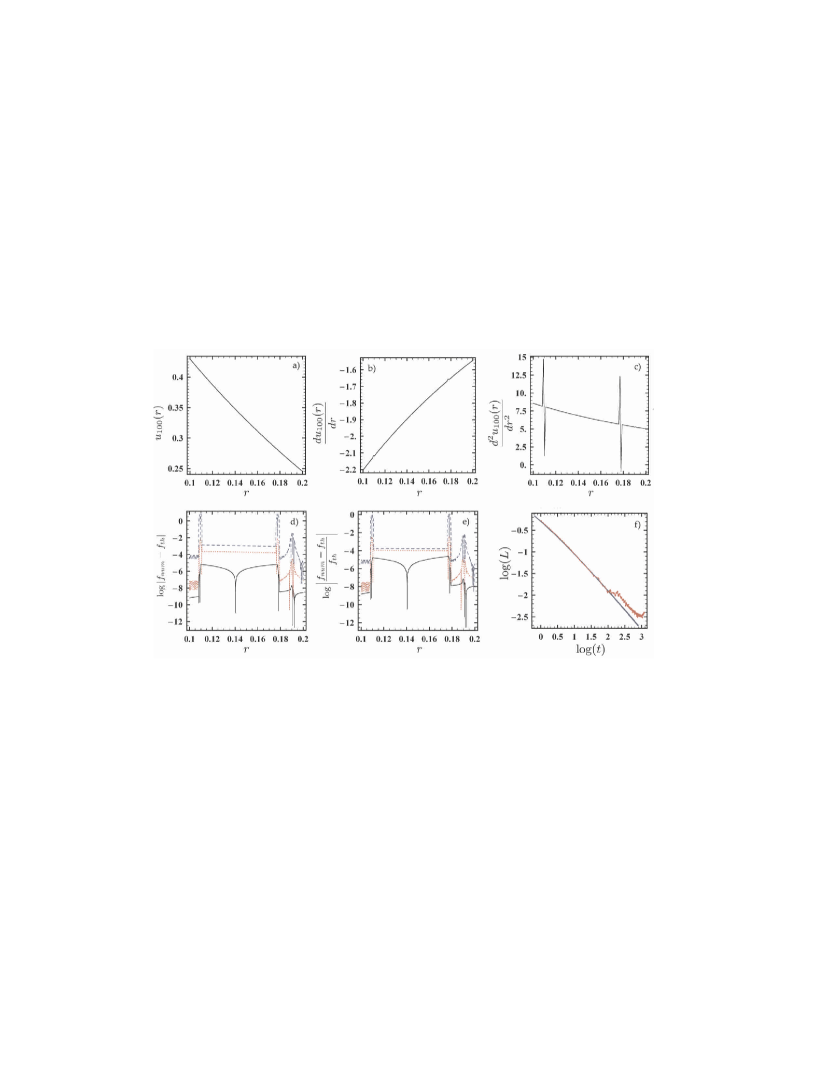
Figure 2: (a) The HO eigenfunction $u_{100}(r)$ $(n=1,l=m=0)$ versus $r$ as derived by the SLEDGE solver of the corresponding Sturm-Liouville problem, after a cubic spline interpolation of the numerical values on a grid of stepsize $dr=0.001$. (b) The derivative of the curve (a) as calculated by the interpolating function. Two non smooth spots are just visible at $r\simeq 0.11$ and $r\simeq 0.175$ respectively. (c) Second derivative of (a). The error at the two spots is now clearly amplified, creating large errors in the variational equations of motion in which the second derivatives of the eigenfunction appear. (d), (e) The absolute and relative errors of the interpolated numerical solution with respect to the analytical solution in logarithmic scale for the function $u_{100}$ (black solid line), and for the derivatives $du_{100}(r)/dr$ (red dotted line) and $d^{2}u(r)_{100}(r)/dr^{2}$ (blue dashed line). The error in the first derivative is amplified with respect to the error in the eigenfunction, while the error in the second derivative becomes of order unity at the spots. (f) The evolution of the finite time Lyapunov characteristic number (LCN) for one orbit in the maximally triaxial Dehnen model with $\gamma=0.4$ (see section 4), initial conditions $x_{0}\simeq 0.045760$, $y_{0}\simeq 0.004794$, $z_{0}\simeq 0.001598$, $v_{x0}=0$, $v_{y0}=0$, $v_{z0}=0$, when the potential is reproduced by the HO basis set calculated analytically (blue solid curve) or numerically (by the SLEDGE code) on a grid (red dashed curve). The expansions in both cases reach up to $n_{max}=9$ and $l_{max}=4$. The LCN curve shows the orbit to be regular in the first case, and chaotic in the second case with $LCN\approx 10^{-2.5}$.

Weinberg (1999) stressed the need for an adaptive algorithm producing basis sets tailored to the morphological details of the system under study, so that the series representation of the potential has good convergence properties and numerical instabilities such as that mentioned in the previous section are avoided. Translated to spherical coordinates, Weinberg’s proposal is essentially the following:

a) Choose kernel functions $\rho_{lm}(r),\Phi_{lm}(r)$ which are as good estimators as possible of the profiles of the $N$-body system to be run.

b) Solve numerically the Sturm-Liouville boundary value problem (6) by special solvers such as the SLEDGE code (Pruess & Fulton 1993). Such solvers are based on variants of the shooting method, and they yield the solutions $u_{nlm}$ in tabulated form, i.e., at the points of a grid.

In principle, Weinberg’s proposal extends considerably the applicability of the SCF method by enlarging the freedom of choice of kernel functions $\Phi_{lm}(r),\rho_{lm}(r)$, which can even be adaptive, i.e., change in the course of an $N$-body simulation. However, we show now that the use of tabulated values on a grid imposes restrictions to accuracy so that we have to devise an alternative method for the solution of the Sturm-Liouville problem.

To this end, we point out first that when the functions $u_{nlm}$ are known only on a grid, the first and second derivatives of the potential can be calculated directly only by a finite difference scheme. However, the use of any such scheme whatsoever cancels the property of smoothness of the potential. In order to retain the latter we can use an interpolating function for each tabulated function $u_{nlm}$, with sufficient number of continuous derivatives, that joins the values of any function $u_{nlm}(r)$ at successive points of the radial grid. However, if there are small numerical errors at the grid points, these errors also show up when one calculates the derivatives either by finite differencing or by the derivatives of the interpolating function. Fig. 2 shows how does the error appear when using interpolation. The SLEDGE solver was used in order to produce numerically the HO basis set $u_{nlm}$, which is given analytically by Eq.(17) with $l=0,\ldots,4$ and $n=0,\ldots,9$, so that comparisons between the numerical and analytical solution can be made. The solution was required on a grid of $2.2\times 10^{4}$ points in the interval $0\leq r\leq 22$, with a tolerance $10^{-8}$. After the basis functions were calculated, each function was interpolated by a cubic spline, so as to secure the continuity of the first and second derivative of the interpolating function at the grid points. Fig. 2a shows the interpolated numerical solution in the case $n=1$ and in the interval $0.1\leq r\leq 0.2$. Although SLEDGE could not reach the requested input tolerance $10^{-8}$ in many parts of the solution, the error actually rendered by SLEDGE in the values of the function $u_{100}$ was still relatively small (of order $10^{-6}$ or below, Fig. 2d,e). However, this small error is amplified when one calculates the derivatives $\dfrac{du_{100}}{dr}$ (Fig. 2b) via the interpolating function. Then the error becomes, in general, of order $10^{-4}$, reaching up to $10^{-2}$ at some particular points of the numerical solution (Fig. 2d,e). In fact, a careful examination of these points showed that the grid solution had small jumps there, of order $10^{-6}$, and these were forcing the interpolating function to introduce artificial points at which the convexity was seriously distorted (a function could even turn locally from convex to concave). Thus, when calculating the second derivative $\dfrac{d^{2}u_{100}}{dr^{2}}$, the error was dramatically amplified at these particular points (Fig. 2c). We see that the error locally becomes of order unity, while the overall error in the second derivatives ranges from $10^{-4}$ to $10^{-2}$, i.e., similarly as for the forces. We found similar numerical effects in practically all the functions $u_{nlm}$ that were determined numerically by the SLEDGE solver. Furthermore, when orbits were calculated in an $N$-body realization of a maximally triaxial Dehnen $\gamma-$model, for $\gamma=0.4$ (see next section), using the HO basis set calculated numerically up to $n_{max}=9$, $l_{max}=4$, we found orbits that were affected by these errors to such an extent that artificial positive Lyapunov characteristic numbers were introduced in cases of orbits that were in fact regular (Fig. 2f).

In order to overcome the above numerical difficulties, we suggest now a ‘quantum-mechanical’ method of solution of the Sturm-Liouville problem (6) which is similar to the quantum-mechanical perturbation theory of bound eigenstates (e.g. Merzbacher, 1961, pp.413-437). This method is applicable when a numerical basis set is required that is not very different from another basis set known analytically . Let $u^{(0)}_{nlm}(r)$ be the functions of the known set. These are solutions of the problem (6) for a Sturm-Liouville operator ${\cal L}^{(0)}_{lm}$, which is determined by a choice of kernel functions as, e.g., in subsection 2.2, and for specific boundary conditions of the form (10). Let, now, ${\cal L}_{lm}$ be a different Sturm-Liouville operator corresponding to a different choice of kernel functions. We seek to solve the eigenfunction problem

$${\cal L}_{lm}u_{lm}(r)=\lambda w_{lm}(r)u_{lm}(r)$$ (20)

i.e., find the spectrum of successive eigenvalues $\lambda_{n^{\prime}}$ and eigenvectors $u_{n^{\prime}lm}(r)$ of ${\cal L}_{lm}$, $n^{\prime}=0,1,...$, for which we request to satisfy the same boundary conditions as those satisfied by the functions $u^{(0)}_{nlm}(r)$. Since the latter form a complete basis of the space of functions with the given boundary conditions, any function can be written as a linear combination of them. We thus write

$$u_{n^{\prime}lm}(r)=\sum_{n=0}^{\infty}d_{n^{\prime},nlm}u^{(0)}_{nlm}(r).$$ (21)

In view of (20), Eq.(21) takes the form

$$\sum_{n=0}^{\infty}d_{n^{\prime},nlm}{\cal L}_{lm}u^{(0)}_{nlm}(r)=\lambda_{n^{\prime}}\sum_{n=0}^{\infty}d_{n^{\prime},nlm}w_{lm}(r)u^{(0)}_{nlm}(r).$$ (22)

Multiplying both sides of (22) with $\dfrac{w^{(0)}_{lm}(r)u^{(0)}_{jlm}(r)}{w_{lm}(r)}$, integrating over all radii from $r_{a}$ to $r_{b}$, and recalling the orthogonality of the functions $u^{(0)}_{nlm}(r)$ yields the linear set of equations:

$$\sum_{n=0}^{\infty}<u^{(0)}_{jlm}|{\cal M}_{lm}|u^{(0)}_{nlm}>d_{n^{\prime},nlm}=\lambda_{n^{\prime}}d_{n^{\prime},jlm}$$ (23)

where the linear operator ${\cal M}_{lm}$ is defined as

$${\cal M}_{lm}={w^{(0)}_{lm}(r)\over w_{lm}(r)}{\cal L}_{lm}$$ (24)

and

$$<u^{(0)}_{jlm}|{\cal M}_{lm}|u^{(0)}_{nlm}>\equiv\int_{r_{a}}^{r_{b}}u^{(0)}_{jlm}(r){\cal M}_{lm}u^{(0)}_{nlm}(r)dr.$$ (25)

The problem (25) is equivalent to the original eigenvalue problem and it can be written in the matrix form:

$${\cal H}_{lm}\cdot{\mathbf{d}_{n^{\prime},lm}}=\lambda{\mathbf{d}_{n^{\prime},lm}}$$ (26)

where ${\mathbf{d}_{n^{\prime},lm}}$ is a column vector with entries equal to the coefficients $d_{n^{\prime}nlm}$, that is ${\mathbf{d}}_{n^{\prime},lm}^{T}=(d_{n^{\prime},0lm},d_{n^{\prime},1lm},d_{n^{\prime},2lm},\ldots)$, and ${\cal H}_{lm}$ is a matrix with entries ${\cal H}_{lm,ij}=<u^{(0)}_{ilm}|{\cal M}_{lm}|u^{(0)}_{jlm}>$. This formally corresponds to what is referred to as the ‘Hamiltonian matrix’ in quantum mechanics, while Eq.(26) is analogous to the quantum mechanical procedure of diagonalization of the Hamiltonian matrix.

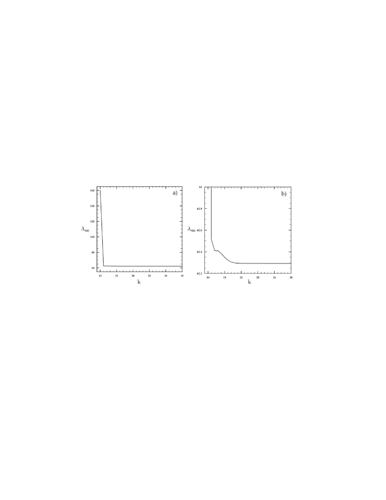
Figure 3: (a) The numerical value of the eigenvalue $\lambda_{900}$ of the new basis set as a function of the rank $k$ (order of truncation of the matrix $\cal H$) when $\varepsilon=0.02$. Note that we need at least a $10\times 10$ matrix in order to start calculating this eigenvalue. (b) A zoom of (a) in which the convergence of the eigenvalue $\lambda_{900}$ to a final value, as $k$ increases, is shown in greater detail. The final value is practically reached when $k\gtrsim 20$.

The numerical steps in order to solve the Sturm-Liouville problem (20) are then summarized as follows:

a) Starting from a known basis set $u^{(0)}_{nlm}$, calculate the integrals (25) and hence the matrix ${\cal H}_{lm}$. In fact, the matrix ${\cal H}_{lm}$ contains an infinite number of entries, thus we can only compute $k\times k$ truncations of ${\cal H}_{lm}$. Nevertheless, the determination of the eigenvalues and eigenvectors of (26) for different truncation orders $k$ is a convergent procedure (numerical examples are given below). The convergence is faster when the set of eigenfunctions $u^{(0)}_{nlm}$ and $u_{nlm}$ correspond to ‘nearby’ operators ${\cal M}_{lm}^{(0)},{\cal M}_{lm}$. By this we mean that the kernel functions $\Phi^{(0)}_{lm}(r),\Phi_{lm}(r)$, and $w^{(0)}_{lm}(r),w_{lm}(r)$, through which the operators ${\cal M}_{lm}^{(0)}$ and ${\cal M}_{lm}$ are defined, should have a small distance in their functional space, the latter being defined for two arbitrary functions $f,g$ as, for example, the euclidian distance

$$d^{2}(f,g)=\int_{r_{a}}^{r_{b}}(f(r)-g(r))^{2}dr.$$ (27)

b) Solve the eigenvalue problem (26) for the $k\times k$ truncated problem. This determines eigenvalues $\lambda_{n^{\prime}lm}$ and eigenvectors ${\mathbf{d}}_{n^{\prime},lm}$. The latter are translated to the new eigenfunctions $u_{n^{\prime}lm}(r)={\mathbf{d}}_{n^{\prime}lm}^{T}\cdot{\mathbf{u}^{(0)}_{lm}(r)}$, where ${\mathbf{u}^{(0)}_{lm}(r)}$ is the column matrix with the functions $u^{(0)}_{nlm}(r),n=0,1,2,\ldots k-1$ as entries. Notice that the matrix ${\cal M}_{lm}$ is real and symmetric, thus its diagonalization is a numerically fast and accurate procedure.

We have implemented the above procedure in order to produce a numerical basis set that satisfies the following two properties:

i) It is ‘nearby’ to the HO basis set in the sense of small functional distance of the kernel functions given by Eq.(27).

ii) It can reproduce density profiles which are shallower in the centre than $\rho(r)\propto r^{-1}$.

The new basis set was defined as follows: Selecting the initial kernel functions $\Phi^{(0)}_{lm}(r),\rho^{(0)}_{lm}(r)$ and basis functions $u^{(0)}_{nlm}$ to be the HO set, we define the new kernel functions

$$\Phi_{lm}(r) =\Phi^{(0)}_{lm}(r)$$ (28a)

$$\rho_{lm}(r) =\sqrt{4\pi}\frac{1}{2\pi}\frac{(2l+1)(l+1)}{(r^{2}+\varepsilon^{2})^{1/2}}\frac{ar^{l}}{(a+r)^{2l+3}}.$$ (28b)

Thus, the only change with respect to the HO set is the introduction of a softening parameter $\varepsilon$ in the singular factor $1/r$ of the HO density kernel function. It follows that the operators ${\cal L}^{(0)}_{lm},{\cal L}_{lm}$ are identical ${\cal L}^{(0)}_{lm}={\cal L}_{lm}$, but the operators ${\cal M}^{(0)}_{lm},{\cal M}_{lm}$ are different, ${\cal M}^{(0)}_{lm}\neq{\cal M}_{lm}$, because $w^{(0)}_{lm}(r)\neq w_{lm}(r)$. Furthermore,

$$\lim_{\varepsilon\rightarrow 0}d(w^{(0)}_{lm},w_{lm})=0$$

thus, for $\varepsilon$ sufficiently small, the operators ${\cal M}^{(0)}_{lm},{\cal M}_{lm}$ are ‘nearby’ according to the previously given definition.

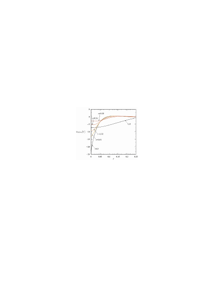
Figure 4: The forms of the radial basis functions $u_{52m}(r)$ ($n=5$, $l=2$, independent of $m$) in the inner region ($r<0.25$) in the HO and CB cases and in the case of the ‘quantum-mechanical’ calculation for various values of the parameter $\varepsilon$.

Fig. 3 shows the convergence of the numerical solution of the eigenvalue problem (26) for the above kernel functions, as a function of the truncation order $k$. The abscissa in Fig. 3a,b is the dimension $k$ of the $k\times k$ matrix ${\cal H}_{lm}^{\mbox{k-th truncation}}$ . The ordinate shows the numerical value $\lambda_{900}$ (in the case $\varepsilon=0.02$) of the eigenvalue of the tenth eigenvector of ${\cal H}_{lm}^{\mbox{k-th truncation}}$ which corresponds to the quantum numbers $n=9$, and $l=m=0$. Clearly, when $k$ is as small as $k=11$, the numerical value of $\lambda_{900}$ calculated from the matrix ${\cal H}_{00}^{\mbox{k-th truncation}}$ is already very close to the value $\lambda_{900}\simeq 62.29235$ corresponding to the limit $k\rightarrow\infty$. A zoom of Fig. 3a is shown in Fig. 3b, in which we see that the limiting value of $\lambda_{900}$ is practically reached after $k\gtrsim 20$. In fact, we always find that the limiting values of the eigenvalues from $\lambda_{0lm}$ up to $\lambda_{nlm}$ are specified essentially up to the computer’s double precision limit when one uses matrices ${\cal H}_{lm}$ truncated at an order $k=3n$.

Fig. 4 shows an example of numerical basis function ($u_{52m}(r)$ for $n=5$, $l=2$, independent of $m$) calculated for different values of the parameter $\varepsilon$, compared to the HO and CB basis functions for the same quantum numbers. The plot focuses on the region of inner radii ($r\leq 0.25$). Clearly, when $r>0.15$ all the numerical basis functions are much closer to the HO basis set than to the CB basis set, while, at radii below $r=0.15$ the effect of introducing $\varepsilon$ is manifested, namely a basis function becomes less steep at the centre as the value of $\varepsilon$ increases. Thus, by choosing different values of $\varepsilon$ we can better control different behaviors of the central potential or density profiles of a simulated system. We also note that the CB basis function deviates considerably at the centre from both the HO and the numerical basis functions, a fact expected since the CB kernel function (Plummer sphere) represents systems which are rather flat at the centre.

4 A Numerical Test. The degree of order and chaos via the SCF method

In the present section our task is to test the accuracy of reproduction of the orbital content of a model elliptical galaxy by various SCF codes differing in the choice of radial basis set. The model is Denhen’s (1993) $\gamma-$model with an ellipsoidal radius $m$ (Merritt 1999, section 1). The density reads:

$$\rho_{\gamma}(m)=\frac{(3-\gamma)r_{a}M}{4\pi abc}m^{-\gamma}(r_{a}+m)^{-(4-\gamma)}$$ (29)

with $0\leq\gamma<3$, where

$$m^{2}={x^{2}\over a^{2}}+{y^{2}\over b^{2}}+{z^{2}\over c^{2}}$$ (30)

is the ellipsoidal radius corresponding to a triaxial system with axial ratios $a:b:c$, $a\geq b\geq c>0$, and $M$ equal to the total mass of the galaxy. The parameter $\gamma$ determines the exponent of the power-law profile of the density at the centre, i.e., $\rho(m)\sim m^{-\gamma}$ at the centre which essentially yields also a radial profile $\rho(r)\sim r^{-\gamma}$. We are interested in the case of ‘core’ galaxies in which $\gamma$ is in the range $0\leq\gamma\leq 1$. The potential corresponding to the density (29) reads (Merritt & Fridman 1996):

$$\Phi(x,y,z)=-\frac{M}{2(2-\gamma)r_{a}}\times\int_{0}^{\infty}\tfrac{1-(3-\gamma)\left(\tfrac{m^{\prime}}{r_{a}+m^{\prime}}\right)^{2-\gamma}+(2-\gamma)\left(\tfrac{m^{\prime}}{r_{a}+m^{\prime}}\right)^{3-\gamma}}{\sqrt{(\tau+a^{2})(\tau+b^{2})(\tau+c^{2})}}d\tau$$ (31)

with

$$m^{\prime 2}={x^{2}\over a^{2}+\tau}+{y^{2}\over b^{2}+\tau}+{z^{2}\over c^{2}+\tau}.$$

Figure 5: (a) The $x$ axis component $F_{x}$ of the force along the direction $x=y=z=r$ for the Dehnen model $\gamma=0.4$ (black solid line) and the approximations of the same force component obtained by implementing the SCF method to the $N$-body realization of the Dehnen model using the HO, CB and the $\varepsilon$-modified basis sets (the values of $\varepsilon$ are indicated in the figure. The number of particles in the $N$-body realization are $1.25\times 10^{7}$. (b) a focus of (a) near the centre. The force with HO has a finite value at $r=0$, while the force with CB is zero at the centre but its overall central profile is much smoother than in reality. On the other hand, all the $\varepsilon$-modified basis sets behave better than the HO or CB sets at the centre. The optimal value of $\varepsilon$ by visual inspection is close to $\varepsilon=0.02$.

In order to produce an $N$-body realization of the previous system, we work as in the numerical example of subsection (2.2) using $N=1.25\times 10^{7}$ particles arranged in a $(50\times 100\times 200)$, spherical polar grid. We found that such a number of particles was necessary because the results regarding all the tests below were becoming robust against the number of particles for $N$ of the order of $N=10^{7}$ or higher. This fact is related to various effects caused by the Poisson noise (subsection 4.2 below). The unit of length is determined so that the half-mass radius is at $r_{1/2}=1$, while the $N$-body system is truncated at a radius $r=15$, containing 95% of the total mass of the model system (in which the distribution of the mass extends theoretically to the limit $r\rightarrow\infty$).

In all the models we set $a=1$, $b=0.7905$, $c=0.5$ corresponding to a maximally triaxial model. Six different Dehnen models of progressively higher power-law exponents were examined, namely $\gamma=0$ (perfectly harmonic core), $\gamma=0.2$, $0.4$, $0.6$, $0.8$, and $1$ (weak cusp). After the $N$-body realization for each of these models was produced, the potential and density were fitted by the SCF method using eight different radial basis sets. These are the HO and the CB sets, as well as the basis sets derived by the ‘quantum-mechanical’ method of section 3, for the values of the parameter $\varepsilon$ equal to $\varepsilon=0.005$, $0.01$, $0.02$, $0.04$, $0.06$ and $0.08$. The latter are called $\varepsilon-$modified basis sets (modified with respect to the HO basis set).

There are two different numerical tests performed in these systems: a) we compare the accuracy of reproduction of the behavior of the forces of the Dehnen model at the centre, for each choice of SCF basis set, and b) we compute a library of 1200 orbits and compare the number of orbits that are found to be regular or chaotic, as well as the distribution of the Lyapunov characteristic numbers produced by the numerical integration of the variational equations of motion in each potential representation. In the sequel we separately analyze these two categories of numerical tests and compare their outcome as regards the ‘optimal’ basis set to be used, i.e., the value of $\varepsilon$ for which the Dehnen model and SCF agreement are better. This information is given as a function of the value of $\gamma$.

Figure 6: The quantity $\frac{1}{3}\sum\limits_{a=(x,y,z)}\frac{\overline{\Delta F_{a}^{2}}}{F_{ch}^{2}}$ versus $\varepsilon$ for each $\gamma-$model examined. The quantity $\overline{\Delta F_{a}^{2}}$ is the mean square difference, inside a central sphere of radius $r=0.01$, between the force component $a$ (where $a$ can be $x,y,z$) of the specific $\gamma-$model and the same force component as derived from different SCF basis sets implemented to the $N$-body realization of the Dehnen model. The quantity $\overline{F}_{ch}$ is a characteristic value of the force for all the models set equal to $\overline{F}_{ch}=10^{7}$. The red and the blue horizontal lines correspond to the HO and CB basis sets, respectively. (a) $\gamma=0$, (b) $\gamma=0.2$, (c) $\gamma=0.4$, (d) $\gamma=0.6$, (e) $\gamma=0.8$, (f) $\gamma=1$. For $\gamma=0$ the minimum error is for $\varepsilon=0.04$. As $\gamma$ increases the optimal value of $\varepsilon$ decreases. After $\gamma=0.8$, the HO basis set gives smaller error than the $\varepsilon-$modified basis sets, which, however, remains in relatively higher levels than the minimum error found for smaller values of $\gamma$. The CB basis set gives the worst results (as regards the force error) for all the values of $\gamma$.

4.1 Forces

Fig. 5 shows the reproduction of the forces by the eight different SCF basis sets in the $N$-body realization of the $\gamma=0.4$ model, compared to the analytically derived forces through the differentiation of (31) with respect to the coordinate variables. In all calculations below the ten first radial basis functions $n=0,1,\ldots 9$ are used for each angular function $Y_{l}^{m}$, with $l=0,\ldots 4$, $m=-l,\ldots,l$. We found that despite the large increase in the number of basis functions there was practically no significant difference observed when $n$ was raised up to $n_{max}=13$ and $l$ up to $l_{max}=6$. The odd angular functions $l=1,3$ or $m=1,3$ are kept in the SCF calculation despite the fact that theoretically the coefficients of the corresponding terms in the potential or density expansion are zero (because the Dehnen model is fully symmetric with respect to the three principal planes $(x-y)$, $(x-z)$, or $(y-z)$). Numerically, these coefficients turn to have small values that yield an estimate of the effect of the Poisson noise of the $N$-body realization on the numerical values of the coefficients. In Fig. 5, The $F_{x}$ projection of the force is plotted as a function of $r$ when the force is calculated in the direction $x=y=z=r$. Fig. 5a refers to a radial extent up to $r=1$, i.e., up to the half-mass radius of the system. We see that all the SCF models provide in general a satisfactory reproduction of the true force in this range, except for the CB model for which the agreement is good only in the outer radii ($r>0.2$). On the other hand, the various models are diversified in their behavior close to the centre, which is seen by zooming to $0\leq r\leq 0.1$ in Fig. 5b. We notice immediately the failure of both the HO and CB sets to provide a reasonable representation of the forces in this scale. The force, as derived by the HO set, turns to have a significantly non-zero value at the centre. This is precisely the problem of the non-perfect balancing of the coefficients analyzed in subsection (2.2). On the other hand, the CB set yields a zero force at the centre, but near the centre the force is seriously softened with respect to the true force. One obtains a better agreement if one uses the $\varepsilon-$modified basis sets, as exemplified by the plots of Fig. 5b for $\varepsilon=0.01$, $0.02$, or $0.06$.

In order to quantify the quality of the fit of the forces by the different SCF models, we cannot use as a relevant quantity the fractional errors $\Delta F(r)/F(r)$, as a function of $r$, because we have $F(r)\rightarrow 0$ as $r\rightarrow 0$, yielding fractional errors $\Delta F(r)/F(r)\rightarrow\infty$ in this limit. We thus use as a relevant index the quantity

$$<{\Delta F^{2}\over F^{2}}>={1\over 3}\sum_{\alpha=x,y,z}^{3}{\overline{\Delta F_{\alpha}^{2}}\over\overline{F}_{ch}^{2}}$$ (32)

where $\overline{\Delta F_{\alpha}^{2}}$ is the average value of the squared differences of the forces in the axis $\alpha=x,y,z$ in a spherical volume $0\leq r\leq 0.01$ and $\overline{F}_{ch}$ is a characteristic value of the force set equal to $\overline{F}_{ch}=10^{7}$, used to normalize the errors of all the models. The quantity $<{\Delta F^{2}\over F^{2}}>$ for the eight SCF models, and for all the different $\gamma-$models is shown in Fig. 6 (the case $\gamma=0.4$ of Fig. 5 corresponds to the panel 6c). In the ideal ‘harmonic core’ case (Fig. 6a, $\gamma=0$), a significantly non-zero value of $\varepsilon$ ($\varepsilon_{optimal}\simeq 0.04$) is required in order to minimize the error in the central forces to a level $<{\Delta F^{2}\over F^{2}}>\sim 10^{-3}$. On the other hand, as $\gamma$ increases, the optimal value $\varepsilon_{optimal}$, at which the force error is minimized, is shifted towards smaller values of $\varepsilon$ ($\varepsilon_{optimal}\simeq 0.02$ when $\gamma=0.2$ (Fig. 6b), $\varepsilon_{optimal}\simeq 0.01$ when $\gamma=0.4$ (Fig. 6c), $\varepsilon_{optimal}\simeq 0.005$ when $\gamma=0.6$ (Fig. 6d)). When $\gamma=1$, the $\varepsilon-$modified basis set yields worse results than the HO basis set, while it is still better than the CB set (Fig. 6e,f). A typical estimate of force errors with the HO basis set is $<{\Delta F^{2}\over F^{2}}>\sim 10^{-1}$. We emphasize that such errors in the force determination appear inside a very small region of the galaxy (up to $r=0.01$ when the half-mass radius is $r=1$). Thus, one may claim that the errors are not important in the overall $N$-body simulation. Nevertheless, these errors are important when one calculates the regular or chaotic character of the orbits, as demonstrated in the next subsection.

4.2 Lyapunov exponents and the regular or chaotic character of the orbits

In order to check numerically the regular or chaotic character of the orbits, we create, for each $\gamma-$model, a library of 1200 orbits calculated by a set of initial conditions uniformly distributed on four different equipotential surfaces of the $\gamma-$model potential $\Phi_{\gamma}(x,y,z)$ corresponding to the values of the energy $E_{1}=0.95\Phi_{\gamma}(0,0,0)$, $E_{2}=0.8\Phi_{\gamma}(0,0,0)$, $E_{3}=0.6\Phi_{\gamma}(0,0,0)$ and $E_{4}=0.4\Phi_{\gamma}(0,0,0)$. In the energies $E_{1}$ and $E_{2}$, which are close to the central value of the potential, we find many ‘box’ orbits which are regular. The existence of box orbits is actually guaranteed by the fact that the force at the centre is zero for $\gamma<1$. On the other hand, as the value of the energy increases the phase space is dominated by different families of tube orbits or chaotic orbits. The tube orbits follow essentially the classification of Statler (1987) for the perfect ellipsoid. In general, chaos increases as the value of $\gamma$ increases, a fact mainly associated with the destruction of the regular character of the box orbits.

Figure 7: The method used to distinguish between regular and chaotic orbits. The Alignment Index $AI_{j}$, $j=1,...,1200$ of each orbit is plotted against the finite time Lyapunov number $L_{j}$ in $\log-\log$ scale. A detailed description of this method is given in Voglis et al. (2002). The specific plot refers to the case of Dehnen model with $\gamma=0.6$. Each point in this plot corresponds to an orbit that was integrated for $1200$ radial periods. Regular orbits have low values of $L_{j}$ (decreasing with the integration time as $t^{-1}$) and high values of $AI_{j}$, thus the group of regular lies in a region near $\log(L_{j})\approx-3$ and $\log(AI_{j})\gtrsim-3.5$. Chaotic orbits have large values of $L_{j}$ and very small values of $AI_{j}$ ($AI_{j}<10^{-10}$). The orbits on a lane joining the above two groups are weakly chaotic orbits (i.e. sticky orbits) which have just started exhibiting their asymptotic chaotic behavior.

Figure 8: The distribution of the values of $\log(L)$ of the chaotic orbits for the Dehnen model $\gamma=0.6$ (same black solid line in each panel) compared to those found by the HO, the $\varepsilon-$modified (for the indicated values of $\varepsilon$) and the CB basis sets (blue dashed lines) in the $N$-body realization of the same system. From these figures it is clear that HO overestimates chaos, CB underestimates chaos and the best estimation is obtained by an $\varepsilon-$modified basis set for $\varepsilon$ between $\varepsilon=0.005$ and $\varepsilon=0.01$. Odd angular terms $l,m=1,3$ are excluded from the computation because they are affected by Poisson-noise asymmetries in the $N$-body realization (see text for details).

Figure 9: The percentages of chaotic orbits in the original Dehnen models and with the various SCF basis sets applied to the corresponding $N$-body realizations. Each panel indicates the corresponding value of $\gamma$. Black solid lines correspond to the percentages of chaotic orbits in the original Dehnen models, pale blue (dotted) and blue (dashed) lines to the calculation with CB, with and without odd angular terms, orange (dotted-dashed) and red (dashed) lines to the calculation with HO, with and without the odd angular terms. Black solid curves correspond to the calculation with the $\varepsilon-$modified basis sets for the various values of $\varepsilon$ (curves with open circles = calculation with the full angular expansion, curves with solid rectangles = calculation without odd angular terms). The optimal value of $\varepsilon$ with respect to the criterion of agreement in the percentage of chaos is determined by the point where the curve of the $\varepsilon-$modified calculations (curve with solid rectangles) intersects the horizontal black line (original Dehnen model)

.

In order to characterize the orbits as regular or chaotic we use the same numerical criterion as in Voglis et al. (2002). This is a combination of two numerical indices, called the ‘finite-time-Lyapunov number’ $L_{j}$ and the ‘Alignment index’ $AI_{j}$ respectively (see Voglis et al. 2002 for details). The numerical values of these indices are calculated for each orbit, labelled by the index $j$, over an integration time equal to $T=1200$ radial periods. In a two-dimensional plot of $\log(AI_{j})$ versus $\log(L_{j})$ (Fig. 7, for $\gamma=0.6$), the regular orbits accumulate in the right and middle part of the diagram, in an almost straight horizontal segment around the value $\log(L_{j})\simeq\log(1/T)\simeq-3$. On the contrary, the chaotic orbits occupy the up and left part of the diagram and have a considerable scatter in the values of $L_{j}$, which are a measure of the maximal Lyapunov characteristic exponent of the orbits. In between these two groups of points there is a lane of points connecting the two groups. This refers to weakly chaotic, or ‘sticky’ orbits, and as $T$ increases, there is a continuous, albeit decreasing, flow of points through the lane towards the group of chaotic orbits. However, this flow is irrelevant in the characterization of the orbits for times greater than $T$, because it should imply that some orbits characterized as ‘chaotic’ have, in fact, Lyapunov times much longer than the age of the galaxy.

Fig. 8 shows, now, the main result as regards the choice of an appropriate set of basis functions that better reproduces the regular or chaotic character of the orbits. All the panels show the distributions of the logarithm of the finite-time Lyapunov numbers $L_{j}$ in the case $\gamma=0.6$ for the orbits which are within or above the transport lane of Fig. 7, i.e., the orbits characterized as chaotic. The distributions are not normalized, i.e., the area below each distribution is equal to the percentage of orbits that were characterized as chaotic. Thus, differences in the total area covered by two distributions mean a difference in the total percentage of the orbits characterized as chaotic, while differences in the shape reflect a different normalized distribution of Lyapunov exponents. The distribution shown with solid line refers to the precise calculation in the analytic Dehnen force field, while dashed plots refer to computations with different SCF basis sets. Furthermore, in this figure all the SCF distributions refer to a calculation in which we switched off the odd terms of the angular expansion of the potential as derived by the SCF code for reasons explained immediately below.

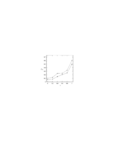
Figure 10: The percentages of chaotic orbits found by the use of the optimal basis set (see Fig. 9), for each value of $\gamma$, when the non-symmetric (odd) angular terms in the potential expansion are turned on (lower curve) or off (upper curve).

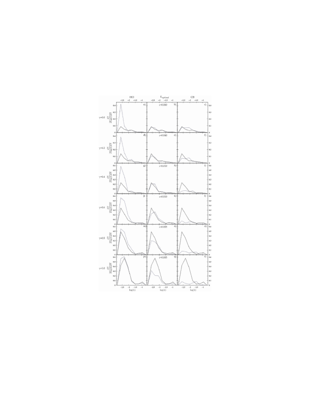
Figure 11: The $\log(L)$ distributions of the chaotic orbits as derived by the HO, optimal $\varepsilon-$modified, and CB approximations compared to the true distribution of the corresponding Dehnen model. Each row refers to one indicated value of $\gamma$. Black solid curves correspond to the real distribution while blue dashed curves are the distributions with HO (left column), optimal $\varepsilon-$modified (middle column), or CB (right column) we have for the specific value of $\gamma$. For $\gamma\leq 0.6$ the agreement is better between the real and optimal $\varepsilon-$modified calculations. For $\gamma=0.8$ the results with $\varepsilon-$modified ($\varepsilon=0.005$) and HO ($\varepsilon=0$) are comparable, while for $\gamma=1.0$ the best result is with HO.

The following are some basic remarks regarding these diagrams:

a) The computation with the HO basis set overestimates by a factor of about 1.7 the percentage of chaotic orbits in this model. Thus, as shown below, while the true percentage for $\gamma=0.6$ is $\simeq 22\%$, the HO fit yields $\simeq 38\%$. In fact, the difference in the two percentages is even higher if one takes into account the odd terms of the angular expansion of the potential (in this case we find a percentage $48\%$ with the HO basis set). However, we know that the true value of these terms in the Dehnen model is equal to zero, so that non-zero values can only be associated with asymmetries in the number of particles on the two sides of any of the principal planes of the galaxy induced by the Poisson noise of the $N$-body realization. The simplest way to measure the latter is by measuring the size of the coefficients of the odd angular functions $l=1,3$ or $m=1,3$ in the potential expansion. We thus use the following measure of the Poisson noise:

$$PN={||\mbox{coefficients of odd angular terms}||\over||\mbox{all coefficients}||}$$ (33)

where the norm $||\cdot||$ means sum of the absolute values of the coefficients. In the case of Fig. 8a, we find $PN\simeq 2.3\times 10^{-3}$ which is consistent with an estimate $PN\sim O(1/\sqrt{N})$ with $N=1.25\times 10^{7}$. This looks like a relatively small number, which however produced a 10% difference in the percentage of chaos with the HO simulation.

b) The computation with the CB set (Fig. 8h) underestimates the percentage of chaotic orbits by a factor $\simeq 2.75$ (22% true percentage against 8% with CB). The underestimate is even more serious (6%) if one switches off the odd angular terms. The forms of the two distributions are also quite different, a fact meaning that the CB fit is rather unsuitable to represent a galaxy with central power-law exponent $\gamma=0.6$ (or beyond).

c) The best results are found when we use an $\varepsilon-$modified basis set with $\varepsilon_{optimal}$ between the values $\varepsilon_{optimal}=0.005$ and $\varepsilon_{optimal}=0.01$ (Fig. 8b,c). For this value of $\varepsilon$ both the percentage of chaotic orbits and the distribution of the Lyapunov exponents derived by the SCF method are in good agreement with the true percentage and distribution.

Fig. 9 shows a comparison of the true percentages of chaotic orbits with those found by the SCF fit with different basis sets, for all the examined values of $\gamma$. An optimal value of $\varepsilon$, based on the ‘percentage of chaos’ criterion, is determined by the point where the curves with open dots intersect the horizontal solid line, marking the true percentage. This value, however, is also contaminated by chaos due to the Poisson noise on the odd angular terms, and a better determination is made when these terms are switched off (solid curves with black rectangles). In any case, Fig. 9 renders immediately clear that the HO fit produces overestimates of the percentage of chaotic orbits in the whole range of values $0\leq\gamma\leq 1$, while the CB fit underestimates the percentage of chaos for the values $0.4\leq\gamma$. Up to $\gamma=0.8$ an optimal $\varepsilon-$modified model can be found yielding the best agreement with the true percentage. Near this value of $\gamma$, however, the situation is reversed, and in the limit $\gamma\rightarrow 1$ it is the $\varepsilon-$modified models yielding underestimates and the HO model yielding the best results. This is, precisely what is expected by noticing the $r^{-1}$ power-law profile of the HO monopole terms at the centre.

Fig. 10 shows the comparison of the percentages of chaotic orbits found by the use of the optimal basis set, for each value of $\gamma$, when the non-symmetric (odd) angular terms in the potential expansion are turned on or off. In all cases, the numerical noise due to the non-symmetric (odd) terms increases the percentage of chaotic orbits. This fact justifies the use of symmetrized N-Body realizations of a system, as e.g. by Holley-Bockelmann et al. (2001), when an orbital analysis is requested.

Fig. 11 shows a comparison of the distributions of the finite-time Lyapunov exponents of the chaotic orbits for all the $\gamma-$models considered, with the distributions derived via the HO model, optimal $\varepsilon-$modified, and CB model. This figure checks essentially whether, at the value of $\varepsilon$ at which the agreement of the percentages of chaotic orbits is good, the agreement of the distributions of the finite time Lyapunov numbers is also good. This check is necessary, because it is possible that two very different distributions yet cover the same total area. The plots in the middle column of Fig. 11 clearly show that the distributions with the $\varepsilon-$modified basis set, at the optimal value $\varepsilon=\varepsilon_{optimal}$, are indeed in good agreement with the true distributions, except in the case $\gamma=1$ in which the best agreement is obtained by the HO basis set.

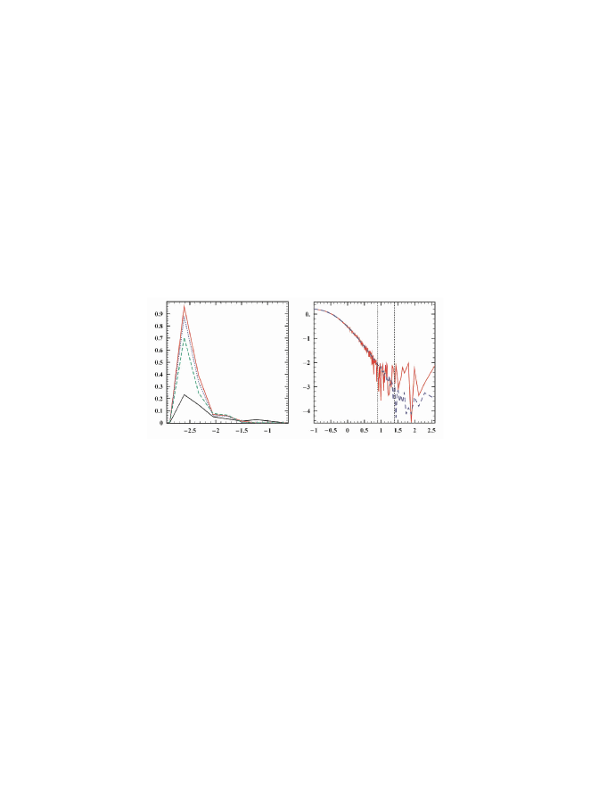
Figure 12: (a) The $\log(L)$ distributions of the chaotic orbits, as derived by the HO basis set (with all terms), in a rejection-acceptance Monte Carlo realization of the $\gamma=0.4$ Dehnen model, when the truncation radius is $r_{t}=15$ (red solid line), $r_{t}=30$ (blue dotted line), $r_{t}=100$ (green dashed line). The real distribution by the original $\gamma$-model is plotted by black solid line. (b) The absolute error $|I(r_{t})-I(\infty)|$ versus $r_{t}$ in $\log-\log$ scale. The red solid line corresponds to evaluations of $I(r_{t})$ using Monte Carlo realizations with $N=10^{5}$ particles while the blue dashed line to Monte Carlo realizations with $N=10^{7}$ particles. We see that beyond a value of $r_{t}$ the error due to Poisson noise dominates the error due to finite radius $r_{t}$.

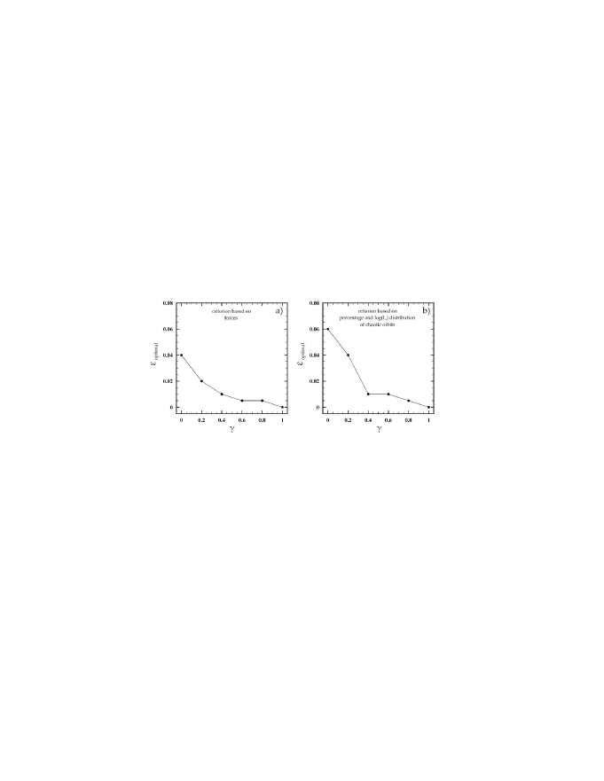
Figure 13: (a) The optimal value of $\varepsilon$ versus $\gamma$ based on the ‘forces’ criterion (see Fig. 6). (b) the optimal value of $\varepsilon$ versus $\gamma$ based on the criterion of the percentage and $\log(L)$ distribution of the chaotic orbits (see Figs. 9 and 10).

In order to check the robustness of the above results on the particular way chosen to create the N-Body realization of a Dehnen $\gamma-$model, we created a different realization, in which there is no use of polar grid, but an acceptance-rejection Monte Carlo algorithm was utilized to produce an N-Body system for the $\gamma=0.4$ model. The mass contained in a small volume element corresponding to values of the spatial coordinates in the intervals $(m,m+dm)$, $(\theta,\theta+d\theta)$, and $(\phi,\phi+d\phi)$ is given by $dm=m^{2}abc\rho(m)\sin(\theta)dm~{}d\theta~{}d\phi$, implying that the mass distribution is separable and uniform in the coordinates $X_{1}=m^{3}/3$, $X_{2}=-\cos(\theta)$ and $X_{3}=\phi$. We thus readily obtain acceptance-rejection Monte Carlo realizations of the models. In practice we transform $m$ to $\xi=(m-1)/(m+1)$ so that when $\xi$ is given values in $-1\leq\xi<1$, $m$ can take arbitrarily large values. In reality, given the finite number of particles in the simulation, the distribution of the matter is undersampled at large radii. We thus checked the robustness of our results against three different truncation radii, namely a) $r_{t}=15$ (which is the standard choice in the previous simulations), b) $r_{t}=30$, and c) $r_{t}=100$. The results are summarized in Fig. 12a, for the distributions of the finite-time Lyapunov numbers calculated with the HO basis set. When the truncation radius is at $r_{t}=30$, there is a marginal improvement of the results (the total percentage of chaotic orbits found is 37%, against 41% when $r_{t}=15$, and 14% real percentage). But even with a much higher truncation radius ($r_{t}=100$) the improvement is still small (32% against 14% real percentage of chaotic orbits). We thus conclude that the distributions shown in Fig. 11 do not change appreciably by changing the sampling technique or the truncation radius.

A simple argument can show why the scaling of the numerical error with the truncation radius $r_{t}$ saturates at some value of $r_{t}$. This is based on equating the error in the evaluation of generalized integrals, due to a truncation of the limits of integration, with the error due to the Poisson noise at large radii by a Monte Carlo evaluation of the integral. Namely, since the Monte Carlo sampling uses a finite number of particles, the drop of the density at large radii implies that the mass distribution is seriously undersampled at these radii. An example is given in Fig. 12b, which refers to a calculation of the integral

$$I(r_{t})=\int_{0}^{r_{t}}4\pi r^{2}\rho(r)\Phi_{00}(r)dr,$$ (34)

corresponding essentially to a truncation at finite radius of the generalized integral (11) for a spherical Dehnen-model $\rho(r)=r^{-\gamma}(1+r)^{-(4-\gamma)}$ when the oscillatory behavior of the functions $u_{n00}(r)$ is neglected. The integral (34) was evaluated by a Monte Carlo sum using $N=10^{5}$ or $N=10^{7}$ particles. Fig. 12b shows the absolute error $|I(r_{t})-I(\infty)|$ when a different Monte Carlo realization of the system is produced for each value of $r_{t}$. For small $r_{t}$, the error is large and it is due to the truncation of the generalized integral at insufficiently small radius. However, beyond a value of $r_{t}$, the Poisson noise due to the undersampling of the density at the outer parts clearly dominates, causing variations of the error which are of the same order as the error due to the finite truncation. When $N=10^{5}$, the critical value of $r_{t}$ is estimated as $r_{t}=8$ (in units of the half-mass radius), and the error beyond this radius fluctuates between $10^{-2}$ and $10^{-3}$. On the other hand, for $N=10^{7}$, the truncation radius beyond which the Poisson noise dominates raises to $r_{t}=25$, and the error beyond this radius fluctuates between $10^{-4}$ and $10^{-3}$. These values are compatible with the estimates given independently in section 2.

Finally, Fig. 13 shows a comparison of the optimal value of $\varepsilon$ determined in the previous analysis by (a) the central force criterion (subsection 3.1), and (b) the chaotic percentage criterion (present subsection). The latter criterion suggests the use of somewhat larger values of $\varepsilon$ than by the former criterion, when $\gamma<0.4$, while the two criteria yield nearly equal values for $\gamma\geq 0.4$. At any rate, the main conclusion drawn from the above numerical examples is that the characterization of the regular or chaotic character of the orbits of an $N$-body system depends crucially on the accurate numerical representation of the ‘smooth’ potential that presumably underlies the mass distribution of the $N$ particles. In the framework of the SCF method, this conclusion is translated into the need for very careful choice of basis set. In the above examples we used a ‘quantum-mechanical’ method in order to calculate numerical basis sets which are close to the HO basis set, but they can better fit the behavior of all smooth quantities (potential, forces, density) at the centre when the power-law central density profile is shallower than $r^{-1}$. Such profiles naturally arise in $N$-body simulations of the remnants of galaxy mergers (e.g. Jesseit et al. 2005 and references there in). Nevertheless, the method is applicable, with different starting basis sets, to a much wider class of stellar dynamical systems and the cautions raised in the present section are, very probably, relevant to such systems as well.

5 Conclusions

In the present paper we address the question of the choice of an optimal basis set of functions for orbital studies of galaxies simulated via the self-consistent field (SCF) method. Our approach is to create $N$-body realizations of a Dehnen analytical $\gamma-$model of a triaxial galaxy and then reproduce the gravitational potential by the SCF method, using different basis sets which are either analytical. i.e., the Hernquist-Ostriker and Clutton-Brock sets, or numerical, depending on a parameter $\varepsilon$ that modifies the behavior of the potential at the centre with respect to the HO basis set. We then compare a number of quantities characterizing the orbits (central force profiles, percentage of chaotic versus regular orbits and distributions of the Lyapunov characteristic numbers) in the original model and in the SCF reproduction of the potential. Our main conclusions are the following:

1) If the kernel functions (section 2) used in the construction of a radial basis set have a singular behavior at the centre, this basis set is unsuitable for simulating galaxies which do not exhibit the same singular behavior. In particular, even if the singularity can be theoretically removed by a balancing of the coefficients of some terms in the SCF series, the numerical noise induced by the Monte-Carlo evaluation of the values of the coefficients destroys the balance and results in large errors appearing in the evaluation of the forces or derivatives of the forces, especially in the central parts of the galaxy.

2) When following the methodology suggested by Weinberg (1999) for the determination of numerical radial basis sets, shooting methods yielding tabulated values of the basis functions on a grid should be avoided, because they, too, introduce large errors in the evaluation of the derivatives of the forces, yielding large inaccuracies in the integration of the variational equations of motion.

3) We propose a ‘quantum-mechanical’ method of determination of numerical radial basis sets that overcomes the above problems. This method is based on the diagonalization of a truncated matrix which results from a spectral formulation of the Sturm-Liouville problem, equivalent to the procedure referred to in quantum mechanics as the diagonalization of the Hamiltonian matrix. The stability and accuracy of this scheme is demonstrated by specific numerical examples.

4) We study the orbits in a family of triaxial Dehnen $\gamma-$models for various values of $\gamma$ in the range $0\leq\gamma\leq 1$, corresponding to the case of elliptical galaxies with ‘shallow’ central cusps. For each $\gamma-$model we use a family of different radial basis functions which are modifications of the HO basis set, derived by implementing the ‘quantum-mechanical’ algorithm of (3). The basis functions depend on one small parameter $\varepsilon$ defined so as to yield the HO basis set in the limit $\varepsilon\rightarrow 0$. The numerical tests concern comparisons of a) the behavior of forces in the central parts of the galaxy, b) the percentage of regular and chaotic orbits, and c) the distribution of the Lyapunov exponents of the chaotic orbits, between the exact $\gamma-$model and the various $N$-body - SCF realizations using the HO, CB and $\varepsilon-$modified models for various values of $\varepsilon$. When the standard basis sets (HO or CB) are used, we find large deviations in all three criteria between the exact and SCF results, except for the HO basis set for $\gamma=1$. On the other hand, the best agreement is found by using $\varepsilon-$modified basis sets for values of $\varepsilon$ in the range $0.005\leq\varepsilon\leq 0.06$ (in units of the half mass radius). The optimal value of $\varepsilon$ is given as a function of the value of $\gamma$. The latter can in principle be determined in advance (before or during the $N$-body simulation) by measuring the power-law exponent of the central radial profile of the system.

All the numerical codes used in the present paper are available by the authors upon request.

References

- Allen et al. (1990) Allen A., Palmer P., Papaloizou J., 1990, MNRAS, 242, 576
- Aoki & Iye (1978) Aoki S., Iye M., 1978, Publ. Astron. Soc. Japan, 30, 519
- Athanassoula (2002) Athanassoula E., 2002, ApJ, 569, L83
- Binney & Tremaine (1987) Binney J., Tremaine S., 1987, Galactic Dynamics. Princeton University Press, New Jersey
- Carpintero & Wachlin (2006) Carpintero D. D., Wachlin F. C., 2006, Cel. Mech. Dyn. Astron., 96, 129
- Clutton-Brock (1972) Clutton-Brock M., 1972, Astroph. & Sp. Sc., 16, 101
- Clutton-Brock (1973) Clutton-Brock M., 1973, Astroph. & Sp. Sc., 23, 55
- Contopoulos et al. (2000) Contopoulos G., Efthymiopoulos C., Voglis N., 2000, Cel. Mech. Dyn. Astron., 78, 243
- Contopoulos et al. (2002) Contopoulos G., Voglis N., Kalapotharakos C., 2002, Cel. Mech. Dyn. Astron., 83, 191
- Dehnen (1993) Dehnen W., 1993, MNRAS, 265, 250
- Earn & Sellwood (1995) Earn J. D., Sellwood J. A., 1995, ApJ, 451, 533
- Efthymiopoulos et al. (2007) Efthymiopoulos C., Voglis N., Kalapotharakos C., 2007, Lecture Notes in Physics (in press) – astro-ph/0610246
- Ferrarese et al. (1994) Ferrarese L., van den Bosch F., Ford H., Jaffe W., O’Connell R., 1994, AJ, 108, 1598
- Fridman & Merritt (1997) Fridman T., Merritt D., 1997, AJ, 114, 1479
- Gurzandyan & Savvidy (1986) Gurzandyan V., Savvidy G., 1986, A&A, 160, 203
- Hernquist & Ostriker (1992) Hernquist L., Ostriker J., 1992, ApJ, 386, 375
- Hernquist et al. (1995) Hernquist L., Sigurdsson S., Bryan G., 1995, ApJ, 446, 717
- Holley-Bockelmann et al. (2001) Holley-Bockelmann K., Mihos J. C., Sigurdsson S., Hernquist L., 2001, ApJ, 549, 862
- Holley-Bockelmann et al. (2002) Holley-Bockelmann K., Mihos J. C., Sigurdsson S., Hernquist L., Norman C., 2002, ApJ, 567, 817
- Holley-Bockelmann et al. (2005) Holley-Bockelmann K., Weinberg M., Katz N., 2005, MNRAS, 363, 991
- Hozumi & Hernquist (1995) Hozumi S., Hernquist L., 1995, ApJ, 440, 60
- Jesseit et al. (2005) Jesseit R., Naab T., Burkert A., 2005, MNRAS, 360, 1185
- Kalapotharakos & Voglis (2005) Kalapotharakos C., Voglis N., 2005, Cel. Mech. Dyn. Astron., 92, 157
- Kalapotharakos et al. (2004) Kalapotharakos C., Voglis N., Contopoulos G., 2004, A&A, 428, 905
- Kandrup & Sideris (2003) Kandrup H., Sideris I., 2003, ApJ, 585, 244
- Lauer et al. (1995) Lauer T., Ajhar E., Byun Y., Dressler A., Faber S., Grillmair C., Kormendy J., Richstone D., Tremaine S., 1995, AJ, 110, 2622
- Merritt (1999) Merritt D., 1999, Proc. Astr. Soc. Pacific, 111, issue 756, 129
- Merritt & Fridman (1996) Merritt D., Fridman T., 1996, ApJ, 460, 136
- Merzbacher (1961) Merzbacher E., 1961, Quantum Mechanics. Wiley International Edition, New York
- Muzzio (2006) Muzzio J., 2006, Cel. Mech. Dyn. Astron., 96, 85
- Muzzio et al. (2005) Muzzio J. C., Carpintero D. D., Wachlin F. C., 2005, Cel. Mech. Dyn. Astron., 91, 173
- Palmer (1994) Palmer P. L., 1994, in Contopoulos G., Spyrou K. N., Vlahos L., eds, Galactic Dynamics and N-Body Simulations Vol. 433 of Lecture Notes In Physics. Springer-Verlag, New York, p. 143
- Pfenniger & Friedli (1991) Pfenniger D., Friedli D., 1991, A&A, 252, 75
- Pruess & Fulton (1993) Pruess S., Fulton C., 1993, ACM Trans. Math. Software, 19, 360
- Schwarzschild (1979) Schwarzschild M., 1979, ApJ, 232, 236
- Shen & Sellwood (2004) Shen J., Sellwood J. A., 2004, ApJ, 604, 614
- Sigurdson et al. (1995) Sigurdson S., Hernquist L., Quinlan G. D., 1995, ApJ, 446, 75
- Sparke & Sellwood (1987) Sparke L. S., Sellwood J. A., 1987, MNRAS, 225, 653
- Statler (1987) Statler T. S., 1987, ApJ, 321, 113
- Udry & Martinet (1994) Udry S., Martinet L., 1994, A&A, 281, 314
- Voglis et al. (2002) Voglis N., Kalapotharakos C., Stavropoulos I., 2002, MNRAS, 337, 619
- Voglis et al. (2006) Voglis N., Stavropoulos I., Kalapotharakos C., 2006, MNRAS, 372, 901
- Weinberg (1996) Weinberg M., 1996, ApJ, 470, 715
- Weinberg (1999) Weinberg M., 1999, AJ, 117, 629