Reddening law and interstellar dust properties along Magellanic sight-lines

Abstract

This study establishes that SMC, LMC and Milky Way extinction curves obey the same extinction law which depends on the $2200\,\rm\AA$ bump size and one parameter, and generalizes the Cardelli, Clayton & Mathis (1989) relationship. This suggests that extinction in all three galaxies is of the same nature. The role of linear reddening laws over all the visible/UV wavelength range, particularly important in the SMC but also present in the LMC and in the Milky Way, is also highlighted and discussed.

Keywords ISM: dust, extinction — galaxies: ISM — galaxies: Magellanic Clouds

1 Introduction

Extinction curves in the Small Magellanic Cloud (catalog ) (SMC (catalog )) have a striking shape close to linearity in wavenumber $1/\lambda$, over all the visible and UV wavelength range (Prévot et al., 1984; Gordon et al., 2003; Cartledge et al., 2005). Taking into account the forward-scattering properties of interstellar dust, both in the visible and in the UV (Henyey & Greenstein, 1941; Zagury, 2000a), this kind of curves, well known in Aeronomy, accepts a simple interpretation: extinction in these directions must be due to a power law size distribution of interstellar large (with size comparable or larger than the wavelength) grains. No information on the precise composition of the grains can be deduced from such extinction curves however: aerosols in the earth atmosphere for instance produce a similar extinction law.

The Prévot et al. (1984) conclusion that linearity and the absence of a $2200\,\rm\AA$ bump characterize SMC extinction is not totally right: AzV456 has a bump (Gordon et al., 2003), and the extinction curve of AzV398 departs from linearity in the far-UV (Sect. 6.1). In fact, recent studies (Gordon et al., 2003; Cartledge et al., 2005) show that SMC and Large Magellanic Cloud (catalog ) ( LMC (catalog )) extinction curves share the same general features one finds in the solar neighboorhood: a linear law in the visible, the $2200\,\rm\AA$ bump, and a far-UV rise. But, for an equal reddening (measured by $E(B-V)$), Magellanic extinction curves will in most cases differ from average Galactic ones by a less important $2200\,\rm\AA$ bump and a steeper far-UV rise (Cartledge et al., 2005): SMC linear curves constitute the extreme case where the bump disappears and the far-UV rise prolongs the linear visible extinction law. Conversely, Magellanic-like extinction curves are found in the Milky Way (Clayton et al., 2000), Galactic directions with no bump exist at relatively high reddenings (planetary nebulae NGC6905 and NGC5189, with $E(B-V)\sim 0.6$), and linear extinction curves are found in the Galaxy along directions of low column density (Sect. 4 and 5 this paper, and Zagury (2001)).

In the matter of the variations of the observed properties of interstellar extinction in and outside the Galaxy, one may therefore consider that the differences between Magellanic and Galactic extinctions are not so clear. The fact that Magellanic-like extinction curves are not fitted by the one parameter free, empirical, Cardelli et al. (1989) (CCM) relationship can not be used as a proof, as it has been argued (Gordon et al., 2003; Cartledge et al., 2005), of differences in grain compositions between Magellanic-like and average Galactic-like sight-lines: its failure to reproduce linear SMC extinction curves (Sect. 7.1) may simply show its limits, awaiting for a more general, physically meaningful, understanding of interstellar extinction. In this respect, the obtaining of a general, common fit to Magellanic and Galactic extinction curves, suggested in Gordon et al. (2003), could represent a major step in the comprehension of the similarities and differences of interstellar extinction between the three galaxies. The number of free parameters of such a fit [in Gordon et al. (2003) it is suggested that at least two parameters, $R_{V}$ and HI column density, are necessary to fix the extinction curve in any direction] will not only determine the degree of similarity between extinction laws in these galaxies but may also shed light on the dependencies of interstellar extinction in the Universe.

In a more theoretical perspective, the existence of a linear interstellar extinction law over the whole visible and UV wavelength range, its importance, and its relationship to the traditional CCM extinction law, have been poorly investigated, mainly because extinction curves in the solar neighborhood are mostly CCM-like. This raises significant questions. It first implies that the near-UV break and the important UV flattening-out in the extinction law of large grains assumed by all grain models (see for instance fig. 2 in Desert et al. (1990)) is not that obvious. It further means that, in the Magellanic Clouds as well as in our Galaxy, either CCM-like and linear extinction laws coexist in the interstellar medium, or, there is a progressive passage, though at variable critical values of the reddening, from linearity to the more complex CCM extinction curves.

This missing link between linear and CCM extinction laws, the possible role of a linear extinction law in high reddening directions, and the fundamental question of the differences and similarities between Magellanic and Galactic dusts, will be my main preoccupations in this article.

2 Data

This paper relies on a comparison of the spectral energy distributions (SEDs) of Magellanic stars in the visible and in the UV. The UV wavelength domain is paradoxically the most documented one thanks to the International Ultraviolet Explorer (IUE) database which covers a large part of the sky. No equivalent database exist for the visible and for the near-IR, where SEDs of individual stars are finally poorly known. Most studies on visible extinction rely on photometry, the main indication of a reddening difference between two stars of same spectral type being $\Delta(B-V)$, the difference of $B-V$ between the stars. It is clear however that $\Delta(B-V)$ is not as good an indicator of reddening as a direct comparison of the visble SEDs can be.

The forty one stars used in this paper are those of Gordon et al. (2003) (table 2) with three exceptions: AzV23, for which no IUE spectrum was found in the archives of the Vilspa ESA centre, SK-67 279, whose only LWR available spectrum is not reliable, and Sk-69 206. The latter has an abnormally low $E(B-V)\sim 0.25$ with respect to the important $2200\,\rm\AA$ bump in its UV spectrum. The UV spectrum of Sk-69 206 is exactly proportional with that of the neighbor star Sk-69 210, which has $E(B-V)\sim 0.53$. A bias in the visible photometry, or the possibility that $B-V$ is not representative of the average slope of the visible spectrum for this star could explain the discrepancy; a comparison of Sk-69 206’s visible spectrum to that of Sk-69 210 or of an unreddened star of same spectral type would be the most appropriate way to understand the visible extinction law in this direction.

SEDs ratios ($F_{\star 1}/F_{\star 2}$) will be used (rather than magnitude differences) and I call ’reduced spectrum’ of a reddened star the ratio $F_{\star}/F_{0}$ of the star spectrum to that of a non (or slightly) reddened one of same spectral type. The difference with traditional extinction curves (given by $-2.5\log(F_{\star}/F_{0})+Cte$) is minimal when reduced spectra are plotted on a logarithmic scale; reduced spectra have the advantage of being the direct expression of the observations, and their use was found to be more convenient for this work.

2.1 Visible photometry

Table 1: SMC data

star $$B-V$$⁽¹⁾ spectral type ⁽²⁾ B⁽³⁾

Vis⁽⁴⁾ UV⁽⁵⁾ type⁽⁶⁾

AzV18 B1Ia B3Ia B0-B1.9 0.23/0.17 N

AzV70 O9.5Iw O9Ia O 0.12/0.13 N

AzV214 B3Iab B2Ia B0-B1.9 0.17/0.21 N

AzV289 B0I O9Ia O 0.12/0.16 N

AzV380 B0.5Ia B0Ia B0-B1.9 0.11/0.13 N

AzV398 O9.7Ia O9Ia O 0.37/0.38 N

AzV404 B2Ia B3Ia B0-B1.9 0.07/0.03 N

AzV456 O9.7Ib O8II B0-B1.9 0.38/0.43 W

AzV462 B1Ia B2Ia B0-B1.9 0.05/0.04 W

• From Gordon et al. (2003).

• Indicative reddenings derived from columns 4 and 5, and from $(B-V)_{0}$ in Fitzgerald (1970).

• ’N’ for no $2200\,\rm\AA$ bump, ’W’ for a weak bump, ’L’ for a large bump.

• From studies in the visible (Sect. 2.1).

• From Smith Neubig & Bruhweiler (1997, 1999).

• Adopted types (Sect. 2.2).

$B-V$ photometry in Tables 1 and 2 is essentially the same as in Gordon et al. (2003).

I found two sets of photometric data for SMC stars, one which can be retrieved from SIMBAD (original sources in Azzopardi et al. (1975), Ardeberg & Maurice (1977), or Nicolet (1978)) and the more recent one of Gordon et al. (2003). The agreement is generally good except for AzV214 and AzV462 (for which SIMBAD gives respectively $B-V=0.07$ and $-0.17\pm 0.02$). Gordon et al. (2003) $B-V$ values have been adopted here (column 2 of Table 1). Spectral information for SMC stars are from either Azzopardi & Vigneau (1982) or Garmany et al. (1995).

LMC photometry (Table 2) was retrieved from SIMBAD, original sources being in either Ardeberg et al. (1972), Isserstedt (1975, 1979, 1982), or Nicolet (1978). They generally result from three to four measurements, and are given with an uncertainty of $\pm 0.02$ mag. A few stars with more precise photometry were found at the Lausanne GCPD database (http://obswww.unige.ch/gcpd). LMC spectral classification from visible wavelengths (third column of Table 2) is from either Rousseau et al. (1978) or Fitzpatrick (1988).

Indicative $E(B-V)$ reddenings are derived at the end of Tables 1 and 2 from the visible photometry, the visible/UV spectral types, and from the intrinsic Fitzgerald (1970) colors.

Table 2: LMC data (see Table 1 for columns meaning)

star $$B-V$$ spectral type B

Vis UV type

Sk-65 15 B1Ia - B2-B4 N

Sk-65 63 O9.7I - O 0.1/- N

Sk-66 19 B4I B0Ia B0-B1.9 0.23/0.36 W

Sk-66 35 (4) B1Ia - B2-B4 0.11/- N

Sk-66 88 B2 - B2-B4 0.37/- W

Sk-66 106 B2Ia - B2-B4 0.09/- N

Sk-66 118 B2Ia - B2-B4 0.12/- N

Sk-66 169 O9.7Ia O9Ia O 0.13/0.15 N

Sk-67 2 B1.5Ia B2Ia B2-B4 0.28/0.27 W

Sk-67 5 O9.7Ib B0Ia B0-B1.9 0.15/0.12 N

Sk-67 36 B2.5Ia B3Ia B2-B4 0.07/0.09 N

Sk-67 78 B3Ia - B2-B4 0.07/- N

Sk-67 100 B1Ia - B2-B4 0.1/- N

Sk-67 168 O8Ia - O 0.12/- N

Sk-67 228 B2Ia B2Ia B2-B4 0.12/0.12 N

Sk-67 256 B1Ia - B2-B4 0.11/- N

Sk-68 23 OB B3Ib B2-B4 0.5/0.34 L

Sk-68 26 B8I B3Ia B2-B4 0.14/0.26 W

Sk-68 40 B2.5Ia - B2-B4 0.08/- N

Sk-68 41 B0.5Ia - B0-B1.9 0.08/- N

Sk-68 129 B0.5 - B0-B1.9 0.25/- W

Sk-68 140 B0 - B0-B1.9 0.33/- W

Sk-68 155 B0.5 - O 0.25/- W

Sk-69 108 B3I B4Ia B2-B4 0.50/0.50 L

Sk-69 210 B1.5 - B2-B4 0.53/- L

Sk-69 213 B1 - B2-B4 0.29/- W

Sk-69 228 OB B2Ia B2-B4 0.34/0.24 N

Sk-69 256 B0.5 - B2-B4 0.25/- N

Sk-69 265 B3I B3Ia B2-B4 0.25/0.25 W

Sk-69 270 B3Ia B4Ia B2-B4 0.27/0.31 W

Sk-69 280 B1 B1.5Ia B2-B4 0.28/0.27 W

Sk-70 116 B2Ia B3Ia B2-B4 0.27/0.23 N

Sk-70 120 B1Ia - B2-B4 0.12/- N

2.2 UV data

IUE spectra were retrieved from the INES Archive Data Server.

Figure 1: UV spectra sample of LMC and SMC field stars, classified by decreasing slope, and rescaled by an arbitrary factor. Y-logarithmic axis. The number after each star’s name stands for its type [(1)=O stars,(2)=B0-B1.9, (3)=B2-B4 (Sect. 2.2)]. The AL/Fe region and the $2200\,\rm\AA$ ($4.6\,\rm\mu m^{-1}$) bump are indicated.

I used the ALIII ($1855-11863\,\rm\AA$, spectral origin) and FeIII ($1891-1988\,\rm\AA$, spectral origin with a possible interstellar contribution) prominent features to classify the stars according to their spectral type, following Prévot et al. (1984) in the expectation that for two stars of close spectral types the SEDs ratio will cancel the AL/Fe depression. Stars were separated into three main types, according to the importance of the AL/Fe depression. Compared with the Smith Neubig - Bruhweiler (Smith Neubig & Bruhweiler, 1997, 1999) one, this classification should roughly correspond to O giants (no ALIII-FeIII lines), B0-B2 (small depression between $4.8$ and $5.4\,\mu\rm m^{-1}$)) and B2-B4 (large depression). Differences occasionally appeared (AzV18, AzV404, AzV456, Sk-69 280, Tables 1 and 2) with the Smith Neubig - Bruhweiler classification, probably due to the different methods used to determine spectral types from UV spectra: the Smith Neubig classification depends on the six order polynomial fit of the continuum, while the stars were here directly compared one to another after a correction for their average slope differences. The spectral classification derived from UV wavelengths often differs (Smith Neubig & Bruhweiler (1997, 1999) and Tables 1 and 2) from the visible ones.

Figure 1 shows a sample of the UV spectra, with an arbitrary scaling, extracted from the forty one stars of the sample, and classified by decreasing mean UV slope. The y-axis is logarithmic. An order of magnitude corresponds to the interval between two long ticks, the whole y-axis of the plot spans three orders of magnitude. Dashed vertical lines delimit the AL/Fe region, the central wavelength of the $2200\,\rm\AA$ bump is indicated by the dotted line. The progressive inclination of the spectra is manifest. From $3\,\mu\rm m^{-1}$ to $8\,\mu\rm m^{-1}$ the flux level increases by a factor of $\sim 8$ for the bottom spectra of Sk-67 168, while it decreases by a factor of $\sim 5$ for Sk-69 210: the average slope of the spectrum is therefore decreased by a factor of $\sim 40$ between the two stars (the change of slope is roughly an exponential $e^{-0.7/\lambda}$, with $\lambda$ in $\mu$m).

Modification of the average slope of the UV spectrum, from one star to another, can be due either to spectral type differences (temperature reddening), or, to interstellar extinction. It is clear, from the $E(B-V)$ columns of Tables 1 and 2, that all stars of the sample, including the ones used as references in Gordon et al. (2003), are reddened, either by Galactic dust, or, by dust in the Magellanic Clouds. It can be presumed that the small diminution of slope between the UV spectra of Sk-67 168 (O), Sk-68 41 (B0-B1.9), or Sk-65 15 (B2-B4) is mainly a question of temperature reddening, while differences between stars of same type (Sk-67 168 and Sk-68 155) or important ones (Sk-67 168 and Sk-68 155 or Sk-69 210) are more a matter of interstellar extinction.

3 Linear reddening

In the visible, a temperature difference or a difference of interstellar extinction between two stars appear as a difference of slope between the SEDs. In magnitudes both effects are linear in $1/\lambda$ (Hall, 1937; Stebbins et al., 1939; Divan, 1954). If $(B-V)_{2}$ and $(B-V)_{1}$ are the respective colors of two stars 1 and 2, and if $\Delta_{vis}=2((B-V)_{2}-(B-V)_{1})$, the magnitude difference at wavelength $\lambda$ (expressed in $\mu$m, $1/\lambda_{V}=1.82\mu$m^-1, $1/\lambda_{B}=2.27\mu$m^-1) is

$$m_{\lambda,2}-m_{\lambda,1}=1.06\frac{\Delta_{vis}}{\lambda}+c,$$ (1)

($c$ a constant).

If the stars have same spectral type

$$A_{\lambda,2}-A_{\lambda,1}=1.06\Delta_{vis}(\frac{1}{\lambda}+(R_{v}-4))$$ (2)

and: $\Delta_{vis}=2\Delta E(B-V)$.

In terms of fluxes, Eq. 1 is

$$\frac{F_{\lambda,2}}{F_{\lambda,1}}=Ce^{\frac{\Delta_{vis}}{\lambda}}$$ (3)

($C$ a constant).

The precision with which observed $2\Delta(B-V)$ approaches the difference of visible slopes between two stars, $\Delta_{vis}$ in Eqs. 1 or 3, depends on the precision of $B-V$ photometry, and on how good an indicator of the overall slope of each individual visible spectrum $B-V$ is. The latter uncertainty is difficult to evaluate, and is generally neglected. The former one should be less (Sect. 2.1) than 0.08 mag. (four times the uncertainty on $B-V$).

In the UV, as in the visible, temperature reddening is linear in $1/\lambda$. Therefore, if the UV spectra of two stars differ, on a logarithmic scale, by a change of slope (an exponential of $1/\lambda$), the difference of UV extinction laws between the two directions must also be linear in $1/\lambda$.

4 Slightly reddened stars $(B-V<0)$

Figure 2: Slightly reddened Magellanic stars ($B-V<0$, Sect. 4) of Table 3, classified by spectral type. On each plot (Y-logarithmic axis), bottom spectra are the UV spectra re-scaled to a common value in the near-UV, top spectra are the same spectra, corrected for their difference of slope. Solid lines are for Sk-67 168 (O), Sk-68 41 (B0-B1.9), Sk-65 15 (B2-B4).

Table 3: Slightly reddened stars ($B-V<0)$

star $$E(B-V)^{(1)}$$

O stars

Sk-67 168 0.12 0 0 0 0

AzV70 0.12 0.032 0.025

Sk-65 63 0.11 0.02 0.04

Sk-66 169 0.14 0.08 0.05

AzV289 0.15 0.10 0.11

B0-B1.9

AzV462 0.04 0 0

Sk-68 41 0.07 0.03 0.01 0.06 0.08

Sk-67 5 0.13 0.07 0.05

AzV380 0.12 0.032 0.056

AzV404 0.05 0.056 0.074

B2-B4

Sk-65 15 0.07 0 0 0.12 0.14

Sk-66 35 0.10 0.06 0.00

Sk-67 256 0.09 0.06 0.01

Sk-67 100 0.1 0.04 0.04

Sk-70 120 0.12 0.08 0.03

Sk-66 106 0.08 0.06 0.04

Sk-67 36 0.08 0.06 0.06

Sk-66 118 0.10 0.12 0.08

Sk-67 228 0.12 0.12 0.09

Sk-68 40 0.08 0.08 0.12

Sk-67 78 0.09 0.14 0.15

• Rough estimate of the reddening from Tables 1 and 2.

• Twice the difference of B-V between the star and the reference star of same type. Corresponds to the slope difference of the two stars spectra in the visible.

• Difference of UV slopes between the star and the reference star of same type. This is the exponent found in Figure 2 for the UV spectra.

• Twice the difference of B-V between the star and Sk-67 168.

• Difference of UV slopes between the star and Sk-67 168. From Figure 3.

Figure 2 demonstrates that the UV spectra of these slightly reddened stars (with reddenings of order $E(B-V)\sim 0.1$ mag., Table 3), within each spectral type (O, B0-B1.9, B2-B4, Sect. 2.2), differ exactly by a change of slope. The bottom spectra on each plot are the UV spectra of the stars rescaled to the same value in the near-UV. The top spectra show the good superimposition (B2-B4 stars in particular, once the slope differences are corrected, have identical continuum and spectral lines strengths) of the spectra, once they have been corrected for their slope differences. Interstellar extinction should be the main cause of change of slope within each of the three spectral types in Figure 2. Modification of the UV continuum between spectral types is also an exponential of $1/\lambda$ (Figure 3).

The perfect superimposition of the UV spectra within each class, once they have been corrected for their slope differences, implies (Sect. 3) that the interstellar extinction curves in the UV are, for these directions, linear in $1/\lambda$. It will also be deduced that Magellanic and Galactic UV extinction laws in these directions (unless they can compensate one another to give the observed linear extinction law) both behave as $1/\lambda$ and are not discernable.

There is also excellent agreement between slope differences in the visible, $\Delta_{vis}=2\Delta(B-V)$ (column 3, Table 3), and in the UV ($\Delta_{uv}$, column 4, with an accuracy of $\sim 10\%$) within each class of stars (and also between the different classes, last columns of the Table). Therefore, the extinction law in these directions is linear across the whole visible and UV wavelength range.

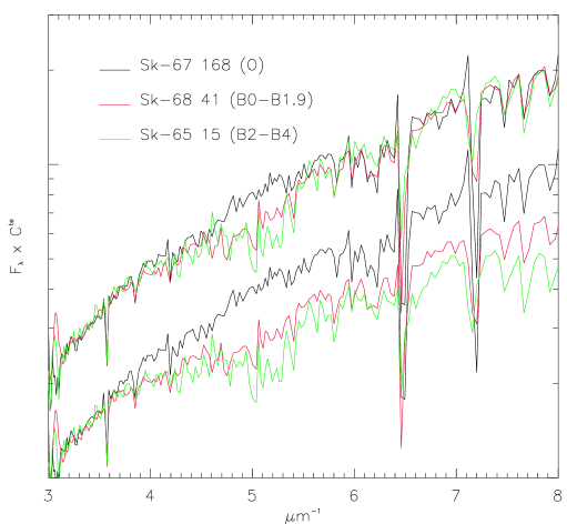
Figure 3: Bottom spectra are IUE spectra of Sk-67 168 (O type, black line), Sk-68 41 (B0-B1.9, red line), Sk-65 15 (B2-B4, green line), scaled to the same arbitrary value in the near-UV. Top, spectra of Sk-68 41 and of Sk-65 15 have been multiplied respectively by $e^{0.08/\lambda}$ and by $e^{0.14/\lambda}$, to match the slope of the spectrum of Sk-67 168. Y-logarithmic axis.

5 Stars with no $2200\,\rm\AA$ bump, and $B-V>0$

A few LMC/SMC stars have a positive $B-V$ (which for these O-B stars is proof of a non negligible reddening) and, contrary to common Galactic stars with similar reddening, have no $2200\,\rm\AA$ bump. These are AzV398 O), AzV18 and AzV214 (B0-B1.9), in the SMC; Sk-69 228, Sk-69 256, and Sk-70 116 (B2-B4), in the LMC (Figure 4). $E(B-V)$ ranges from 0.2 to 0.4 mag., significantly larger than for the slightly reddenned stars of Sect. 4.

Normalisation of the UV spectra of the stars (Figure 5) by the low reddened ones of Sect. 4, of same type, gives in the near-UV an exponential of $1/\lambda$ (the exponent $\Delta_{uv}$ is written on each plot).

For three of the stars (Sk-69 256, AzV214, AzV18) this exponential can be prolonged to the far-UV. The increase of reddening from Sk-69 256 to AzV18 is clearly observed through the progressive change of slope from one reduced spectrum to the other (Figure 5). There is excellent agreement between $\Delta_{uv}$ and $\Delta_{vis}$: the extinction law in these directions is linear from the visible to the far-UV, and, as in Sect. 4, Galactic and Magellanic extinctions along these lines of sight can not be distinguished.

For AzV398, Sk-69 228 and Sk-70 116, $\Delta_{vis}$ is still a good indicator of the difference of near-UV slope with stars of lesser reddening, but in the far-UV the SEDs ratios are in excess compared to the visible slopes. The exact wavelength from which the curves depart from linearity is not clear (especially for Sk-70 116) owing to the overlap between the bump and the AL/Fe absorption regions.

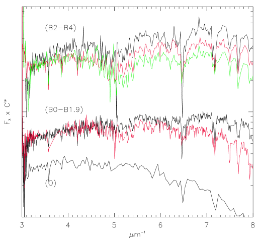
Figure 4: UV spectra of reddened stars, with $B-V>0$ and no $2200\,\rm\AA$ bump (Sect. 5). AzV398 is the only O star. B0-B1.9 stars are AzV18 (in red) and AzV214 (in black). B2-B4 are Sk-69 256 (black line), Sk-69 228 (red line), Sk-70 116 (green line). Y-logarithmic axis.

Figure 5: Reduced spectra for the stars of Figure 4, Y-logarithmic axis. The straight line on each plot, with slope $\Delta_{uv}$, prolongs the visible extinction. The y-axis spans a factor of 10 for all but AzV398 plots, a factor of 15 for AzV398’s.

6 Reddened stars with a $2200\,\rm\AA$ bump

Reddened stars with a $2200\,\rm\AA$ bump are all but one (AzV398) in the LMC. They will be distinguished according to their spectral type and to the size of the bump (weak or large).

6.1 Weak bumps

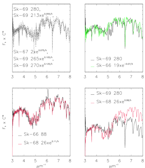
Figure 6: Stars with a weak bump (Sect. 6.1). Y-logarithmic axis.

Among the twelve stars with a weak bump (quoted by a ’W’, last column in Tables 1 and 2), nine [Sk-68 155 (O), Sk-66 19, Sk-68 129, Sk-68 140 (B0-B1.9), Sk-69 213, Sk-69 280, Sk-67 2, Sk-69 265, Sk-69 270 (B2-B4)] have UV spectra which differ exactly by a change of slope (an exponential of $1/\lambda$, Figure 6, top plots). The correspondence between the change of slope in the visible and in the UV between the stars (last column of Table 4) is excellent for all stars but Sk-66 19. Along all these directions (except Sk-66 19) reduced spectra will differ by an exponential of $1/\lambda$, and the extinction laws by a linear term, over all the visible-UV wavelength range.

The UV spectra of Sk-66 19 and of Sk-69 280 superimpose perfectly with a slight change of slope (right top plot of Figure 6). A break of this change of slope between the visible and the near-UV can not be excluded although it would represent an exception among the stars considered so far. On the other hand, a slightly larger error than expected in Sk-66 19’s photometry, or the possibility that $B-V$ does not properly represent its slope would explain the discrepancy. A comparison of the visible SEDs of the stars would best fix this problem.

B2-B4 stars Sk-66 88, Sk-68 26, AzV456, lie apart. Their visible/UV spectra differ one from another by a change of slope, which is equal (within the error-margins) in the visible and in the UV (Table 4). Their UV spectra do not match the preceding ones, whichever correction of the slope is applied: if, for instance, the UV spectrum of Sk-66 88, corrected for the difference of slope given by the visible photometry, is compared to the spectrum of Sk-68 129 (Figure 6, bottom right plot), large differences appear in the far-UV part of the spectra (the bump may also be smaller for Sk-66 88 than it is for Sk-68 129). The implication, already apparent in Sect. 5, is that visible extinction alone does not suffice to fix the extinction in the UV. One additional parameter, at least, is necessary. However linear extinction laws still play a role in these directions of higher extinction since the visible-UV spectra of many of them deduce one from the other by an exponential of $1/\lambda$.

Table 4: Stars with a weak bump ($0.15<B-V<0.4$)

star type $$\Delta_{vis}^{(1)}$$

Sk-68 155 O -0.06 -0.05 -0.01

Sk-66 19 B0-B1.9 0.06 -0.07 0.13

Sk-68 129 B0-B1.9 -0.12 -0.15 -0.03

Sk-68 140 B0-B1.9 0.00 0.06 -0.06

Sk-69 280 B2-B4 0 0 0

Sk-69 213 B2-B4 0.02 0.05 -0.03

Sk-67 2 B2-B4 0.02 0.07 -0.05

Sk-69 265 B2-B4 0.06 0.10 -0.04

Sk-69 270 B2-B4 0.10 0.12 -0.02

Sk-68 26 B2-B4 0 0 0

Sk-66 88 B2-B4 0.14 0.11 0.04

AzV 456 B0-B1.9 -0.06 -0.07 -0.01

• Twice the difference of B-V between the star and the star chosen as reference (the star with $\Delta_{vis}=\Delta_{uv}=0$).

• Difference of UV slopes between the star and the reference one.

6.2 Large bumps

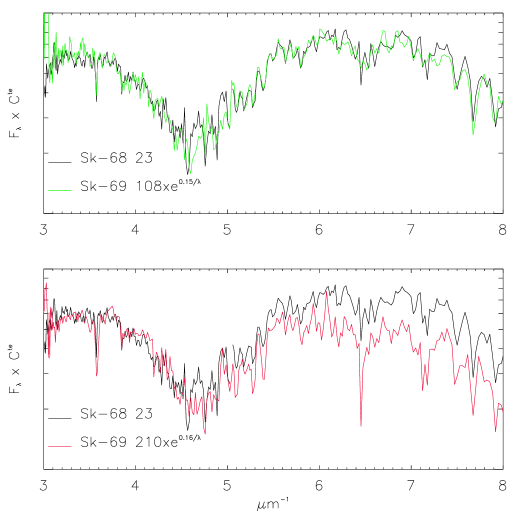
Figure 7: Stars with a large bump (Sect. 6.2). Y-logarithmic axis.

Most pronounced bumps are observed in the spectra of B2-B4 stars with relatively high reddenings ($E(B-V)\sim 0.5$) Sk-68 23, Sk-69 108, and Sk-69 210.

Sk-69 108 and Sk-68 23 have a slightly larger bump than Sk-69 210. Their UV spectra differ by an exponential $e^{0.15/\lambda}$, the exponent being close to the change of visible slope $\Delta_{vis}\sim 0.10$ (Figure 7, top).

The bottom plot of Figure 7 proves that the UV spectra of Sk-68 23 and Sk-69 210 superimpose well in the near-UV, after the slope of the latter has been corrected for the difference of visible reddening, but the spectra do not match in the far-UV. There is no straightforward relationship between the variation of the extinction curve in the visible and in the UV between the directions of Sk-69 210 on the one hand, and Sk-68 23 and Sk-69 108 on the other.

7 Fit of LMC/SMC extinction curves

7.1 The CCM parametrization

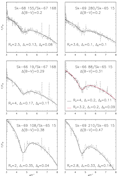
Figure 8: Fit (Eq. 7) of the reduced spectra of a representative set of Magellanic stars with a bump (Sect. 7.2). Y-logarithmic axis.

Figures 1 and 2 in CCM demonstrate that the different parts of Galactic extinction curves vary simultaneously, in a systematic way, depending on $E(B-V)$ and one additional parameter only: at all wavelengths and for all directions, there is a linear relationship between $A_{\lambda}/E(B-V)$ and $R_{V}^{-1}=A_{V}/E(B-V)$. Since $E(B-V)$ can be simplified between these two expressions, the CCM finding means that $A_{\lambda}$ is not determined by $E(B-V)$ alone, but is a linear combination of $E(B-V)$ and $A_{V}$. In other words, the exact shape of the extinction curve of an average Galactic star is fixed by the visible reddening, and the knowledge of one point (here ($\lambda_{V},A_{V}$)) in the $(1/\lambda,\,A_{\lambda})$ plane. The mathematical transcription of the CCM finding is that there are two functions $a(x)$ and $b(x)$ which satisfy

$$\frac{A_{\lambda}}{A_{V}} = a(x)+b(x)R_{V}^{-1}$$

(eq. 1 in CCM, $x=1/\lambda$) or

$$A_{\lambda} = a(x)A_{V}+b(x)E(B-V)$$ (5)

$$= E(B-V)(a(x)R_{V}+b(x))$$

In the UV $a(x)$ and $b(x)$ are given by eqs. 4a and 4b in CCM

$$a(x) = 1,752-0.316-\frac{0.104}{(x-4.67)^{2}+0.341}+F_{a}(x)$$

$$b(x) = -3.090+1.825x+\frac{1.206}{(x-4.62)^{2}+0.263}+F_{b}(x)$$

with

$$F_{a}(x) = -0.0447(x-5.9)^{2}-0.009779(x-5.9)^{3}$$

$$(8\geq x\geq 5.9)$$

$$F_{b}(x) = 0.2130(x-5.9)^{2}+0.1207(x-5.9)^{3}$$

$$(8\geq x\geq 5.9)$$

$$F_{a}(x) = F_{b}(x)=0$$

$$(x<5.9)$$

Eq. 5 is equivalent to

$$\frac{F_{\star}}{F_{0}} = Ce^{-0.92E(B-V)(b+aR_{V})}$$ (6)

$$= Ce^{-0.92E(B-V)b(x)}e^{-0.92E(B-V)R_{V}a(x)}$$

($F_{\star}$ and $F_{0}$ are the reddened and the reference stars spectra, $C$ a constant).

Two remarks should be made. One is that in practice, taking the $a(x)$ and $b(x)$ functions given in CCM (and reproduced above), the information on the $2200\,\rm\AA$ bump feature is nearly all contained in the first exponential of Eq. 6, which fixes the size of the bump, and an average slope for the extinction curve. Therefore, in the CCM framework, the bump depends mainly on $E(B-V)$ (almost not on $R_{V}$), an hypothesis only partially confirmed by observation (Savage, 1975). The second exponential, thus the value of $R_{V}$, allows some variation of the UV curve’s slope around the mean slope.

The second point that we must draw attention to is that linear extinction laws in the UV, as they were encountered in previous sections, are not accounted for by the CCM fit: it would require the exponent involving $b(x)$ to be null (no bump), and thus: $E(B-V)=0$. Therefore most of SMC extinction curves, and Galactic sight-lines of very low column densities (Zagury, 2001) will not be fitted by the CCM relationship.

7.2 Fit of extinction curves

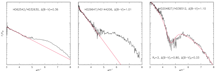
Figure 9: Reduced spectra of Milky Way stars which do not follow the CCM relationship (Valencic et al., 2004) (Sect. 7.3). The straight line on the two first plots is the UV prolongation of the visible extinction. HD204827 is fitted by Equation 7. Y-logarithmic axis.

Gordon et al. (2003) finds that four directions only, out of the forty one of the sample, Sk-69 280, Sk-66 19 (weak bump, Sect. 6.1), Sk-68 23, Sk-69 108 (large bump, Sect. 6.2) follow a CCM relationship (with respective $R_{V}$ of 3.12, 3.44, 3.55, 3.15). It follows from Sect. 6 that all stars with a bump whose spectra differ from these four ones by a change of slope only (an exponential of $1/\lambda$ over all the visible wavelength range) will have their reduced spectrum fitted by the product of a CCM fit (Eq. 6) and an exponential of $1/\lambda$: the extinction law in these directions (that is all directions with a bump except these of Sk-68 26, Sk-66 88, AzV456, Sk-69 210 and maybe Sk-66 19) is the sum of a CCM and a linear extinction laws. For these directions, it is possible to find $\Delta_{1}$ and $\Delta_{2}$ for which

$$\frac{F_{\star}}{F_{0}} = Ce^{-0.92\Delta_{1}(b+aR_{V})}e^{-2\Delta_{2}/\lambda}$$ (7)

$$= Ce^{-0.92\Delta_{1}b(x)}e^{-0.92\Delta_{1}R_{V}a(x)}e^{-2\Delta_{2}/\lambda},$$

with $\Delta_{1}+\Delta_{2}\sim\Delta(B-V)$.

From Figure 8 it will be concluded that this fit also applies to Sk-66 19, Sk-68 26 (thus also to Sk-66 88, AzV456, Sect. 6.1) and to Sk-69 210. Since it holds for directions with a linear extinction, it finally applies to all forty one stars of the sample, with the exception of Sk-69 228, Sk-70 116, and AzV398 which do not exhibit the bump feature and do not have a linear extinction.

$\Delta_{1}$ in Eq. 7 is unambiguously fixed by the strength of the $2200\,\rm\AA$ bump, $\Delta_{2}$ by the difference between $\Delta(B-V)$ and $\Delta_{1}$. $R_{V}$ then adjusts the UV slope of the fit, as in the CCM framework (Sect. 7.1).

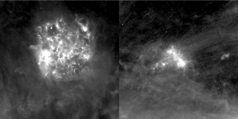
Figure 10: IRAS $100\,\rm\mu m$ images (gnomonic J2000 coordinates, 1 pix=90", each field is $12.5^{\circ}\times 12.5^{\circ}$ wide) of the LMC (left) and the SMC (right) (from Sky-View). The field, larger than the extent of the galaxies, includes the Galactic cirrus on each line of sight. Cutoffs are 1.5 MJy/sr and 100 MJy/sr for the LMC, 0.5 and 30 MJy/sr for the SMC. Logarithmic scale.

The expression of a normalized extinction curve can easily be retrieved from Eq. 7:

$$\frac{A_{\lambda}}{E(B-V)} = \frac{\Delta_{1}}{E(B-V)}(a(x)R_{V}+b(x))$$ (8)

$$+\,0.53(1-\frac{\Delta_{1}}{E(B-V)})x,$$

$\Delta_{1}$ being unequivocally determined by the size of the $2200\,\rm\AA$ bump.

7.3 Remarks on Eqs. 7 and 8

Eq. 7 (or 8) separates, along each sight-line, a CCM component from a linear component. As in CCM, the bump size is associated with a value ($\Delta_{1}$) of the reddening although, in this new formulation, it may be only part of $E(B-V)$. The remaining part ($\Delta_{2}=E(B-V)-\Delta_{1}$) of $E(B-V)$ follows a linear extinction law. The correspondence between $E(B-V)$ and bump size, implicit in CCM, is thus a boarder case ($\Delta_{1}\rightarrow E(B-V)$, $\Delta_{2}\rightarrow 0)$, rather than the generality.

Firstly, this allows one to account for linear extinction curves. Secondly, it allows a fit of most Galactic and Magellanic extinction curves by a single, common mathematical expression. For a given bump size the number of free parameters of a normalized extinction curve remains unchanged (= 1).

There is, for this fit as well as for CCM’s, a large uncertainty on the value of $R_{V}$ due to the uncertainty on $\Delta(B-V)$: middle right plot of Figure 8 gives two acceptable and nearly undistinguishable fits of the UV spectrum of Sk-66 88 which differ by $\Delta(B-V)=0.02$ while the values found for $R_{V}$ vary from 3.2 to 4; any small uncertainty on $\Delta(B-V)$ leads to a large variation of $R_{V}$. The sensitivity of the $R_{V}$ parameter to the reference star is also indicated by a comparison of the values given in Gordon et al. (2003) to the ones found here: for Sk-66 19, for instance, with Sk-66 169 as comparison, Gordon et al. (2003) finds $R_{V}=3.44\pm 0.21$ while the present decomposition, with Sk-67 168 as reference, gives $R_{V}\sim 4$. Noteworthy, Bouchet et al. (1985) finds, from a multi-wavelength analysis, $R_{V}=2.7\pm 0.2$ in the SMC.

Eq. 7 can be used to re-examine particular Galactic extinction curves. Only four directions out of the 417 studied by Valencic et al. (2004) do not follow a CCM relationship. The reduced spectra of three [HD62542 ($E(B-V)=0.38$), HD204827 ($E(B-V)=0.80$), HD29647 ($E(B-V)=0.91$] of these directions (the fourth, HD210121, is not considered here because its spectral type and $B-V$ color are poorly known) are plotted on Figure 9. HD204827 has a bump and is well fitted using Eq. 7 with $R_{V}\sim 3$. The two other directions, HD62542 and HD29647, have no or little bump, and their near-UV reduced spectra prolong the visible extinction law, the far-UV part being in excess. As Sk-69 228, Sk-70 116, AzV398 they can not be fitted by Eq. 7.

8 On the separation of Galactic and Magellanic extinctions

Sects. 4, 5, and 7.2 demonstrate that it is not possible to separate analytically Galactic and Magellanic extinctions. An attempt to bypass this difficulty is made in Misselt et al. (1999): reddened stars in the LMC are associated to reference stars with a similar Galactic reddening, estimated from the Ostreicher et al. (1995) $10^{\prime}$ resolution Galactic map. According to this paper the resulting extinction curves isolate the Magellanic extinction.

Both the LMC and the SMC are observed behind Galactic cirrus. The highlighted infrared (filamentary) structures (see Figure 10, retrieved from Sky-View at http://skys.gsfc.nasa.gov) observed in the direction of the Clouds belong to the Galaxy: they reproduce the structure of all Galactic cirrus observed by IRAS; there is continuity between the filaments in and outside the Magellanic Clouds (Figure 11); and it would be remarkable that such structures, which would represent enormous masses of gas at the distance of the Magellanic Clouds, can mimic so well Galactic cirrus (unless one supposes self-similarity of cirrus up to very large scales). The large infrared surface brightness at their position results from the strong infrared gradients due to dust surrounding the Magellanic giant stars, over-which is superimposed the much lower Galactic HLC emission.

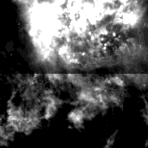
Figure 11: Bottom two thirds of LMC image (Figure 10), with different cutoffs (3 and 10 MJy/sr for the lowest part, 3 and 30 MJy/sr for the upper one). There is continuity of the infrared structures in and out of the LMC.

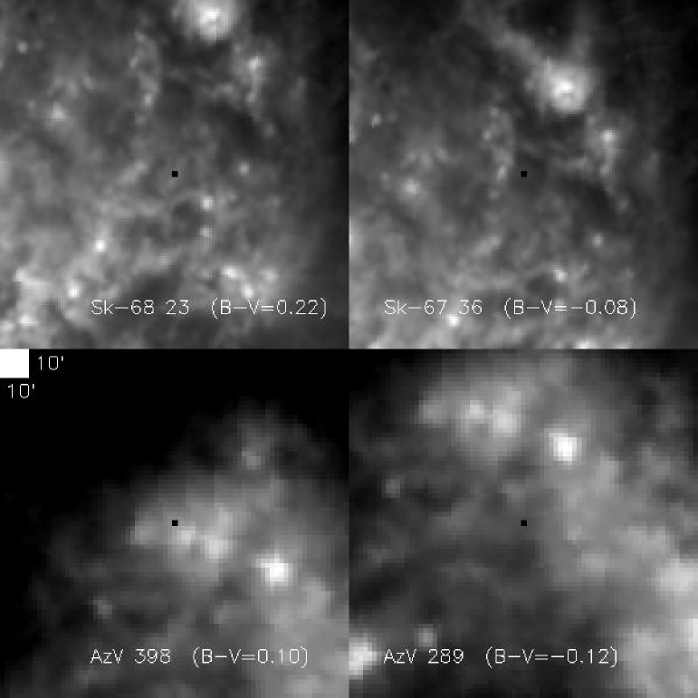
Figure 12: Four times magnified IRAS $100\,\rm\mu m$ images (from Sky-View) centered on reddened Sk-68 23 (top left) and AzV 398 (bottom left), and their comparison stars in Gordon et al. (2003), Sk-67 36 (top right) and AzV 289 (bottom right). Each image is $1.87^{\circ}\times 1.87^{\circ}$ wide, cutoffs are identical for reddened and comparison star images. The beam of Ostreicher et al. (1995) extinction map is given by the bright square top left of the left bottom image.

It will be deduced that the Galactic extinction map in these directions is structured down to very small scales: at least the one arcminute probed by IRAS images, and most probably to sub-arcseconds as it can be observed on visible images of Galactic cirrus (Zagury et al., 1999). The relative positions of the Magellanic stars and of Galactic structures on IRAS maps can serve as an indicator of the different amounts of Galactic dust along the stars’ directions. Figure 12 compares the $100\,\rm\mu m$ emission around reddened Sk-68 23 (top left) and AzV 398 (bottom left), and the comparison stars adopted in Gordon et al. (2003), respectively Sk-67 36 (top right) and AzV 289 (bottom right). In both cases the reddened stars are situated behind local enhancements of Galactic interstellar matter, while the comparison stars are seen through ’holes’ (presumably) of much lower column densities. The $10^{\prime}$ resolution (see Figure 12) of the Ostreicher et al. (1995) Galactic extinction map in the direction of the LMC lacks the precision needed to resolve the structure of Galactic cirrus on the line of sight, and is therefore of no help in separating Galactic and LMC extinctions.

The relationship between Galactic cirrus and Magellanic sight-lines can be investigated at an even smaller scale with the Palomar visible plates (DSS2 blue plates, available at Sky-View). The plates show, in and around the Magellanic Clouds, nebulosities which ’zoom’ into the infrared filaments and reveal the Galactic structures at a $\sim 1^{\prime\prime}$ scale. The source of illumination of these nebulosities could be the Magellanic Clouds themselves (Zagury, 2000b), which are the strongest source of visible light in the region. Most of the Magellanic stars with a bump are observed behind such nebulosities (see for instance the LMC DSS2 blue images around Sk-68 155, Sk-68 140, Sk-69 213, Sk-69 270, Sk-69 206).

The separation between Galactic and Magellanic extinctions seems to be out of reach from up to date observations. It can not be excluded for example that the $2200\,\rm\AA$ bump observed in some Magellanic directions is due to Galactic cirrus on the lines of sight, while Magellanic extinction laws are always linear. This would explain why the bump is more frequently observed towards the LMC than towards the SMC, since the cirrus in front of the LMC has an average column density ($E(B-V)\sim 0.075$, $A_{V}\sim 0.25$, Schlegel et al. (1998)) about twice that of the cirrus in front of the SMC ($E(B-V)\sim 0.037$, $A_{V}\sim 0.12$). In this case Magellanic extinction laws would resumed to the linear part of the extinction curves.

9 Conclusion

Previous works on Magellanic extinction based on UV extinction curves all find major differences between the characteristics of extinction in the SMC, the LMC, and the Milky Way. In contrast, the present analysis shows that there is no proof, up to date, of a different nature of the extinction in the Magellanic Clouds and in the Galaxy, and therefore that there is no reason, from the sole study of extinction curves, to suppose a variation of grain composition between these galaxies. This analysis also highlights the important role linear extinction laws play, even in high column density directions. A generalization of the CCM fit, which still depends upon a single parameter for a given size of the $2200\,\rm\AA$ bump, was found and applies, in all three galaxies, to all directions except the ’transition’ ones where the linear visible reddening law breaks in the far-UV only, and where no $2200\,\rm\AA$ bump is found.

This study first proved (Sects. 4 and 5) that, in SMC/LMC low column density directions, Magellanic and Galactic extinction laws are linear and can not be distinguished. Combined with the Zagury (2001) finding of linear extinction laws in Galactic slightly reddened directions, it implies that linearity over all the visible/UV wavelength range in low column density directions characterizes interstellar extinction in all three galaxies. As column density increases, linearity breaks first in the far-UV, as an excess of light appears in some sight-lines. For the highest column densities, extinction is less than expected by the prolongation of the linear visible rise in the UV, and the traditional UV extinction features progressively appear. There are no fixed thresholds between these transitions in the shape of the extinction curve. For example, linearity seems to hold at larger $E(B-V)$ in the SMC than in the Milky Way.

These ostensibly unpredictable behaviors are described by relationships which, surprisingly, involve a very small number of parameters. In 1989 the CCM article first proved that a large set of normalized extinction curves is accounted for by a single parameter law. This law however is not followed by all extinction curves: linear extinction curves in particular, which characterize the SMC but are also present in the Milky Way, can not be fitted using the CCM law (Sect. 7.1). To embrace an even larger set of extinction curves it is necessary to give up the correspondence, implicit in CCM, between E(B-V) and bump size. The reddening in any one direction can then be separated into two parts, one following the CCM extinction law, the other a linear one. This generalization of the CCM fit is given by Eq. 7 (Eq. 8 for normalized extinction curves). It applies to all Galactic and Magellanic directions except those which have no $2200\,\rm\AA$ bump and depart from linearity in the far-UV.

That some directions do not follow the generalized CCM relationship of Sect. 7.2 should simply be attributed to its lack of physical foundations. The large uncertainties on the parameter $R_{V}$ derived from this fit, its role in Eq. 7 (it affects only the UV part of the fits) question, in my opinion, the physical meaning of $R_{V}$ derived from either the CCM fit or from Eqs. 7 and 8.

It is therefore not possible from the data in hand to infer differences between Magellanic and Galactic dusts. It is also not possible for directions with a linear extinction law to get any precise information on the chemical composition of the dust: even atmospheric aerosols lead to such laws. Linear extinction is an ubiquitous phenomenon in Nature which provides information on the grain size distribution, but not on the grains’ composition.

This study highlights a general coexistence of linear and non-linear components in interstellar extinction laws, which, along with the passage from linearity to CCM extinction curves remain to be understood. It could be that both types of extinction coexist along some sight-lines, and one could imagine that in the direction of the Magellanic Clouds, the Magellanic extinction law is linear (as it was suggested for the SMC by Prévot et al. (1984)) while the Galactic law is CCM-like. This can not be a complete and satisfactory answer however since it does not help our understanding of the intermediate stage of extinction, where linearity extends in the near-UV only, nor does it explain the role of linear extinction laws in the Galaxy. The solution should come from a better understanding of these transition directions and will probably imply a re-consideration of the nature of interstellar extinction, in particular the advent of a fit based on a physical understanding of the phenomena at work.

References

- Ardeberg et al. (1972) Ardeberg, A., Brunet, J.P., Maurice, E., Prévot, L. 1972, A&AS, 6, 249
- Ardeberg & Maurice (1977) Ardeberg, A., Maurice, E. 1977, A&AS, 30, 261
- Azzopardi et al. (1975) Azzopardi, M., Vigneau, J., Macquet, M. 1975, A&AS, 22, 285
- Azzopardi & Vigneau (1982) Azzopardi, M., Vigneau J. 1982, A&AS, 50, 291
- Bouchet et al. (1985) Bouchet, P., Lequeux, J., Maurice, E., Prévot, L., Prévot-Burnichon, M.L. 1985, A&A, 149, 330
- Cardelli et al. (1989) Cardelli, J.A., Clayton, G.C., Mathis, J.S. 1989, ApJ, 345, 245
- Cartledge et al. (2005) Cartledge, S.I.B., et al. 2005, ApJ, 630, 355
- Clayton et al. (2000) Clayton, G.C., Gordon, K.D., Wolff, M.J. 2000 ApJSS, 129, 147
- Desert et al. (1990) Desert, F.-X., Boulanger, F., Puget, J.L. 1990, A&A, 237, 215
- Divan (1954) Divan, L. 1954, AnAp, 17, 456
- Fitzgerald (1970) FitzGerald, M. P. 1970, A&A, 4, 234
- Fitzpatrick (1988) Fitzpatrick, E.L. 1988, ApJ, 335, 703
- Gordon et al. (2003) Gordon, K.D., Clayton, G.C., Misselt, K.A., Landolt, A.U., Wolff, M.J. 2003, ApJ, 594, 279
- Hall (1937) Hall, J.S. 1937, ApJ, 85, 145
- Henyey & Greenstein (1941) Henyey, L.C., Greenstein, J.L. 1941, ApJ, 93, 70
- Isserstedt (1975) Isserstedt, J. 1975, A&AS, 19, 259
- Isserstedt (1979) Isserstedt, J. 1979, A&AS, 38, 239
- Isserstedt (1982) Isserstedt, J. 1982, A&AS, 50, 7
- Garmany et al. (1995) Garmany, C. D., Conti, P., Massey, P. 1987, AJ, 93, 5
- Misselt et al. (1999) Misselt, K.A., Clayton, G.C., Gordon, K. D. 1999, ApJ, 515, 128
- Nicolet (1978) Nicolet, B. 1978, A&AS, 34, 1
- Ostreicher et al. (1995) Osteicher, M. O., Gochermann, J., Schmidt-Kaler, T. 1995, A&ASS, 112, 495
- Prévot et al. (1984) Prévot, M. L., Lequeux, J., Maurice, E., Prévot, L., Rocca-Volmerange, B. 1984, A&A, 132, 389
- Rousseau et al. (1978) Rousseau, J., Martin, N., Prévot, L., Rebeirot, E., Robin, A., Brunet, J. P. 1978, A&AS, 31, 243
- Savage (1975) Savage, B. D. 1975, ApJ, 199, 92
- Schlegel et al. (1998) Schlegel, D., Finkbeiner, D. P., Davis, M. 1998, ApJ, 500, 525
- Smith Neubig & Bruhweiler (1997) Smith Neubig, M. M., Bruhweiler, F. C. 1997, AJ, 114, 1951
- Smith Neubig & Bruhweiler (1999) Smith Neubig, M. M., Bruhweiler, F. C. 1999, AJ, 117, 2856
- Stebbins et al. (1939) Stebbins, J., Huffer, C .M., Whitford, A. E. 1939, ApJ, 90, 209
- Valencic et al. (2004) Valencic, L. A. , Clayton, G. C., Gordon, K. D. 2003, ApJ, 594, 279
- Zagury et al. (1999) Zagury, F., Boulanger, F., Banchet, V. 1999, A&A, 352, 645
- Zagury (2000a) Zagury, F. 2000, NewA, 5, 211
- Zagury (2000b) Zagury, F. 2000, NewA, 5, 367
- Zagury (2001) Zagury, F. 2001, NewA, 6, 471