Geometric Complexity Theory: Introduction

Foreword

These are lectures notes for the introductory graduate courses on geometric complexity theory (GCT) in the computer science department, the university of Chicago. Part I consists of the lecture notes for the course given by the first author in the spring quarter, 2007. It gives introduction to the basic structure of GCT. Part II consists of the lecture notes for the course given by the second author in the spring quarter, 2003. It gives introduction to invariant theory with a view towards GCT. No background in algebraic geometry or representation theory is assumed. These lecture notes in conjunction with the article [GCTflip1], which describes in detail the basic plan of GCT based on the principle called the flip, should provide a high level picture of GCT assuming familiarity with only basic notions of algebra, such as groups, rings, fields etc. Many of the theorems in these lecture notes are stated without proofs, but after giving enough motivation so that they can be taken on faith. For the readers interested in further study, Figure 1 shows logical dependence among the various papers of GCT and a suggested reading sequence.

The first author is grateful to Paolo Codenotti, Joshua Grochow, Sourav Chakraborty and Hari Narayanan for taking notes for his lectures.

$$\begin{array}[]{ccc}\framebox{\parbox{54.2025pt}{GCTabs}}\\ |\\ \downarrow\\ \framebox{GCTflip1}\\ |\\ \downarrow\\ \framebox{These lecture notes}&--\rightarrow&\framebox{GCT3}\\ |&&|\\ \downarrow&&|\\ \framebox{GCT1}&&|\\ |&&|\\ \downarrow&&|\\ \framebox{GCT2}&&|\\ |&&|\\ \downarrow&&\downarrow\\ \framebox{GCT6}&\leftarrow--&\framebox{GCT5}\\ |\\ \downarrow\\ \framebox{GCT4}&--\rightarrow&\framebox{GCT9}\\ |\\ \downarrow\\ \framebox{GCT7}\\ |\\ \downarrow\\ \framebox{GCT8}\\ |\\ \downarrow\\ \framebox{GCT10}\\ |\\ \downarrow\\ \framebox{GCT11}\\ |\\ \downarrow\\ \framebox{GCTflip2}\\ \end{array}$$

Figure 1: Logical dependence among the GCT papers

Part I The basic structure of GCT
By Ketan D. Mulmuley

Chapter 1 Overview

Scribe: Joshua A. Grochow

Goal: An overview of GCT.

The purpose of this course is to give an introduction to Geometric Complexity Theory (GCT), which is an approach to proving $\mbox{{P}}\neq\mbox{{NP}}$ via algebraic geometry and representation theory. A basic plan of this approach is described in [GCTflip1, GCTflip2]. It is partially implemented in a series of articles [GCT1]-[GCT11]. The paper [GCTconf] is a conference announcement of GCT. The paper [Ml] gives an unconditional lower bound in a PRAM model without bit operations based on elementary algebraic geometry, and was a starting point for the GCT investigation via algebraic geometry.

The only mathematical prerequisites for this course are a basic knowledge of abstract algebra (groups, ring, fields, etc.) and a knowledge of computational complexity. In the first month we plan to cover the representation theory of finite groups, the symmetric group $S_{n}$, and $GL_{n}(\mathbb{C})$, and enough algebraic geometry so that in the remaining lectures we can cover basic GCT. Most of the background results will only be sketched or omitted.

This lecture uses slightly more algebraic geometry and representation theory than the reader is assumed to know in order to give a more complete picture of GCT. As the course continues, we will cover this material.

1.1 Outline

Here is an outline of the GCT approach. Consider the P vs. NP question in characteristic 0; i.e., over integers. So bit operations are not allowed, and basic operations on integers are considered to take constant time. For a similar approach in nonzero characteristic (characteristic 2 being the classical case from a computational complexity point of view), see GCT 11.

The basic principle of GCT is the called the flip [GCTflip1]. It “reduces” (in essence, not formally) the lower bound problems such as P vs. NP in characteristic 0 to upper bound problems: showing that certain decision problems in algebraic geometry and representation theory belong to $P$. Each of these decision problems is of the form: is a given (nonnegative) structural constant associated to some algebro-geometric or representation theoretic object nonzero? This is akin to the decision problem: given a matrix, is its permanent nonzero? (We know how to solve this particular problem in polynomial time via reduction to the perfect matching problem.)

Next, the preceding upper bound problems are reduced to purely mathematical positivity hypotheses [GCT6]. The goal is to show that these and other auxilliary structural constants have positive formulae. By a positive formula we mean a formula that does not involve any alternating signs like the usual positive formula for the permanent; in contrast the usual formula for the determinant involves alternating signs.

Finally, these positivity hypotheses are “reduced” to conjectures in the theory of quantum groups [GCT6, GCT7, GCT8, GCT10] intimately related to the Riemann hypothesis over finite fields proved in [Dl2], and the related works [BBD, KL2, Lu2]. A pictorial summary of the GCT approach is shown in Figure 1.1, where the arrows represent reductions, rather than implications.

$$\begin{array}[]{ccccc}\begin{array}[]{|c|}\hline\cr\\ \mbox{P vs. NP}\\ \mbox{char. 0}\\ \\ \hline\cr\end{array}&\begin{array}[]{c}\mbox{{\Large Flip}}\\ \Longrightarrow\end{array}&\begin{array}[]{|c|}\hline\cr\\ \mbox{Decision problems}\\ \mbox{in alg. geom.}\\ \mbox{\& rep. thy.}\\ \\ \hline\cr\end{array}&\Longrightarrow&\begin{array}[]{|c|}\hline\cr\\ \mbox{Show certain}\\ \mbox{constants in alg.}\\ \mbox{geom. and repr.}\\ \mbox{theory have}\\ \mbox{positive formulae}\\ \\ \hline\cr\end{array}\\ \begin{array}[]{c}\mbox{Lower bounds}\\ \mbox{(Neg. hypothesis}\\ \mbox{in complexity thy.)}\end{array}&&\begin{array}[]{c}\mbox{Upper bounds}\\ \mbox{(Pos. hypotheses}\\ \mbox{in complexity thy.)}\end{array}&&\begin{array}[]{c}\mbox{Pos. hypotheses}\\ \mbox{in mathematics}\end{array}\\ \\ &\Longrightarrow&\begin{array}[]{|c|}\hline\cr\\ \mbox{Conjectures on }\\ \mbox{quantum groups}\\ \mbox{related to RH over}\\ \mbox{finite fields}\\ \\ \hline\cr\end{array}\end{array}$$

Figure 1.1: The basic approach of GCT

To recap: we move from a negative hypothesis in complexity theory (that there does not exist a polynomial time algorithm for an NP-complete problem) to a positive hypotheses in complexity theory (that there exist polynomial-time algorithms for certain decision problems) to positive hypotheses in mathematics (that certain structural constants have positive formulae) to conjectures on quantum groups related to the Riemann hypothesis over finite fields, the related works and their possible extensions. The first reduction here is the flip: we reduce a question about lower bounds, which are notoriously difficult, to the one about upper bounds, which we have a much better handle on. This flip from negative to positive is already present in Gödel’s work: to show something is impossible it suffices to show that something else is possible. This was one of the motivations for the GCT approach. The Gödelian flip would not work for the P vs. NP problem because it relativizes. We can think of GCT as a form of nonrelativizable (and non-naturalizable, if reader knows what that means) diagonalization.

In summary, this approach very roughly “reduces” the lower bound problems such as P vs. NP in characteristic zero to as-yet-unproved quantum-group-conjectures related to the Riemann Hypothesis over finite fields. As with the classical RH, there is experimental evidence to suggest these conjectures hold – which indirectly suggests that certain generalizations of the Riemann hypothesis over finite fields also hold – and there are hints on how the problem might be attacked. See [GCTflip1, GCT6, GCT7, GCT8] for a more detailed exposition.

1.2 The Gödelian Flip

We now re-visit Gödel’s original flip in modern language to get the flavor of the GCT flip.

Gödel set out to answer the question:

Q: Is truth provable?

But what “truth” and “provable” means here is not so obvious a priori. We start by setting the stage: in any mathematical theory, we have the syntax (i.e. the language used) and the semantics (the domain of discussion). In this case, we have:

Syntax (language)	Semantics (domain)
First order logic
($\forall,\exists,\neg,\vee,\wedge,\dots$)
Constants	0,1
Variables	$x,y,z,\dots$
Basic Predicates	$>$, $<$, $=$
Functions	$+$,$-$,$\times$,exponentiation
Axioms	Axioms of the natural numbers $\mathbb{N}$
	Universe: $\mathbb{N}$

A sentence is a valid formula with all variables quantified, and by a truth we mean a sentence that is true in the domain. By a proof we mean a valid deduction based on standard rules of inference and the axioms of the domain, whose final result is the desired statement.

Hilbert’s program asked for an algorithm that, given a sentence in number theory, decides whether it is true or false. A special case of this is Hilbert’s 10th problem, which asked for an algorithm to decide whether a Diophantine equation (equation with only integer coefficients) has a nonzero integer solution. Gödel showed that Hilbert’s general program was not achievable. The tenth problem remained unresolved until 1970, at which point Matiyasevich showed its impossibility as well.

Here is the main idea of Gödel’s proof, re-cast in modern language. For a Turing Machine $M$, whether the empty string $\varepsilon$ is in the language $L(M)$ recognized by $M$ is undecidable. The idea is to reduce a question of the form $\varepsilon\in L(M)$ to a question in number theory. If there were an algorithm for deciding the truth of number-theoretic statements, it would give an algorithm for the above Turing machine problem, which we know does not exist.

The basic idea of the reduction is similar to the one in Cook’s proof that SAT is NP-complete. Namely, $\varepsilon\in L(M)$ iff there is a valid computation of $M$ which accepts $\varepsilon$. Using Cook’s idea, we can use this to get a Boolean formula:

$$\begin{array}[]{l}\exists m\exists\mbox{ a valid computation of }M\mbox{ with configurations of size }\leq m\\ \qquad\mbox{ s.t. the computation accepts }\varepsilon.\end{array}$$

Then we use Gödel numbering – which assigns a unique number to each sentence in number theory – to translate this formula to a sentence in number theory. The details of this should be familiar.

The key point here is: to show that truth is undecidable in number theory (a negative statement), we show that there exists a computable reduction from $\varepsilon\stackrel{{\scriptstyle?}}{{\in}}L(M)$ to number theory (a positive statement). This is the essence of the Gödelian flip, which is analogous to – and in fact was the original motivation for – the GCT flip.

1.3 More details of the GCT approach

To begin with, GCT associates to each complexity class such as P and NP a projective algebraic variety $\chi_{P}$, $\chi_{NP}$, etc. [GCT1]. In fact, it associates a family of varieties $\chi_{NP}(n,m)$: one for each input length $n$ and circuit size $m$, but for simplicity we suppress this here. The languages $L$ in the associated complexity class will be points on these varieties, and the set of such points is dense in the variety. These varieties are thus called class varieties. To show that $\mbox{{NP}}\nsubseteq\mbox{{P}}$ in characteristic zero, it suffices to show that $\chi_{NP}$ cannot be imbedded in $\chi_{P}$.

These class varieties are in fact $G$-varieties. That is, they have an action of the group $G=GL_{n}(\mathbb{C})$ on them. This action induces an action on the homogeneous coordinate ring of the variety, given by $(\sigma f)(\mathbf{x})=f(\sigma^{-1}\mathbf{x})$ for all $\sigma\in G$. Thus the coordinate rings $R_{P}$ and $R_{NP}$ of $\chi_{P}$ and $\chi_{NP}$ are $G$-algebras, i.e., algebras with $G$-action. Their degree $d$-components $R_{P}(d)$ and $R_{NP}(d)$ are thus finite dimensional $G$-representations.

For the sake of contradiction, suppose $\mbox{{NP}}\subseteq\mbox{{P}}$ in characteristic 0. Then there must be an embedding of $\chi_{NP}$ into $\chi_{P}$ as a $G$-subvariety, which in turn gives rise (by standard algebraic geometry arguments) to a surjection $R_{P}\twoheadrightarrow R_{NP}$ of the coordinate rings. This implies (by standard representation-theoretic arguments) that $R_{NP}(d)$ can be embedded as a $G$-sub-representation of $R_{P}(d)$. The following diagram summarizes the implications.

Weyl’s theorem–that all finite-dimensional representations of $G=GL_{n}(\mathbb{C})$ are completely reducible, i.e. can be written as a direct sum of irreducible representations–implies that both $R_{NP}(d)$ and $R_{P}(d)$ can be written as direct sums of irreducible $G$-representations. An obstruction [GCT2] of degree $d$ is defined to be an irreducible $G$-representation occuring (as a subrepresentation) in $R_{NP}(d)$ but not in $R_{P}(d)$. Its existence implies that $R_{NP}(d)$ cannot be embedded as a subrepresentation of $R_{P}(d)$, and hence, $\chi_{NP}$ cannot be embedded in $\chi_{P}$ as a $G$-subvariety; a contradiction.

We actually have a family of varieties $\chi_{NP}(n,m)$: one for each input length $n$ and circuit size $m$. Thus if an obstruction of some degree exists for all $n\rightarrow\infty$, assuming $m=n^{\log n}$ (say), then $\mbox{{NP}}\neq\mbox{{P}}$ in characteristic zero.

Conjecture 1.1.

[GCTflip1] There is a polynomial-time algorithm for constructing such obstructions.

This is the GCT flip: to show that no polynomial-time algorithm exists for an NP-complete problem, we hope to show that there is a polynomial time algorithm for finding obstructions. This task then is further reduced to finding polynomial time algorithms for other decision problems in algebraic geometry and representation theory.

Mere existence of an obstruction for all $n$ would actually suffice here. For this, it suffices to show that there is an algorithm which, given $n$, outputs an obstruction showing that $\chi_{NP}(n,m)$ cannot be imbedded in $\chi_{P}(n,m)$, when $m=n^{\log n}$. But the conjecture is not just that there is an algorithm, but that there is a polynomial-time algorithm.

The basic principle here is that the complexity of the proof of existence of an object (in this case, an obstruction) is very closed tied to the computational complexity of finding that object, and hence, techniques underneath an easy (i.e. polynomial time) time algorithm for deciding existence may yield an easy (i.e. feasible) proof of existence. This is supported by much anecdotal evidence:

• An obstruction to planar embedding (a forbidden Kurotowski minor) can be found in polynomial, in fact, linear time by variants of the usual planarity testing algorithms, and the underlying techniques, in retrospect, yield an algorithmic proof of Kurotowski’s theorem that every nonplanar graph contains a forbidden minor.

• Hall’s marriage theorem, which characterizes the existence of perfect matchings, in retrospect, follows from the techniques underlying polynomial-time algorithms for finding perfect matchings.

• The proof that a graph is Eulerian iff all vertices have even degree is, essentially, a polynomial-time algorithm for finding an Eulerian circuit.

• In contrast, we know of no Hall-type theorem for Hamiltonians paths, essentially, because finding such a path is computationally difficult (NP-complete).

Analogously the goal is to find a polynomial time algorithm for deciding if there exists an obstruction for given $n$ and $m$, and then use the underlying techniques to show that an obstruction always exists for every large enough $n$ if $m=n^{\log n}$. The main mathematical work in GCT takes steps towards this goal.

Chapter 2 Representation theory of reductive groups

Scribe: Paolo Codenotti

Goal: Basic notions in representation theory.

References: [FH, F]

In this lecture we review the basic representation theory of reductive groups as needed in this course. Most of the proofs will be omitted, or just sketched. For complete proofs, see the books by Fulton and Harris, and Fulton [FH, F]. The underlying field throughout this course is $\mathbb{C}$.

2.1 Basics of Representation Theory

2.1.1 Definitions

Definition 2.1.

A representation of a group $G$, also called a $G$-module, is a vector space $V$ with an associated homomorphism $\rho:G\rightarrow GL(V)$. We will refer to a representation by $V$.

The map $\rho$ induces a natural action of $G$ on $V$, defined by $g\cdot v=(\rho(g))(v)$.

Definition 2.2.

A map $\varphi:V\rightarrow W$ is $G$-equivariant if the following diagram commutes:

$$\begin{CD}V@>{\varphi}>{}>W\\ @V{}V{g}V@V{}V{g}V\\ V@>{\varphi}>{}>W\end{CD}$$

That is, if $\varphi(g\cdot v)=g\cdot\varphi(v)$. A $G$-equivariant map is also called $G$-invariant or a $G$-homomorphism.

Definition 2.3.

A subspace $W\subseteq V$ is said to be a subrepresentation, or a $G$-submodule of a representation $V$ over a group $G$ if $W$ is $G$-equivariant, that is if $g\cdot w\in W$ for all $w\in W$.

Definition 2.4.

A representation $V$ of a group $G$ is said to be irreducible if it has no proper non-zero $G$-subrepresentations.

Definition 2.5.

A group $G$ is called reductive if every finite dimensional representation $V$ of $G$ is a direct sum of irreducible representation.

Here are some examples of reductive groups:

• finite groups;

• the $n$-dimensional torus $(\mathbb{C}*)^{n}$;

• linear groups:

  • the general linear group $GL_{n}(\mathbb{C})$,

  • the special linear group $SL_{n}(\mathbb{C})$,

  • the orthogonal group $O_{n}(\mathbb{C})$ (linear transformations that preserve a symmetric form),

  • and the symplectic group $Sp_{n}(\mathbb{C})$ (linear transformations that preserve a skew symmetric form);

• Exceptional Lie Groups

Their reductivity is a nontrivial fact. It will be proved later in this lecture for finite groups, and the general and special linear groups. In some sense, the list above is complete: all reductive groups can be constructed by basic operations from the components which are either in this list or are related to them in a simple way.

2.1.2 New representations from old

Given representations $V$ and $W$ of a group $G$, we can construct new representations in several ways, some of which are described below.

• Tensor product: $V\otimes W$. $g\cdot(v\otimes w)=(g\cdot v)\otimes(g\cdot w)$.

• Direct sum: $V\oplus W$.

• Symmetric tensor representation: The subspace $Sym^{n}(V)\subset V\otimes\dots\otimes V$ spanned by elements of the form

  $$\sum_{\sigma}(v_{1}\otimes\dots\otimes v_{n})\cdot\sigma=\sum_{\sigma}v_{\sigma(1)}\otimes\cdots v_{\sigma(n)},$$

  where $\sigma$ ranges over all permutations in the symmetric group $S_{n}$.

• Exterior tensor representation: The subspace $\Lambda^{n}(V)\subset V\otimes\dots\otimes V$ spanned by elements of the form

  $$\sum_{\sigma}sgn(\sigma)(v_{1}\otimes\dots\otimes v_{n})\cdot\sigma=\sum_{\sigma}sgn(\sigma)v_{\sigma(1)}\otimes\cdots v_{\sigma(n)}.$$

• Let $V$ and $W$ be representations, then $\mbox{Hom}(V,W)$ is also a representation, where $g\cdot\varphi$ is defined so that the following diagram commutes:

  $$\begin{CD}V@>{\varphi}>{}>W\\ @V{}V{g}V@V{}V{g}V\\ V@>{g\cdot\varphi}>{}>W\end{CD}$$

  More precisely,

  $$(g\cdot\varphi)(v)=g\cdot(\varphi(g^{-1}\cdot v)).$$

• In particular, $V^{*}:V\rightarrow\mathbb{C}$ is a representation, and is called the dual representation.

• Let $G$ be a finite group. Let $S$ be a finite $G$-set (that is, a finite set with an associated action of $G$ on its elements). We construct a vector space over any field $K$ (we will be mostly concerned with the case $K=\mathbb{C}$), with a basis vector associated to each element in $S$. More specifically, consider the set $K[S]$ of formal sums $\sum_{s\in S}\alpha_{s}e_{s}$, where $\alpha_{s}\in K$, and $e_{s}$ is a vector associated with $S\in s$. Note that this set has a vector space structure over $K$, and there is a natural induced action of $G$ on $K[S]$, defined by:

  $$g\cdot\sum_{s\in S}\alpha_{s}e_{s}=\sum_{s\in S}\alpha_{s}e_{g\cdot s}.$$

  This action gives rise to a representation of $G$.

• In particular, $G$ is a $G$-set under the action of left multiplication. The representation we obtain in the manner described above from this $G$-set is called the regular representation.

2.2 Reductivity of finite groups

Proposition 2.1.

Let $G$ be a finite group. If $W$ is a subrepresentation of a representation $V$, then there exists a representation $W^{\bot}$ s.t. $V=W\oplus W^{\bot}$.

Proof.

Choose any Hermitian form $H_{0}$ of $V$, and construct a new Hermitian form $H$ defined as:

$$H(v,w)=\sum_{g\in G}H_{o}(g\cdot v,g\cdot w).$$

Averaging is a useful trick that is used very often in representation theory, because it ensures $G$-invariance. In fact, $H$ is $G$-invariant, that is,

$$H(v,w)=\sum_{g\in G}H_{o}(g\cdot v,g\cdot w)=H(h\cdot v,h\cdot w)$$

Let $W^{\bot}$ be the perpendicular complement to $W$ with respect to the Hermitian form $H$. Then $W^{\bot}$ is also $G$-invariant, and therefore it is a $G$-submodule. ∎

Corollary 2.1.

Every representation of a finite group is a direct sum of irreducible representations.

Lemma 2.1.

(Schur) If $V$ and $W$ are irreducible representations over $\mathbb{C}$, and $\varphi:V\rightarrow W$ is a homomorphism (i.e. a $G$-invariant map), then:

1. Either $\varphi$ is an isomorphism or $\varphi=0$.

2. If $V=W$, $\varphi=\lambda I$ for some $\lambda\in\mathbb{C}$.

Proof.

1. Since $\mbox{Ker}(\varphi)$, and $\mbox{Im}{\varphi}$ are $G$-submodules, either $\mbox{Im}(\varphi)=V$ or $\mbox{Im}(\varphi)=0$.

2. Let $\varphi:V\rightarrow V$. Since $\mathbb{C}$ algebraically closed, there exists an eigenvalue $\lambda$ of $\varphi$. Look at the map $\varphi-\lambda I:V\rightarrow V$. By ($1$), $\varphi-\lambda I=0$ (it can’t be an isomorphism because something maps to $0$). So $\varphi=\lambda I$.

∎

Corollary 2.2.

Every representation is a unique direct sum of irreducible representations. More precisely, given two decompositions into irreducible representations,

$$V=\bigoplus V_{i}^{a_{i}}\\ =\bigoplus W_{j}^{b_{j}},$$

there is a one to one correspondence between the $V_{i}$’s and $W_{j}$’s, and the multiplicities correspond.

Proof.

exercise (follows from Schur’s lemma). ∎

2.3 Compact Groups and $GL_{n}(\mathbb{C})$ are reductive

Now we prove reductivity of compact groups.

2.3.1 Compact groups

Examples of compact groups:

• $U_{n}(\mathbb{C})\subseteq GL_{n}(\mathbb{C})$, the unitary groups (all rows are normal and orthogonal).

• $SU_{n}(\mathbb{C})\subseteq SL_{n}(\mathbb{C})$, the special unitary group.

Given a compact group, a left-invariant Haar measure is a measure that is invariant under the left action of the group. In other words, multiplication by a group element does not change the area of a small region (i.e., the group action is an isometry, see figure 2.1).

Figure 2.1: Example of a left Haar measure for the circle ($U_{1}(\mathbb{C})$). Left action by a group element $g$ on a small region $R$ around $u$ does not change the area.

Theorem 2.1.

Compact groups are reductive

Proof.

We use the averaging trick again. In fact the proof is the same as in the case of finite groups, using integration instead of summation for the averaging trick. Let $H_{0}$ be any Hermitian form on V. Then define $H$ as:

$$H(v,w)=\int_{G}H(gv,gw)dG$$

where $dG$ is a left-invariant Haar measure. Note that $H$ is $G$-invariant. Let $W^{\bot}$ be the perpendicular complement to $W$. Then $W^{\bot}$ is $G$-invariant. Hence it is a $G$-submodule. ∎

The same proof as before then gives us Schur’s lemma for compact groups, from which follows:

Theorem 2.2.

If $G$ is compact, then every finite dimensional representation of $G$ is a unique direct sum of irreducible representations.

2.3.2 Weyl’s unitary trick and $GL_{n}(\mathbb{C})$

Theorem 2.3.

(Weyl) $GL_{n}(\mathbb{C})$ is reductive

Proof.

(general idea)

Let $V$ be a representation of $GL_{n}(\mathbb{C})$. Then $GL_{n}(\mathbb{C})$ acts on $V$:

$$GL_{n}(\mathbb{C})\hookrightarrow V.$$

But $U_{n}(\mathbb{C})$ is a subgroup of $GL_{n}(\mathbb{C})$. Therefore we have an induced action of $U_{n}(\mathbb{C})$ on $V$, and we can look at $V$ as a representation of $U_{n}(\mathbb{C})$. As a representation of $U_{n}(\mathbb{C})$, $V$ breaks into irreducible representations of $U_{n}(\mathbb{C})$ by the theorem above. To summarize, we have:

$$U_{n}(\mathbb{C})\subseteq GL_{n}(\mathbb{C})\hookrightarrow V=\oplus_{i}V_{i},$$

where the $V_{i}$’s are irreducible representations of $U_{n}(\mathbb{C})$. Weyl’s unitary trick uses Lie algebra to show that every finite dimensional representation of $U_{n}(\mathbb{C})$ is also a representation of $GL_{n}(\mathbb{C})$, and irreducible representations of $U_{n}(\mathbb{C})$ correspond to irreducible representations of $GL_{n}(\mathbb{C})$. Hence each $V_{i}$ above is an irreducible representation of $GL_{n}(\mathbb{C})$. ∎

Once we know these groups are reductive, the goal is to construct and classify their irreducible finite dimensional representations. This will be done in the next lectures: Specht modules for $S_{n}$, and Weyl modules for $GL_{n}(\mathbb{C})$.

Chapter 3 Representation theory of reductive groups (cont)

Scribe: Paolo Codenotti

Goal: Basic representation theory, continued from the last lecture.

In this lecture we continue our introduction to representation theory. Again we refer the reader to the book by Fulton and Harris for full details [FH]. Let $G$ be a finite group, and $V$ a finite-dimensional $G$-representation given by a homomorphism $\rho:G\to GL(V)$. We define the character of the representation $V$ (denoted $\chi_{V}$) by $\chi_{V}(g)=Tr(\rho(g))$.

Since $Tr(A^{-1}BA)=Tr(B)$, $\chi_{V}(hgh^{-1})=\chi_{V}(g)$. This means characters are constant on conjugacy classes (sets of the form $\{hgh^{-1}|h\in G\}$, for any $g\in G$). We call such functions class functions.

Our goal for this lecture is to prove the following two facts:

1. A finite dimensional representation is completely determined by its character.

2. The space of class functions is spanned by the characters of irreducible representations. In fact, these characters form an orthonormal basis of this space.

First, we prove some useful lemmas about characters.

Lemma 3.1.

$\chi_{V\oplus W}=\chi_{V}+\chi_{W}$

Proof.

Let $g\in G$, and let $\rho,\sigma$ be homomorphisms from $G$ into $V$ and $W$, respectively. Let $\lambda_{1},\dots,\lambda_{r}$ be the eigenvalues of $\rho(g)$, and $\mu_{1},\dots,\mu_{s}$ the eigenvalues of $\sigma(g)$. Then $(\rho\oplus\sigma)(g)=(\rho(g),\sigma(g))$, so the eigenvalues of $(\rho\oplus\sigma)(g)$ are just the eigenvalues of $\rho(g)$ together with the eigenvalues of $\sigma(g)$.

Then $\chi_{V}(g)=\sum_{i}\lambda_{i}$, $\chi_{W}(g)=\sum_{i}\mu_{i}$, and $\chi_{V\oplus W}=\sum_{i}\lambda_{i}+\sum_{i}\mu_{i}$. ∎

Lemma 3.2.

$\chi_{V\otimes W}=\chi_{V}\chi_{W}$

Proof.

Let $g\in G$, and let $\rho,\sigma$ be homomorphisms into $V$ and $W$, respectively. Let $\lambda_{1},\dots,\lambda_{r}$ be the eigenvalues of $\rho(g)$, and $\mu_{1},\dots,\mu_{s}$ the eigenvalues of $\sigma(g)$. Then $(\rho\otimes\sigma)(g)$ is the Kronecker product of the matrices $\rho(g)$ and $\sigma(g)$. So its eigenvalues are all $\lambda_{i}\mu_{j}$ where $1\leq i\leq r$, $1\leq j\leq s$.

Then, $\mbox{Tr}((\rho\otimes\sigma)(g))=\sum_{i,j}\lambda_{i}\mu_{j}=\left(\sum_{i}\lambda_{i}\right)\left(\sum_{j}\mu_{j}\right)$, which is equal to $\mbox{Tr}(\rho(g))\mbox{Tr}(\sigma(g))$. ∎

3.1 Projection Formula

In this section, we derive a projection formula needed for Goal 1 that allows us to determine the multiplicity of an irreducible representation in another representation. Given a $G$-module $V$, let $V^{G}=\{v|\forall g\in G,g\cdot v=v\}$. We will call these elements $G$-invariant. Let

$$\phi=\frac{1}{|G|}\sum_{g\in G}g\in\mbox{End}(V),$$ (3.1)

where each $g$, via $\rho$ is considered an element of $\mbox{End}(V)$.

Lemma 3.3.

The map $\phi:V\rightarrow V$ is a $G$-homomorphism; i.e., $\phi\in Hom_{G}(V,V)=(Hom(V,V))^{G}$.

Proof.

The set $\mbox{End}(V)$ is a $G$-module, as we saw in last class, via the following commutative diagram: for any $\pi\in\mbox{End}(V)$, and $h\in G$:

$$\begin{CD}V@>{\pi}>{}>V\\ @V{}V{h}V@V{}V{h}V\\ V@>{h\cdot\pi}>{}>V.\end{CD}$$

Therefore $\pi\in Hom_{G}(V,V)$ (i.e., $\pi$ is a $G$-equivariant morphism) iff $h\cdot\pi=\pi$ for all $h\in G$.

When $\phi$ is defined as in equation (3.1) above,

$$h\cdot\phi=\frac{1}{|G|}\sum_{g}hgh^{-1}=\frac{1}{|G|}\sum_{g}g=\phi.$$

Thus

$$h\cdot\phi=\phi,\ \forall h\in G,$$

and $\phi:V\rightarrow V$ is a $G$-equivariant morphism, i.e. $\phi\in Hom_{G}(V,V)$. ∎

Lemma 3.4.

The map $\phi$ is a $G$-equivariant projection of $V$ onto $V^{G}$

Proof.

For every $w\in W$, let

$$v=\phi(w)=\frac{1}{|G|}\sum_{g\in G}g\cdot w.$$

Then

$$h\cdot v=h\cdot\phi(w)=\frac{1}{|G|}\sum_{g\in G}hg\cdot w=v,\ \textrm{for any}\ h\in G.$$

So $v\in V^{G}$. That is, $\mbox{Im}(\phi)\subseteq V^{G}$. But if $v\in V^{G}$, then

$$\phi(v)=\frac{1}{|G|}\sum_{g\in G}g\cdot v=\frac{1}{|G|}|G|v=v.$$

So $V^{G}\subseteq\mbox{Im}(\phi)$, and $\phi$ is the identity on $V^{G}$. This means that $\phi$ is the projection onto $V^{G}$. ∎

Lemma 3.5.

$$\dim(V^{G})=\frac{1}{|G|}\sum_{g\in G}\chi_{V}(g).$$

Proof.

We have: $dim(V^{G})=\mbox{Tr}(\phi)$, because $\phi$ is a projection ($\phi=\phi|_{V^{G}}\oplus\phi|_{Ker(\phi)}$). Also,

$$\mbox{Tr}(\phi)=\frac{1}{|G|}\sum_{g\in G}\mbox{Tr}_{V}(g)=\frac{1}{|G|}\sum_{g\in G}\chi_{V}(g).$$

∎

This gives us a formula for the multiplicity of the trivial representation (i.e., $dim(V^{G})$) inside $V$.

Lemma 3.6.

Let $V,W$ be $G$-representations. If $V$ is irreducible, $dim(\mbox{Hom}_{G}(V,W))$ is the multiplicity of $V$ inside $W$. If $W$ is irreducible, $dim(\mbox{Hom}_{G}(V,W))$ is the multiplicity of $W$ inside $V$.

Proof.

By Schur’s Lemma. ∎

Let $C_{class}(G)$ be the space of class functions on $(G)$, and let $(\alpha,\beta)=\frac{1}{|G|}\sum_{g}\overline{\alpha}(g)\beta(g)$ be the Hermitian form on $C_{class}$

Lemma 3.7.

If $V$ and $W$ are irreducible $G$ representations, then

$$(\chi_{V},\chi_{W})=\frac{1}{|G|}\sum_{g\in G}\overline{\chi_{V}}(g)\chi_{W}(g)=\begin{cases}1&\textrm{if}\ V\cong W\\ 0&\textrm{if}\ V\ncong W.\end{cases}$$ (3.2)

Proof.

Since $\mbox{Hom}(V,W)\cong V^{*}\otimes W$, $\chi_{\mbox{Hom}(V,W)}=\chi_{V^{*}}\chi_{W}=\overline{\chi_{V}}\chi_{W}$. Now the result follows from Lemmas 3.5 and 3.6. ∎

Lemma 3.8.

The characters of the irreducible representations form an orthonormal set.

Proof.

Follows from Lemma 3.7. ∎

If $V$,$W$ are irreducible, then $\langle\chi_{V},\chi_{W}\rangle$ is $0$ if $V\neq W$ and $1$ otherwise.

This implies that:

Theorem 3.1 (Goal 1).

A representation is determined completely by its character.

Proof.

Let $V=\bigoplus_{i}V_{i}^{\oplus a_{i}}$. So $\chi_{V}=\sum_{i}a_{i}\chi_{V_{i}}$, and $a_{i}=(\chi_{V},\chi_{V_{i}})$. This gives us a formula for the multiplicity of an irreducible representation in another representation, solely in terms of their characters. Therefore, a representation is completely determined by its character. ∎

3.2 The characters of irreducible representations form a basis

In this section, we address Goal 2.

Let $R$ be the regular representation of $G$, $V$ an irreducible representation of $G$.

Lemma 3.9.

$$R=\bigoplus_{V}End(V,V),$$

where $V$ ranges over all irreducible representations of $G$.

Proof.

$\chi_{R}(g)$ is $0$ if $g$ is not the identity and $|G|$ otherwise.

$$(\chi_{R},\chi_{V})=\frac{1}{|G|}\sum_{g\in G}\overline{\chi_{R}}(g)\chi_{V}(g)=\frac{1}{|G|}|G|\chi_{V}(e)=\chi_{V}(e)=dim(V)$$

∎

Let $\alpha:G\to\mathbb{C}$. For any $G$-module $V$, let $\phi_{\alpha,V}=\sum_{g}\alpha(g)g:V\to V$

Exercise 3.1.

$\phi_{\alpha,V}$ is $G$ equivariant (i.e. a $G$-homomorphism) iff $\alpha$ is a class function.

Proposition 3.1.

Suppose $\alpha:G\to\mathbb{C}$ is a class function, and $(\alpha,\chi_{V})=0$ for all irreducible representations $V$. Then $\alpha$ is identically $0$.

Proof.

If $V$ is irreducible, then, by Schur’s lemma, since $\phi_{\alpha,V}$ is a $G$-homomorphism, and $V$ is irreducible, $\phi_{\alpha,V}=\lambda\mbox{Id}$, where $\lambda=\frac{1}{n}\mbox{Tr}(\phi_{\alpha,V})$, $n=dim(V)$. We have:

$$\lambda=\frac{1}{n}\sum_{g}\alpha(g)\chi_{V}(g)=\frac{1}{n}|G|(\alpha,\chi_{V^{*}}).$$

Now $V$ is irreducible iff $V^{*}$ is irreducible. So $\lambda=\frac{1}{n}|G|0=0$. Therefore, $\phi_{\alpha,V}=0$ for any irreducible representation, and hence for any representation.

Now let $V$ be the regular representation. Since $g$ as endomorphisms of $V$ are linearly independent, $\phi_{\alpha,V}=0$ implies that $\alpha(g)=0$. ∎

Theorem 3.2.

Characters form an orthonormal basis for the space of class functions.

Proof.

Follows from Proposition 3.1, and Lemma 3.8 ∎

If $V=\bigoplus_{i}V_{i}^{\oplus a_{i}}$, and $\pi_{i}:V\to V_{i}^{\oplus a_{i}}$ is the projection operator. We have a formula $\pi=\frac{1}{|G|}\sum_{g}g$ for the trivial representation. Analogously:

Exercise 3.2.

$\pi_{i}=\frac{dimV_{i}}{|G|}\sum_{g}\overline{\chi_{V_{i}}}(g)g$.

3.3 Extending to Infinite Compact Groups

In this section, we extend the preceding results to infinite compact groups. We must take some facts as given, since these theorems are much more complicated than those for finite groups.

Consider compact $G$, specifically $U_{n}(\mathbb{C})$, the unitary subgroup of $G_{(}\mathbb{C})$. $U_{1}(\mathbb{C})$ is the circle group. Since $U_{1}(\mathbb{C})$ is abelian, all its representations are one-dimensional.

Since the group $G$ is infinite, we can no longer sum over it. The idea is to replace the sum $\frac{1}{|G|}\sum_{g}f(g)$ in the previous setting with $\int_{G}f(g)d\mu$, where $\mu$ is a left-invariant Haar measure on $G$. In this fashion, we can derive analogues of the preceding results for compact groups. We need to normalize, so we set $\int_{G}d\mu=1$.

Let $\rho:G\to GL(V)$, where $V$ is a finite dimensional $G$-representation. Let $\chi_{V}(g)=\mbox{Tr}(\rho(g))$. Let $V=\bigoplus_{i}V_{i}^{a_{i}}$ be the complete decomposition of $V$ into irreducible representations.

We can again create a projection operator $\pi:V\to V^{G}$, by letting $\pi=\int_{G}\rho(g)d\mu$.

Lemma 3.10.

We have:

$$dim(V^{G})=\int_{G}\chi_{V}(g)d\mu.$$

Proof.

This result is analogous to Lemma 3.5 for finite groups. ∎

For class functions $\alpha,\beta$, define an inner product

$$(\alpha,\beta)=\int_{G}\overline{\alpha}(g)\beta(g)d\mu.$$

Lemma 3.10 applied to $\mbox{Hom}_{G}(V,W)$ gives

$$(\chi_{V},\chi_{W})=\int_{G}\overline{\chi_{V}}\chi_{W}d\mu=dim(\mbox{Hom}_{G}(V,W)).$$

Lemma 3.11.

If $V,W$ are irreducible, $(\chi_{V},\chi_{W})=1$ if $V$ and $W$ are isomorphic, and $(\chi_{V},\chi_{W})=0$ otherwise.

Proof.

This result is analogous to Lemma 3.7 for finite groups. ∎

Lemma 3.12.

The irreducible representations are orthonormal, just as in Lemma 3.8 in the case of finite groups.

If $V$ is reducible, $V=\bigoplus_{i}V_{i}^{\oplus a_{i}}$, then

$$a_{i}=(\chi_{V},\chi_{V_{i}})=\int_{G}\overline{\chi_{V}}\chi_{V_{i}}d\mu.$$

Hence

Theorem 3.3.

A finite dimensional representation is completely determined by its character.

This achieves Goal $1$ for compact groups. Goal $2$ is much harder:

Theorem 3.4 (Peter-Weyl Theorem).

(1) The characters of the irreducible representations of $G$ span a dense subset of the space of continuous class functions.

(2) The coordinate functions of all irreducible matrix representations of $G$ span a dense subset of all continuous functions on $G$.

By a coordinate function of a representation $\rho:G\rightarrow GL(V)$, we mean the function on $G$ corresponding to a fixed entry of the matrix form of $\rho(g)$. For $G=U_{1}(\mathbb{C})$, (2) gives the Fourier series expansion on the circle. Hence, the Peter-Weyl theorem constitutes a far reaching generalization of the harmonic analyis from the circle to general $U_{n}(\mathbb{C})$.

Chapter 4 Representations of the symmetric group

Scribe: Sourav Chakraborty

Goal: To determine the irreducible representations of the Symmetric group $S_{n}$ and their characters.

Reference: [FH, F]

Recall

Let $G$ be a reductive group. Then

1. Every finite dimensional representation of $G$ is completely reducible, that is, can be written as a direct sum of irreducible representations.

2. Every irreducible representation is determined by its character.

Examples of reductive groups:

• Continuous: algebraic torus $(\mathbb{C}^{*})^{m}$, general linear group $GL_{n}(\mathbb{C})$, special linear group $Sl_{n}(\mathbb{C})$, symplectic group $Sp_{n}(\mathbb{C})$, orthogonal group $O_{n}(\mathbb{C})$.

• Finite: alternating group $A_{n}$, symmetric group $S_{n}$, $Gl_{n}(\mathbb{F}_{p})$, simple lie groups of finite type.

4.1 Representations and characters of $S_{n}$

The number of irreducible representations of $S_{n}$ is the same as the the number of conjugacy classes in $S_{n}$ since the irreducible characters form a basis of the space of class functions. Each permutation can be written uniquely as a product of disjoint cycles. The collection of lengths of the cycles in a permutation is called the cycle type of the permutation. So a cycle type of a permutation on $n$ elements is a partition of $n$. And in $S_{n}$ each conjugacy class is determined by the cycle type, which, in turn, is determined by the partition of $n$. So the number of conjugacy class is same as the number of partitions of $n$. Hence:

Number of irreducible representations of $$S_{n} n$$ = Number of partitions of (4.1)

Let $\lambda=\{\lambda_{1}\geq\lambda_{2}\geq\dots\}$ be a partition of $n$; i.e., the size $|\lambda|=\sum\lambda_{i}$ is $n$. The Young diagram corresponding to $\lambda$ is a table shown in Figure 1. It is like an inverted staircase. The top row has $\lambda_{1}$ boxes, the second row has $\lambda_{2}$ boxes and so on. There are exactly $n$ boxes.

Figure 4.1: Row $i$ has $\lambda_{i}$ number of boxes

For a given partition $\lambda$, we want to construct an irreducible representation $S_{\lambda}$, called the Specht-module of $S_{n}$ for the partition $\lambda$, and calculate the character of $S_{\lambda}$. We shall give three constructions of $S_{\lambda}$.

4.1.1 First Construction

A numbering $T$ of a Young diagram is a filling of the boxes in its table with distinct numbers from $1,\dots,n$. A numbering of a Young diagram is also called a tableau. It is called a standard tableaux if the numbers are strictly increasing in each row and column. By $T_{ij}$ we mean the value in the tableaux at $i$-th row and $j$-th column. We associate with each tableaux $T$ a polynomial in $\mathbb{C}[X_{1},X_{2},\dots,X_{n}]$:

$$f_{T}=\Pi_{j}\Pi_{i<i^{\prime}}(X_{T_{ij}}-X_{T_{i^{\prime}j}}).$$

Let $S_{\lambda}$ be the subspace of $\mathbb{C}[X_{1},X_{2},\dots,X_{n}]$ spanned by $f_{T}$’s, where $T$ ranges over all tableaux of shape $\lambda$. It is a representation of $S_{n}$. Here $S_{n}$ acts on $\mathbb{C}[X_{1},X_{2},\dots,X_{n}]$ as:

$$(\sigma.f)(X_{1},X_{2},\dots,X_{n})=f(X_{\sigma(1)},X_{\sigma(2)},\dots,X_{\sigma(n)})$$

Theorem 4.1.

1. $S_{\lambda}$ is irreducible.

2. $S_{\lambda}\not\approx S_{\lambda^{\prime}}$ if $\lambda\neq\lambda^{\prime}$

3. The set $\{f_{T}\}$, where $T$ ranges over standard tableau of shape $\lambda$, is a basis of $S_{\lambda}$.

4.1.2 Second Construction

Let $T$ be a numbering of a Young diagram with distinct numbers from $\{1,\dots,n\}$. An element $\sigma$ in $S_{n}$ acts on $T$ in the usual way by permuting the numbers. Let $R(T),C(T)\subset S_{n}$ be the sets of permutations that fix the rows and columns of $T$, respectively. We have $R(\sigma T)=\sigma R(T)\sigma^{-1}$ and $C(\sigma T)=\sigma R(T)\sigma^{-1}$. We say $T\equiv T^{\prime}$ if the rows of $T$ and $T^{\prime}$ are the same up to ordering. The equivalence class of $T$, called the tabloid, is denoted by $\{T\}$. Its orbit is isomorphic to $S_{n}/R(T)$.

Let $\mathbb{C}[S_{n}]$ be the group algebra of $S_{n}$. Representations of $S_{n}$ are the same as the representations of $\mathbb{C}[S_{n}]$. The element $a_{T}=\sum_{p\in R(T)}p$ in $\mathbb{C}[S_{n}]$ is called the row symmetrizer, $b_{T}=\sum_{q\in C(T)}sign(q)q$ the column symmetrizer, and $c_{T}=a_{T}b_{T}$ the Young symmetrizer.

Let

$$V_{T}=b_{T}.\{T\}=\sum_{q\in C(T)}sign(q)\{qT\}.$$

Then $\sigma.V_{T}=V_{\sigma T}$. Let $S_{\lambda}$ be the span of all $V_{T}$’s, where $T$ ranges over all numberings of shape $\lambda$.

Theorem 4.2.

1. $S_{\lambda}$ is irreducible

2. $S_{\lambda}\not\approx S_{\lambda^{\prime}}$ if $\lambda\neq\lambda^{\prime}$.

3. The set $\{V_{T}|T\mbox{ standard}\}$ forms a basis for $S_{\lambda}$.

4.1.3 Third Construction

Let $T$ be a canonical numbering of shape $\lambda=(\lambda_{1},\dots,\lambda_{k})$. By this, we mean the first row is numbered by $1,\dots,\lambda_{1}$, the second row by $\lambda_{1}+1,\dots\lambda_{1}+\lambda_{2}$, and so on, and the rows are increasing. Let $a_{\lambda}=a_{T}$, $b_{\lambda}=b_{T}$, and $c_{\lambda}=c_{T}=a_{T}.b_{T}$.

Then $S_{\lambda}=\mathbb{C}[S_{n}].c_{\lambda}$ is a representation of $S_{n}$ from the left.

Theorem 4.3.

1. $S_{\lambda}$ is irreducible

2. $S_{\lambda}\not\cong S_{\lambda^{\prime}}$ if $\lambda\neq\lambda^{\prime}$.

3. The basis: an exercise.

4.1.4 Character of $S_{\lambda}$ [Frobenius character formula]

Let $i=(i_{1},i_{2},\dots,i_{k})$ be such that $\sum_{j}ji_{j}=n$. Let $C_{i}$ be the conjugacy class consisting of permutations with $i_{j}$ cycles of length $j$. Let $\chi_{\lambda}$ be the character of $S_{\lambda}$. The goal is to find $\chi_{\lambda}(C_{i})$.

Let $\lambda:\lambda_{1}\geq\dots\geq\lambda_{k}$ be a partition of length $k$. Given $k$ variables $X_{1},X_{2},\dots,X_{k}$, let

$$P_{j}(X)=\sum X_{i}^{j},$$

be the power sum, and

$$\Delta(X)=\Pi_{i<j}(X_{j}-X_{i})$$

the discriminant. Let $f(X)$ be a formal power series on $X_{i}$’s. Let $[f(X)]_{\ell_{1},\ell_{2},\dots,\ell_{k}}$ denote the coefficient of $X_{1}^{\ell_{1}}X_{2}^{\ell_{2}}\dots X_{k}^{\ell_{k}}$ in $f(X)$. Let $\ell_{i}=\lambda_{i}+k-i$.

Theorem 4.4 (Frobenius Character Formula).

$$\chi_{\lambda}(C_{i})=\left[\Delta(X)\cdot\Pi_{j}P_{j}(X)^{i_{j}}\right]_{\ell_{1},\ell_{2},\dots,\ell_{k}}$$

4.2 The first decision problem in GCT

Now we can state the first hard decision problem in representation theory that arises in the context of the flip. Let $S_{\alpha}$ and $S_{\beta}$ be two Specht modules of $S_{n}$. Since $S_{n}$ is reductive, $S_{\alpha}\otimes S_{\beta}$ decomposes as

$$S_{\alpha}\otimes S_{\beta}=\bigoplus k_{\alpha\beta}^{\lambda}S_{\lambda}$$

Here $k_{\alpha\beta}^{\lambda}$ is called the Kronecker coefficient.

Problem 4.1.

(Kronecker problem) Given $\lambda$, $\alpha$ and $\beta$ decide if $k_{\alpha\beta}^{\lambda}>0$.

Conjecture 4.1 (GCT6).

This can be done in polynomial time; i.e. in time polynomial in the bit lengths of the inputs $\lambda$, $\alpha$ and $\beta$.

5

Chapter 5 Representations of $GL_{n}(\mathbb{C})$

Scribe: Joshua A. Grochow

Goal: To determine the irreducible representations of $GL_{n}(\mathbb{C})$ and their characters.

References: [FH, F]

The goal of today’s lecture is to classify all irreducible representations of $GL_{n}(\mathbb{C})$ and compute their characters. We will go over two approaches, the first due to Deruyts and the second due to Weyl.

A polynomial representation of $GL_{n}(\mathbb{C})$ is a representation $\rho:GL_{n}(\mathbb{C})\to GL(V)$ such that each entry in the matrix $\rho(g)$ is a polynomial in the entries of the matrix $g\in GL_{n}(\mathbb{C})$.

The main result is that the polynomial irreducible representations of $GL_{n}(\mathbb{C})$ are in bijective correspondence with Young diagrams $\lambda$ of height at most $n$, i.e. $\lambda_{1}\geq\lambda_{2}\geq\cdots\geq\lambda_{n}\geq 0$. Because of the importance of Weyl’s construction (similar constructions can be used on many other Lie groups besides $GL_{n}(\mathbb{C})$), the irreducible representation corresponding to $\lambda$ is known as the Weyl module $V_{\lambda}$.

5.1 First Approach [Deruyts]

Let $X=(x_{ij})$ be a generic $n\times n$ matrix with variable entries $x_{ij}$. Consider the polynomial ring $\mathbb{C}[X]=\mathbb{C}[x_{11},x_{12},\dots,x_{nn}]$. Then $GL_{n}(\mathbb{C})$ acts on $\mathbb{C}[X]$ by $(A\circ f)(X)=f(A^{T}X)$ (it is easily checked that this is in fact a left action).

Let $T$ be a tableau of shape $\lambda$. To each column $C$ of $T$ of length $r$, we associate an $r\times r$ minor of $X$ as follows: if $C$ has the entries $i_{1},\dots,i_{r}$, then take from the first $r$ columns of $X$ the rows $i_{1},\dots,i_{r}$. Visually:

$$C=\left(\begin{array}[]{c}i_{1}\\ \vdots\\ i_{r}\end{array}\right)\longrightarrow e_{C}=\begin{array}[]{ccccccl}&&&1&&\cdots&r\\ &&&\downarrow&&&\downarrow\\ \begin{array}[]{c}\\ i_{1}\rightarrow\\ \\ i_{2}\rightarrow\\ \vdots\\ i_{r}\rightarrow\\ \\ \end{array}&\lx@intercol\left(\begin{array}[]{ccccc}\\ \mathbf{x_{i_{1},1}}&\cdots&\mathbf{x_{i_{1},r}}&\cdots&x_{i_{1},n}\\ \\ \mathbf{x_{i_{2},1}}&\cdots&\mathbf{x_{i_{2},r}}&\cdots&x_{i_{2},n}\\ \vdots&&\vdots&&\vdots\\ \mathbf{x_{i_{r},1}}&\cdots&\mathbf{x_{i_{r},r}}&\cdots&x_{i_{r},n}\\ \\ \end{array}\right)\hfil\lx@intercol\par\end{array}$$

(Thus if there is a repeated number in the column $C$, $e_{C}=0$, since the same row will get chosen twice.) Using these monomials $e_{C}$ for each column $C$ of the tableau $T$, we associate a monomial to the entire tableau, $e_{T}=\prod_{C}e_{C}$. (Thus, if in any column of $T$ there is a repeated number, $e_{T}=0$. Furthermore, the numbers must all come from $\{1,\dots,n\}$ if they are to specify rows of an $n\times n$ matrix. So we restrict our attention to numberings of $T$ from $\{1,\dots,n\}$ in which the numbers in any given column are all distinct.)

Let $V_{\lambda}$ be the vector space generated by the set $\{e_{T}\}$, where $T$ ranges over all such numberings of shape $\lambda$. Then $GL_{n}(\mathbb{C})$ acts on $V_{\lambda}$: for $g\in GL_{n}(\mathbb{C})$, each row of $gX$ is a linear combination of the rows of $X$, and since $e_{C}$ is a minor of $X$, $g\cdot e_{C}$ is a linear combination of minors of $X$ of the same size, i.e. $g(e_{C})=\sum_{D}a^{g}_{C,D}e_{D}$ (this follows from standard linear algebra). Then

$$g(e_{T}) = g(e_{C_{1}}e_{C_{2}}\cdots e_{C_{k}})$$

$$= \left(\sum_{D}a^{g}_{C_{1},D}e_{D}\right)\cdots\left(\sum_{D}a^{g}_{C_{k},D}e_{D}\right)$$

If we expand this product out, we find that each term is in fact $e_{T^{\prime}}$ for some $T^{\prime}$ of the appropriate shape. We then have the following theorem:

Theorem 5.1.

1. $V_{\lambda}$ is an irreducible representation of $GL_{n}(\mathbb{C})$.

2. The set $\{e_{T}|T\mbox{ is a semistandard tableau of shape }\lambda\}$ is a basis for $V_{\lambda}$. (Recall that a semistandard tableau is one whose numbering is weakly increasing across each row and strictly increasing down each column.)

3. Every polynomial irreducible representation of $GL_{n}(\mathbb{C})$ of degree $d$ is isomorphic to $V_{\lambda}$ for some partition $\lambda$ of $d$ of height at most $n$.

4. Every rational irreducible representation of $GL_{n}(\mathbb{C})$ (each entry of $\rho(g)$ is a rational function in the entries of $g\in GL_{n}(\mathbb{C})$) is isomorphic to $V_{\lambda}\otimes\det^{k}$ for some partition $\lambda$ of height at most $n$ and for some integer $k$ (where $\det$ is the determinant representation).

5. (Weyl’s character formula) Define the character $\chi_{\lambda}$ of $V_{\lambda}$ by $\chi_{\lambda}(g)=\mbox{Tr}(\rho(g))$, where $\rho:GL_{n}(\mathbb{C})\rightarrow GL(V_{\lambda})$ is the representation map. Then, for $g\in GL_{n}(\mathbb{C})$ with eigenvalues $x_{1},\dots,x_{n}$,

   $$\chi_{\lambda}(g)=S_{\lambda}(x_{1},\dots,x_{n}):=\frac{\left|x_{j}^{\lambda_{i}+n-i}\right|}{\left|x_{j}^{n-i}\right|}$$

   (where $|y_{j}^{i}|$ is the determinant of the $n\times n$ matrix whose entries are $y_{ij}=y_{j}^{i}$, so, e.g., the determinant in the denominator is the usual van der Monde determinant, which is equal to $\prod_{i<j}(x_{i}-x_{j})$). Here $S_{\lambda}$ is a polynomial, called the Schur polynomial.

NB: It turns out that all holomorphic representations of $GL_{n}(\mathbb{C})$ are rational, and, by part (4) of the theorem, the Weyl modules classify all such representations up to scalar multiplication by powers of the determinant.

We’ll give here a very brief introduction to the Schur polynomial introduced in the above theorem, and explain why the Schur polynomial $S_{\lambda}$ associated to $\lambda$ gives the character of $V_{\lambda}$.

Let $\lambda$ be a partition, and $T$ a semistandard tableau of shape $\lambda$. Define $x(T)=\prod_{i}x_{i}^{\mu_{i}(T)}\in\mathbb{C}[x_{1},\dots,x_{n}]$, where $\mu_{i}(T)$ is the number of times $i$ appears in $T$. Then it can be shown [F] that

$$S_{\lambda}(x_{1},\dots,x_{n})=\sum_{T}x(T),$$

where the sum is taken over all semistandard tableau of shape $\lambda$.

Proposition 5.1.

$S_{\lambda}(x_{1},\dots,x_{n})$ is the character of $V_{\lambda}$, where $x_{1},\dots,x_{n}$ denote the eigenvalues of an element of $GL_{n}(\mathbb{C})$.

Proof.

It suffices to show this diagonalizable $g\in GL_{n}(\mathbb{C})$, since the diagonalizable matrices are dense in $GL_{n}(\mathbb{C})$.

So let $g\in GL_{n}(\mathbb{C})$ be diagonalizable with eigenvalues $x_{1},\dots,x_{n}$. We can assume that $g$ is diagonal. If not, let $A$ be a matrix that diagonalizes $g$. So $AgA^{-1}$ is diagonal with $x_{1},\dots,x_{n}$ as its diagonal entries. If $\rho:GL_{n}(\mathbb{C})\to GL(V_{\lambda})$ is the representation corresponding to the module $V_{\lambda}$, then conjugate $\rho$ by $A$ to get $\rho^{\prime}:GL_{n}(\mathbb{C})\to GL(V_{\lambda})$ defined by $\rho^{\prime}(h)=A\rho(h)A^{-1}$. In particular, since trace is invariant under conjugation, $\rho$ and $\rho^{\prime}$ have the same character. The module corresponding to $\rho^{\prime}$ is simply $A\cdot V_{\lambda}$, which is clearly isomorphic to $V_{\lambda}$ since $A$ is invertible. Thus to compute the character $\chi_{\lambda}(g)$, it suffices to compute the character of $g$ under $\rho^{\prime}$, i.e., when $g$ is diagonal, as we shall assume now.

We will show that $e_{T}$ is an eigenvector of $g$ with eigenvalue $x(T)$, i.e. $g(e_{T})=x(T)e_{T}$. Then since $\{e_{T}|$T$\mbox{ is a semistandard tableau of shape }\lambda\}$ is a basis for $V_{\lambda}$, the trace of $g$ on $V_{\lambda}$ will just be $\sum_{T}x(T)$, where the sum is over semistandard $T$ of shape $\lambda$; this is exactly $S_{\lambda}(x_{1},\dots,x_{n})$.

We reduce to the case where $T$ is a single column. Suppose the claim is true for all columns $C$. Then since $e_{T}$ is a product of $e_{C}$ where $C$ is a column, the corresponding eigenvalue of $e_{T}$ will be $\prod_{C}x(C)$ (where the product is taken over the columns $C$ of $T$), which is exactly $x(T)$.

So assume $T$ is a single column, say with entries $i_{1},\dots,i_{r}$. Then $e_{T}$ is simply the above-mentioned $r\times r$ minor of the generic $n\times n$ matrix $X=(x_{ij})$ (do not confuse the double-indexed entries of the matrix $X$ with the single-indexed eigenvalues of $g$). Since $g$ is diagonal, $g^{t}=g$. So $(g\circ e_{T})(X)=e_{T}(g^{t}X)=e_{T}(gX)$. Thus $g$ multiplies the $i_{j}$-th column by $x_{i_{j}}$. Thus its effect on $e_{T}$ is simply to multiply it by $\prod_{j=1}^{r}x_{i_{j}}$, which is exactly $x(T)$. ∎

5.1.1 Highest weight vectors

The subgroup $B\subset GL_{n}(\mathbb{C})$ of lower triangular invertible matrices, called the Borel subgroup, is solvable. So every irreducible representation of $B$ is one-dimensional. A weight vector for $GL_{n}(\mathbb{C})$ is a vector $v$ which is an eigenvector for every matrix $b\in B$. In other words, there is a function $\lambda:B\to\mathbb{C}$ such that $b\cdot v=\lambda(b)v$ for all $b\in B$. The restriction of $\lambda$ to the subgroup of diagonal matrices in $B$ is known as the weight of $v$.

As we showed in the proof of the above proposition,

$$\left(\begin{array}[]{ccc}x_{1}&&\\ &\ddots&\\ &&x_{n}\end{array}\right)e_{T}=x(T)e_{T}=x_{1}^{\lambda_{1}}\cdots x_{n}^{\lambda_{n}}e_{T}.$$

So $e_{T}$ is a weight vector with weight $x(T)$. Thus Theorem 5.1 (2) gives a basis consisting entirely of weight vectors. We abbreviate the weight $x(T)$ by the sequence of exponents $(\lambda_{1},\dots,\lambda_{n})$. We say $e_{T}$ is a highest weight vector if its weight is the highest in the lexicographic ordering (using the above sequence notation for the weight).

Each $V_{\lambda}$ has a unique (up to scalars) $B$-invariant vector, which turns out to be the highest weight vector: namely $e_{T}$, where $T$ is canonical. For example, for $\lambda=(5,3,2,2,1)$, the canonical $T$ is:

$$T=\hbox{}\vbox{\vbox{\offinterlineskip \vbox{ \hrule height=0.3pt\hbox{\vrule height=8.74669pt,width=0.3pt,depth=2.18663pt\hbox to10.93333pt{\hfil$1$\hfil}\vrule height=8.74669pt,width=0.3pt,depth=2.18663pt\hbox to10.93333pt{\hfil$1$\hfil}\vrule height=8.74669pt,width=0.3pt,depth=2.18663pt\hbox to10.93333pt{\hfil$1$\hfil}\vrule height=8.74669pt,width=0.3pt,depth=2.18663pt\hbox to10.93333pt{\hfil$1$\hfil}\vrule height=8.74669pt,width=0.3pt,depth=2.18663pt\hbox to10.93333pt{\hfil$1$\hfil}\vrule height=8.74669pt,width=0.3pt,depth=2.18663pt}\hrule height=0.3pt}\vspace{-\y@linethick} \vbox{ \hrule height=0.3pt\hbox{\vrule height=8.74669pt,width=0.3pt,depth=2.18663pt\hbox to10.93333pt{\hfil$2$\hfil}\vrule height=8.74669pt,width=0.3pt,depth=2.18663pt\hbox to10.93333pt{\hfil$2$\hfil}\vrule height=8.74669pt,width=0.3pt,depth=2.18663pt\hbox to10.93333pt{\hfil$2$\hfil}\vrule height=8.74669pt,width=0.3pt,depth=2.18663pt}\hrule height=0.3pt}\vspace{-\y@linethick} \vbox{ \hrule height=0.3pt\hbox{\vrule height=8.74669pt,width=0.3pt,depth=2.18663pt\hbox to10.93333pt{\hfil$3$\hfil}\vrule height=8.74669pt,width=0.3pt,depth=2.18663pt\hbox to10.93333pt{\hfil$3$\hfil}\vrule height=8.74669pt,width=0.3pt,depth=2.18663pt}\hrule height=0.3pt}\vspace{-\y@linethick} \vbox{ \hrule height=0.3pt\hbox{\vrule height=8.74669pt,width=0.3pt,depth=2.18663pt\hbox to10.93333pt{\hfil$4$\hfil}\vrule height=8.74669pt,width=0.3pt,depth=2.18663pt\hbox to10.93333pt{\hfil$4$\hfil}\vrule height=8.74669pt,width=0.3pt,depth=2.18663pt}\hrule height=0.3pt}\vspace{-\y@linethick} \vbox{ \hrule height=0.3pt\hbox{\vrule height=8.74669pt,width=0.3pt,depth=2.18663pt\hbox to10.93333pt{\hfil$5$\hfil}\vrule height=8.74669pt,width=0.3pt,depth=2.18663pt} \hrule height=0.3pt}\vspace{-\y@linethick} }}$$

Note that the weight of such $e_{T}$ is $(\lambda_{1},\dots,\lambda_{n})$, so that the highest weight vector uniquely determines $\lambda$, and thus the entire representation $V_{\lambda}$. (This is a general feature of highest weight vectors in the representation theory of Lie algebras and Lie groups.) Thus the irreducible representations $GL_{n}(\mathbb{C})$ are in bijective correspondence wih the highest weights of $GL_{n}(\mathbb{C})$, i.e. the sequences of exponents of the eigenvalues of the $B$-invariant eigenvectors.

5.2 Second Approach [Weyl]

Let $V=\mathbb{C}^{n}$ and consider the $d$-th tensor power $V^{\otimes d}$. The group $GL_{n}(\mathbb{C})$ acts on $V^{\otimes d}$ on the left by the diagonal action

$$g(v_{1}\otimes\cdots\otimes v_{d})=gv_{1}\otimes\cdots\otimes gv_{d}\mbox{ ($g\in GL(V)$) }$$

while the symmetric group $S_{d}$ acts on the right by

$$(v_{1}\otimes\cdots\otimes v_{d})\tau=v_{1\tau}\otimes\cdots\otimes v_{d\tau}\mbox{ ($\tau\in S_{d}$) }.$$

These two actions commute, so $V^{\otimes d}$ is a representation of $H=GL_{n}(\mathbb{C})\times S_{d}$. Every irreducible representation of $H$ is of the form $U\otimes W$ for some irreducible representation $U$ of $GL_{n}(\mathbb{C})$ and some irreducible representation $W$ of $S_{d}$. Since both $GL_{n}(\mathbb{C})$ and $S_{d}$ are reductive (every finite-dimensional representation is a direct sum of irreducible representations), their product $H$ is reductive as well. So there are some partitions $\alpha$ and $\beta$ and integers $m_{\alpha\beta}$ such that

$$V^{\otimes d}=\bigoplus(V_{\alpha}\otimes S_{\beta})^{m_{\alpha\beta}},$$

where $V_{\alpha}$ are Weyl modules and $S_{\beta}$ are Specht modules (irreducible representations of the symmetric group $S_{d}$).

Theorem 5.2.

$V^{\otimes d}=\bigoplus_{\lambda}V_{\lambda}\otimes S_{\lambda}$, where the sum is taken over partitions $\lambda$ of $d$ of height at most $n$. (Note that each summand appears with multiplicity one, so this is a “multiplicity-free” decomposition.)

Now, let $T$ be any standard tableau of shape $\lambda$, and recall the Young symmetrizer $c_{T}$ from our discussion of the irreducible representations of $S_{d}$. Then $V^{\otimes d}c_{T}$ is a representation of $GL_{n}(\mathbb{C})$ from the left (since $c_{T}\in\mathbb{C}[S_{d}]$ acts on the right, and the left action of $GL_{n}(\mathbb{C})$ and the right action of $S_{d}$ commute.)

Theorem 5.3.

$V^{\otimes d}c_{T}\cong V_{\lambda}$

Thus

$$V^{\otimes d}=\bigoplus_{\lambda:|\lambda|=d}\bigoplus_{\mbox{\parbox{72.26999pt}{\centering std. tableau \\ $T$ of shape $\lambda$\@add@centering}}}V^{\otimes d}c_{T},$$

where $|\lambda|=\sum\lambda_{i}$ denotes the size of $\lambda$. In particular, $V_{\lambda}$ occurs in $V^{\otimes d}$ with multiplicity $\dim(S_{\lambda})$.

Finally, we construct a basis for $V^{\otimes d}c_{T}$. A bitableau of shape $\lambda$ is a pair $(U,T)$ where $U$ is a semistandard tableau of shape $\lambda$ and $T$ is a standard tableau of shape $\lambda$. (Recall that the the semistandard tableau of shape $\lambda$ are in natural bijective correspondence with a basis for the Weyl module $V_{\lambda}$, while the standard tableau of shape $\lambda$ are in natural bijective correspondence with a basis for the Specht module $S_{\lambda}$.)

To each bitableau we associate a vector $e_{(U,T)}=e_{i_{1}}\otimes\cdots\otimes e_{i_{d}}$ where $i_{j}$ is defined as follows. Each number $1,\dots,n$ appears in $T$ exactly once. The number $i_{j}$ is the entry of $U$ in the same location as the number $j$ in $T$; pictorially:

$$\begin{array}[]{cc}U&T\\ \vbox{\offinterlineskip\halign{&\fbox{#\unskip}\unskip\cr\vbox{\offinterlineskip\hrule height=0.5pt\hbox to14.0pt{\vrule height=9.60004pt,width=0.5pt,depth=2.39996pt\hfill\hfill\vrule height=9.60004pt,width=0.5pt,depth=2.39996pt} \hrule height=0.5pt&\vbox{\offinterlineskip\hrule height=0.5pt\hbox to14.0pt{\vrule height=9.60004pt,width=0.5pt,depth=2.39996pt\hfill\hfill\vrule height=9.60004pt,width=0.5pt,depth=2.39996pt} \hrule height=0.5pt&\vbox{\offinterlineskip\hrule height=0.5pt\hbox to14.0pt{\vrule height=9.60004pt,width=0.5pt,depth=2.39996pt\hfill\hfill\vrule height=9.60004pt,width=0.5pt,depth=2.39996pt} \hrule height=0.5pt&\vbox{\offinterlineskip\hrule height=0.5pt\hbox to14.0pt{\vrule height=9.60004pt,width=0.5pt,depth=2.39996pt\hfill\hfill\vrule height=9.60004pt,width=0.5pt,depth=2.39996pt} \hrule height=0.5pt\cr\vbox{\offinterlineskip\hrule height=0.5pt\hbox to14.0pt{\vrule height=9.60004pt,width=0.5pt,depth=2.39996pt\hfill\hfill\vrule height=9.60004pt,width=0.5pt,depth=2.39996pt} \hrule height=0.5pt&\vbox{\offinterlineskip\hrule height=0.5pt\hbox to14.0pt{\vrule height=9.60004pt,width=0.5pt,depth=2.39996pt\hfill$i_{j}$ \hfill\vrule height=9.60004pt,width=0.5pt,depth=2.39996pt} \hrule height=0.5pt&\vbox{\offinterlineskip\hrule height=0.5pt\hbox to14.0pt{\vrule height=9.60004pt,width=0.5pt,depth=2.39996pt\hfill\hfill\vrule height=9.60004pt,width=0.5pt,depth=2.39996pt} \hrule height=0.5pt\cr\vbox{\offinterlineskip\hrule height=0.5pt\hbox to14.0pt{\vrule height=9.60004pt,width=0.5pt,depth=2.39996pt\hfill\hfill\vrule height=9.60004pt,width=0.5pt,depth=2.39996pt} \hrule height=0.5pt\cr\vbox{\offinterlineskip\hrule height=0.5pt\hbox to14.0pt{\vrule height=9.60004pt,width=0.5pt,depth=2.39996pt\hfill\hfill\vrule height=9.60004pt,width=0.5pt,depth=2.39996pt} \hrule height=0.5pt\cr}}&\vbox{\offinterlineskip\halign{&\fbox{#\unskip}\unskip\cr\vbox{\offinterlineskip\hrule height=0.5pt\hbox to14.0pt{\vrule height=9.60004pt,width=0.5pt,depth=2.39996pt\hfill\hfill\vrule height=9.60004pt,width=0.5pt,depth=2.39996pt} \hrule height=0.5pt&\vbox{\offinterlineskip\hrule height=0.5pt\hbox to14.0pt{\vrule height=9.60004pt,width=0.5pt,depth=2.39996pt\hfill\hfill\vrule height=9.60004pt,width=0.5pt,depth=2.39996pt} \hrule height=0.5pt&\vbox{\offinterlineskip\hrule height=0.5pt\hbox to14.0pt{\vrule height=9.60004pt,width=0.5pt,depth=2.39996pt\hfill\hfill\vrule height=9.60004pt,width=0.5pt,depth=2.39996pt} \hrule height=0.5pt&\vbox{\offinterlineskip\hrule height=0.5pt\hbox to14.0pt{\vrule height=9.60004pt,width=0.5pt,depth=2.39996pt\hfill\hfill\vrule height=9.60004pt,width=0.5pt,depth=2.39996pt} \hrule height=0.5pt\cr\vbox{\offinterlineskip\hrule height=0.5pt\hbox to14.0pt{\vrule height=9.60004pt,width=0.5pt,depth=2.39996pt\hfill\hfill\vrule height=9.60004pt,width=0.5pt,depth=2.39996pt} \hrule height=0.5pt&\vbox{\offinterlineskip\hrule height=0.5pt\hbox to14.0pt{\vrule height=9.60004pt,width=0.5pt,depth=2.39996pt\hfill$j$ \hfill\vrule height=9.60004pt,width=0.5pt,depth=2.39996pt} \hrule height=0.5pt&\vbox{\offinterlineskip\hrule height=0.5pt\hbox to14.0pt{\vrule height=9.60004pt,width=0.5pt,depth=2.39996pt\hfill\hfill\vrule height=9.60004pt,width=0.5pt,depth=2.39996pt} \hrule height=0.5pt\cr\vbox{\offinterlineskip\hrule height=0.5pt\hbox to14.0pt{\vrule height=9.60004pt,width=0.5pt,depth=2.39996pt\hfill\hfill\vrule height=9.60004pt,width=0.5pt,depth=2.39996pt} \hrule height=0.5pt\cr\vbox{\offinterlineskip\hrule height=0.5pt\hbox to14.0pt{\vrule height=9.60004pt,width=0.5pt,depth=2.39996pt\hfill\hfill\vrule height=9.60004pt,width=0.5pt,depth=2.39996pt} \hrule height=0.5pt\cr}}\end{array}}}}}}}}}}}}}}}}}}}$$

Then:

Theorem 5.4.

The set $\{e_{(U,T)}c_{T}\}$ is a basis for $V^{\otimes d}c_{T}$.

Chapter 6 Deciding nonvanishing of Littlewood-Richardson coefficients

Scribe: Hariharan Narayanan

Goal:   To show that nonvanishing of Littlewood-Richardson coefficients can be decided in polynomial time.

References: [DM2, GCT3, KT2]

6.1 Littlewood-Richardson coefficients

First we define Littlewood-Richardson coefficients, which are basic quantities encountered in representation theory. Recall that the irreducible representations $V_{\mathbf{\lambda}}$ of $GL_{n}(\mathbb{C})$, the Weyl modules, are indexed by partitions ${\mathbf{\lambda}}$, and:

Theorem 6.1 (Weyl).

Every finite dimensional representation of $GL_{n}(\mathbb{C})$ is completely reducible.

Let $G=GL_{n}(\mathbb{C})$. Consider the diagonal embedding of $G\hookrightarrow G\times G$. This is a group homomorphism. Any $G\times G$ module, in particular, $V_{\mathbf{\alpha}}\otimes V_{\mathbf{\beta}}$ can also be viewed as a $G$ module via this homomorphism. It then splits into irreducible $G$-submodules:

$$V_{\mathbf{\alpha}}\otimes V_{\mathbf{\beta}}=\oplus_{\mathbf{\gamma}}c_{{\mathbf{\alpha}}{\mathbf{\beta}}}^{{\mathbf{\gamma}}}V_{\mathbf{\lambda}}.$$ (6.1)

Here $c_{{\mathbf{\alpha}}{\mathbf{\beta}}}^{{\mathbf{\gamma}}}$ is the multiplicity of $V_{\mathbf{\gamma}}$ in $V_{\mathbf{\alpha}}\otimes V_{\mathbf{\beta}}$ and is known as the Littlewood-Richardson coefficient.

The character of $V_{\mathbf{\lambda}}$ is the Schur polynomial $S_{\mathbf{\lambda}}$. Hence, it follows from  (6.1) that the Schur polynomials satisfy the following relation:

$$S_{\mathbf{\alpha}}S_{\mathbf{\beta}}=\oplus_{\mathbf{\gamma}}c_{{\mathbf{\alpha}}{\mathbf{\beta}}}^{{\mathbf{\gamma}}}S_{\mathbf{\lambda}}.$$ (6.2)

Theorem 6.2.

$c_{{\mathbf{\alpha}}{\mathbf{\beta}}}^{{\mathbf{\gamma}}}$ is in PSPACE.

Proof: This easily follows from eq.(6.2) and the definition of Schur polynomials. ∎

As a matter of fact, a stronger result holds:

Theorem 6.3.

$c_{{\mathbf{\alpha}}{\mathbf{\beta}}}^{{\mathbf{\gamma}}}$ is in #P.

Recall that $\#P\subseteqq$ PSPACE.

Proof: This is an immediate consequence of the following Littlewood-Richardson rule (formula) for $c_{{\mathbf{\alpha}}{\mathbf{\beta}}}^{{\mathbf{\gamma}}}$. To state it, we need a few definitions.

Given partitions $\gamma$ and $\alpha$, a skew Young diagram of shape $\gamma/\alpha$ is the difference between the Young diagrams for $\gamma$ and $\alpha$, with their top-left corners aligned; cf. Figure 6.2. A skew tableau of shape $\gamma/\alpha$ is a numbering of the boxes in this diagram. It is called semi-standard (SST) if the entries in each column are strictly increasing top to bottom and the entries in each row are weakly increasing left to right; see Figures 6.1 and 6.2. The row word row($T$) of a skew-tableau $T$ is the sequence of numbers obtained by reading $T$ left to right, bottom to top; e.g. row($T$) for Figure 6.2 is $13312211$. It is called a reverse lattice word, if when read right to left, for each $i$, the number of $i$’s encountered at any point is at least the number of $i+1$’s encountered till that point; thus the row word for Figure 6.2 is a reverse lattice word. We say that $T$ is an LR tableau for given ${\mathbf{\alpha}},{\mathbf{\beta}},{\mathbf{\gamma}}$ of shape ${\mathbf{\gamma}}/{\mathbf{\alpha}}$ and content ${\mathbf{\beta}}$ if

1. $T$ is an SST,

2. row($T$) is a reverse lattice word,

3. $T$ has shape ${\mathbf{\gamma}}/{\mathbf{\alpha}}$, and

4. the content of $T$ is ${\mathbf{\beta}}$, i. e. the number of $i$’s in $T$ is ${\mathbf{\beta}}_{i}$.

For example, Figure 6.2 shows an LR tableau with ${\mathbf{\alpha}}=(6,3,2)$, ${\mathbf{\beta}}=(4,2,2)$ and ${\mathbf{\gamma}}=(8,6,3,2)$.

The Littlewood-Richardson rule [F, FH]: $c_{{\mathbf{\alpha}}{\mathbf{\beta}}}^{{\mathbf{\gamma}}}$ is equal to the number of LR skew tableaux of shape ${\mathbf{\gamma}}/{\mathbf{\alpha}}$ and content ${\mathbf{\beta}}$.

   $$1 1 2 5 2 2 3 4$$                          

Figure 6.1: semi-standard Young tableau

   $$: : : : : : 1 1 : : : 1 2 2 : : 3 1 3$$                                                   

Figure 6.2: Littlewood–Richardson skew tableau

Remark: It may be noticed that the Littlewood-Richardson rule depends only on the partitions $\alpha,\beta$ and $\gamma$ and not on $n$, the rank of $GL_{n}(\mathbb{C})$ (as long as it is greater than or equal to the maximum height of $\alpha,\beta$ or $\gamma$). For this reason, we can assume without loss of generalitity that $n$ is the maximum of the heights of $\alpha,\beta$ and $\gamma$, as we shall henceforth.

Now we express $c_{{\mathbf{\alpha}}{\mathbf{\beta}}}^{\mathbf{\gamma}}$ as the number of integer points in some polytope $P_{{\mathbf{\alpha}}{\mathbf{\beta}}}^{\mathbf{\gamma}}$ using the Littlewood-Richardson rule:

Lemma 6.1.

There exists a polytope $P=P_{{\mathbf{\alpha}}{\mathbf{\beta}}}^{\mathbf{\gamma}}$ of dimension polynomial in $n$ such that the number of integer points in it is $c_{{\mathbf{\alpha}}{\mathbf{\beta}}}^{\mathbf{\gamma}}$.

Proof: Let $r_{j}^{i}(T)$, $i\leq n$, $j\leq n$, denote the number of $j$’s in the $i$-th row of $T$. If $T$ is an LR-tableau of shape ${\mathbf{\gamma}}/{\mathbf{\alpha}}$ with content ${\mathbf{\beta}}$ then these integers satisfy the following constraints:

1. Nonnegativity: $r^{i}_{j}\geq 0$.

2. Shape constraints: For $i\leq n$,

   $$\alpha_{i}+\sum_{j}r^{i}_{j}=\gamma_{i}.$$

3. Content constraints: For $j\leq n$:

   $$\sum_{i}r^{i}_{j}=\beta_{j}.$$

4. Tableau constraints:

   $$\alpha_{i+1}+\sum_{k\leq j}r^{i+1}_{k}\leq\alpha_{i}+\sum_{k^{\prime}<j}r_{k^{\prime}}^{i}.$$

5. Reverse lattice word constraints: $r^{i}_{j}=0$ for $i<j$, and for $i\leq n$, $1<j\leq n$:

   $$\sum_{i^{\prime}\leq i}r^{i^{\prime}}_{j}\leq\sum_{i^{\prime}<i}r^{i^{\prime}}_{j-1}.$$

Let $P_{{\mathbf{\alpha}}{\mathbf{\beta}}}^{\mathbf{\gamma}}$ be the polytope defined by these constraints. Then $c_{{\mathbf{\alpha}}{\mathbf{\beta}}}^{{\mathbf{\gamma}}}$ is the number of integer points in this polytope. This proves the lemma. $\hfill\Box$

The membership function of the polytope $P_{{\mathbf{\alpha}}{\mathbf{\beta}}}^{\mathbf{\gamma}}$ is clearly computable in time that is polynomial in the bitlengths of ${\mathbf{\alpha}},{\mathbf{\beta}}$ and ${\mathbf{\gamma}}$. Hence $c_{{\mathbf{\alpha}}{\mathbf{\beta}}}^{{\mathbf{\gamma}}}$ belongs to $\#P$. This proves the theorem. $\hfill\Box$

The complexity-theoretic content of the Littlewood-Richardson rule is that it puts a quantity, which is a priori only in PSPACE, in $\#P$. We also have:

Theorem 6.4 ([H]).

$c_{{\mathbf{\alpha}}{\mathbf{\beta}}}^{{\mathbf{\gamma}}}$ is #P-complete.

Finally, the main complexity-theoretic result that we are interested in:

Theorem 6.5 (GCT3, Knutson-Tao, De Loera-McAllister).

The problem of deciding nonvanishing of $c_{{\mathbf{\alpha}}{\mathbf{\beta}}}^{{\mathbf{\gamma}}}$ is in $P$, i. e. , it can be solved in time that is polynomial in the bitlengths of ${\mathbf{\alpha}},{\mathbf{\beta}}$ and ${\mathbf{\gamma}}$. In fact, it can solved in strongly polynomial time [GCT3].

Here, by a strongly polynomial time algorithm, we mean that the number of arithmetic steps $+,-,*,\leq,\dots$ in the algorithm is polynomial in the number of parts of ${\mathbf{\alpha}},{\mathbf{\beta}}$ and ${\mathbf{\gamma}}$ regardless of their bitlengths, and the bit-length of each intermediate operand is polynomial in the bitlengths of ${\mathbf{\alpha}},{\mathbf{\beta}}$ and ${\mathbf{\gamma}}$.

Proof: Let $P=P_{{\mathbf{\alpha}}{\mathbf{\beta}}}^{\mathbf{\gamma}}$ be the polytope as in Lemma 6.1. All vertices of $P$ have rational coefficients. Hence, for some positive integer $q$, the scaled polytope $qP$ has an integer point. It follows that, for this $q$, $c_{q\alpha,q\beta}^{q\gamma}$ is positive. The saturation Theorem [KT] says that, in this case, $c_{\alpha,\beta}^{\gamma}$ is positive. Hence, $P$ contains an integer point. This implies:

Lemma 6.2.

If $P\neq\emptyset$ then $c_{{\mathbf{\alpha}}{\mathbf{\beta}}}^{\mathbf{\gamma}}>0$.

By this lemma, to decide if $c_{{\mathbf{\alpha}}{\mathbf{\beta}}}^{\mathbf{\gamma}}>0$, it suffices to test if $P$ is nonempty. The polytope $P$ is given by $Ax\leq b$ where the entries of $A$ are $0$ or $1$–such linear programs are called combinatorial. Hence, this can be done in strongly polynomial time using Tardos’ algorithm [GLS] for combinatorial linear programming. This proves the theorem. $\hfill\Box$

The integer programming problem is NP-complete, in general. However, linear programming works for the specific integer programming problem here because of the saturation property [KT].

Problem: Find a genuinely combinatorial poly-time algorithm for deciding non-vanishing of $c_{{\mathbf{\alpha}}{\mathbf{\beta}}}^{\mathbf{\gamma}}$.

Chapter 7 Littlewood-Richardson coefficients (cont)

Scribe: Paolo Codenotti

Goal: We continue our study of Littlewood-Richardson coefficients and define Littlewood-Richardson coefficients for the orthogonal group $O_{n}(\mathbb{C})$.

References: [FH, F]

Recall

Let us first recall some definitions and results from the last class. Let $c_{\alpha,\beta}^{\gamma}$ denote the Littlewood-Richardson coefficient for $GL_{n}(\mathbb{C})$.

Theorem 7.1 (last class).

Non-vanishing of $c_{\alpha,\beta}^{\gamma}$ can be decided in poly$({\langle{\alpha}\rangle},{\langle{\beta}\rangle},{\langle{\gamma}\rangle})$ time, where $\langle\ \rangle$ denotes the bit length.

The positivity hypotheses which hold here are:

• $c_{\alpha,\beta}^{\gamma}\in\#P$, and more strongly,

• Positivity Hypothesis 1 (PH1): There exists a polytope $P_{\alpha,\beta}^{\gamma}$ of dimension polynomial in the heights of $\alpha,\beta$ and $\gamma$ such that $c_{\alpha,\beta}^{\gamma}=\varphi(P_{\alpha,\beta}^{\gamma})$, where $\varphi$ indicates the number of integer points.

• Saturation Hypothesis (SH): If $c_{k\alpha,k\beta}^{k\gamma}\neq 0$ for some $k\geq 1$, then $c_{\alpha,\beta}^{\gamma}\neq 0$ [Saturation Theorem].

Proof.

(of theorem)

PH$1$ + SH + Linear programming. ∎

This is the general form of algorithms in GCT. The main principle is that linear programming works for integer programming when PH1 and SH hold.

7.1 The stretching function

We define $\widetilde{c}^{\gamma}_{\alpha,\beta}(k)=c_{k\alpha,k\beta}^{k\gamma}$.

Theorem 7.2 (Kirillov, Derkesen Weyman [Der, Ki]).

$\widetilde{c}^{\gamma}_{\alpha,\beta}(k)$ is a polynomial in $k$.

Here we prove a weaker result. For its statement, we will quickly review the theory of Ehrhart quasipolynomials (cf. Stanley [S]).

Definition 7.1.

(Quasipolynomial) A function $f(k)$ is called a quasipolynomial if there exist polynomials $f_{i}$, $1\leq i\leq\ell$, for some $\ell$ such that

$$f(k)=f_{i}(k)\ \textrm{if}\ k\equiv i\ \textrm{mod}\ \ell.$$

We denote such a quasipolynomial $f$ by $f=(f_{i})$. Here $\ell$ is called the period of $f(k)$ (we can assume it is the smallest such period). The degree of a quasipolynomial $f$ is the max of the degrees of the $f_{i}$’s.

Now let $P\subseteq\mathbb{R}^{m}$ be a polytope given by $Ax\leq b$. Let $\varphi(P)$ be the number of integer points inside $P$. We define the stretching function $f_{P}(k)=\varphi(kP)$, where $kP$ is the dilated polytope defined by $Ax\leq kb$.

Theorem 7.3.

(Ehrhart) The stretching function $f_{P}(k)$ is a quasipolynomial. Furthermore, $f_{P}(k)$ is a polynomial if $P$ is an integral polytope (i.e. all vertices of $P$ are integral).

In view of this result, $f_{P}(k)$ is called the Ehrhart quasi-polynomial of $P$. Now $\widetilde{c}^{\gamma}_{\alpha,\beta}(k)$ is just the Ehrhart quasipolynomial of $P^{\gamma}_{\alpha,\beta}$, and $c^{\gamma}_{\alpha,\beta}=\varphi(P_{\alpha,\beta}^{\gamma})$, the number of integer points in $P_{\alpha,\beta}^{\gamma}$. Moreover $P_{\alpha,\beta}^{\gamma}$ is defined by the inequality $Ax\leq b$, where $A$ is constant, and $b$ is a homogeneous linear form in the coefficients of $\alpha$, $\beta$, and $\gamma$.

However, $P_{\alpha,\beta}^{\gamma}$ need not be integral. Therefore Theorem (7.2) does not follow from Ehrhart’s result. Its proof needs representation theory.

Definition 7.2.

A quasipolynomial $f(k)$ is said to be positive if all the coefficients of $f_{i}(k)$ are nonnegative. In particular, if $f(k)$ is a polynomial, then it’s positive if all its coefficients are nonnegative.

The Ehrhart quasipolynomial of a polytope is positive only in exceptional cases. In this context:

PH$2$ (positivity hypothesis $2$) [KTT]: The polynomial $\widetilde{c}^{\gamma}_{\alpha,\beta}(k)$ is positive.

There is considerable computer evidence for this.

Proposition 7.1.

PH$2$ implies SH.

Proof.

Look at:

$$c(k)=\widetilde{c}^{\gamma}_{\alpha,\beta}(k)=\sum a_{i}k^{i}.$$

If all the coefficients $a_{i}$ are nonnegative (by PH$2$), and $c(k)\neq 0$, then $c(1)\neq 0$. ∎

SH has a proof involving algebraic geometry [B]. Therefore we suspect that the stronger PH$2$ is a deep phenomenon related to algebraic geometry.

7.2 $O_{n}(\mathbb{C})$

So far we have talked about $GL_{n}(\mathbb{C})$. Now we move on to the orthogonal group $O_{n}(\mathbb{C})$. Fix $Q$, a symmetric bilinear form on $C^{n}$; for example, $Q(V,W)=V^{T}W$.

Definition 7.3.

The orthogonal group $O_{n}(\mathbb{C})\subseteq GL_{n}(\mathbb{C})$ is the group consisting of all $A\in GL_{n}(\mathbb{C})$ s.t. $Q(AV,AW)=Q(V,W)$ for all $V$ and $W\in\mathbb{C}^{n}$. The subgroup $SO_{n}(\mathbb{C})\subseteq SL_{n}(\mathbb{C})$, where $SL_{n}(\mathbb{C})$ is the set of matrices with determinant $1$, is defined similarly.

Theorem 7.4 (Weyl).

The group $O_{n}(\mathbb{C})$ is reductive

Proof.

The proof is similar to the reductivity of $GL_{n}(\mathbb{C})$, based on Weyl’s unitary trick. ∎

The next step is to classify all irreducible polynomial representations of $O_{n}(\mathbb{C})$. Fix a partition $\lambda=(\lambda_{1}\geq\lambda_{2}\geq\dots)$ of length at most $n$. Let $|\lambda|=d=\sum\lambda_{i}$ be its size. Let $V=\mathbb{C}^{n}$, $V^{\otimes d}=V\otimes\dots\otimes V\ d\ \textrm{times}$, and embed the Weyl module $V_{\lambda}$ of $GL_{n}(\mathbb{C})$ in $V^{\otimes d}$ as per Theorem 5.3. Define a contraction map

$$\varphi_{p,q}:V^{\otimes d}\rightarrow V^{\otimes(d-2)}$$

for $1\leq p\leq q\leq d$ by:

$$\varphi_{p,q}(v_{i_{1}}\otimes\dots\otimes v_{i_{d}})=Q(v_{i_{p}},v_{i_{q}})(v_{i_{1}}\otimes\dots\otimes\widehat{v_{i_{p}}}\otimes\dots\otimes\widehat{v_{i_{q}}}\otimes\dots\otimes{v_{i_{d}}}),$$

where $\widehat{v_{i_{p}}}$ means omit $v_{i_{p}}$.

It is $O_{n}(\mathbb{C})$-equivariant, i.e. the following diagram commutes:

$$\begin{CD}V^{\otimes d}@>{\varphi_{p,q}}>{}>V^{\otimes d-2}\\ @V{}V{\sigma\in O_{n}(\mathbb{C})}V@V{}V{\sigma\in O_{n}(\mathbb{C})}V\\ V^{\otimes d}@>{\varphi_{p,q}}>{}>V^{\otimes d-2}\end{CD}$$

Let

$$V^{[d]}=\bigcap_{pq}ker(\varphi_{p,q}).$$

Because the maps are equivariant, each kernel is an $O_{n}(\mathbb{C})$-module, and $V^{[d]}$ is an $O_{n}(\mathbb{C})$-module. Let $V_{[\lambda]}=V^{[d]}\bigcap V_{\lambda}$, where $V_{\lambda}\subseteq V^{\otimes d}$ is the embedded Weyl module as above. Then $V_{[\lambda]}$ is an $O_{n}(\mathbb{C})$-module.

Theorem 7.5 (Weyl).

$V_{[\lambda]}$ is an irreducible representation of $O_{n}(\mathbb{C})$. Moreover, the following two conditions hold:

1. If $n$ is odd, then $V_{[\lambda]}$ is non-zero if and only if the sum of the lengths of the first two columns of $\lambda$ is $\leq n$ (see figure 7.1).

   

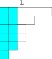
   Figure 7.1: The first two columns of the partition $\lambda$ are highlighted.

2. If $n$ is odd, then each polynomial irreducible representation is isomorphic to $V_{[\lambda]}$ for some $\lambda$.

Let

$$V_{[\lambda]}\otimes V_{[\mu]}=\otimes_{\gamma}d_{\lambda,\mu}^{\gamma}V_{[\gamma]}$$

be the decomposition of $V_{[\lambda]}\otimes V_{[\mu]}$ into irreducibles. Here $d_{\lambda,\mu}^{\gamma}$ is called the Littlewood-Richardson coefficient of type B. The types of various connected reductive groups are defined as follows:

• $GL_{n}(\mathbb{C})$: type A

• $O_{n}(\mathbb{C})$, $n$ odd: type B

• $Sp_{n}(\mathbb{C})$: type C

• $O_{n}(\mathbb{C})$, $n$ even: type D

The Littlewood-Richardson coefficient can be defined for any type in a similar fashion.

Theorem 7.6 (Generalized Littlewood-Richardson rule).

The Littlewood-Richardson coefficient $d_{\lambda,\mu}^{\gamma}\in\#P$. This also holds for any type.

Proof.

The most transparent proof of this theorem comes through the theory of quantum groups [K]; cf. Chapter 20. ∎

As in type $A$ this leads to:

Hypothesis 7.1 (PH$1$).

There exists a polytope $P_{\lambda,\mu}^{\gamma}$ of dimension polynomial in the heights of $\lambda,\mu$ and $\gamma$ such that:

1. $d_{\lambda,\mu}^{\gamma}=\varphi(P_{\lambda,\mu}^{\gamma})$, the number of integer points in $P_{\lambda,\mu}^{\gamma}$, and

2. $\widetilde{d}_{\lambda,\mu}^{\gamma}(k)=d_{k\lambda,k\mu}^{k\gamma}$ is the Ehrhart quasipolynomial of $P_{\lambda,\mu}^{\gamma}$.

There are several choices for such polytopes; e.g. the BZ-polytope [BZ].

Theorem 7.7 (De Loera, McAllister [DM2]).

The stretching function $\widetilde{d}_{\lambda,\mu}^{\gamma}(k)$ is a quasipolynomial of degree at most $2$; so also for types $C$ and $D$.

A verbatim translation of the saturation property fails here [Z]): there exist $\lambda,\mu$ and $\gamma$ such that $d_{2\lambda,2\mu}^{2\gamma}\neq 0$ but $d_{\lambda,\mu}^{\gamma}=0$. Therefore we change the definition of saturation:

Definition 7.4.

Given a quasipolynomial $f(k)=(f_{i})$, $index(f)$ is the smallest $i$ such that $f_{i}(k)$ is not an identically zero polynomial. If $f(k)$ is identically zero, $index(f)=0$.

Definition 7.5.

A quasipolynomial $f(k)$ is saturated if $f(index(f))\neq 0$. In particular, if $index(f)=1$, then $f(k)$ is saturated if $f(1)\neq 0$.

A positive quasi-polynomial is clearly saturated.

Positivity Hypothesis 2 (PH2) [DM2]: The stretching quasipolyomial $\widetilde{d}_{\lambda,\mu}^{\gamma}(k)$ is positive.

There is considerable evidence for this.

Saturation Hypothesis (SH): The stretching quasipolynomial $\widetilde{d}_{\lambda,\mu}^{\gamma}(k)$ is saturated.

PH2 implies SH.

Theorem 7.8.

[GCT5] Assuming SH (or PH$2$), positivity of the Littlewood-Richardson coefficient $d_{\lambda,\mu}^{\gamma}$ of type $B$ can be decided in $poly({\langle{\lambda}\rangle},{\langle{\mu}\rangle},{\langle{\gamma}\rangle})$ time.

This is also true for all types.

Proof.

next class. ∎

Chapter 8 Deciding nonvanishing of Littlewood-Richardson coefficients for $O_{n}(\mathbb{C})$

Scribe: Hariharan Narayanan

Goal: A polynomial time algorithm for deciding nonvanishing of Littlewood-Richardson coefficients for the orthogonal group assuming SH.

Reference: [GCT5]

Let $d_{\lambda,\mu}^{\nu}$ denote the Littlewood-Richardson coefficient of type $B$ (i.e. for the orthogonal group $O_{n}(\mathbb{C})$, $n$ odd) as defined in the earlier lecture. In this lecture we describe a polynomial time algorithm for deciding nonvanishing of $d_{\lambda,\mu}^{\nu}$ assuming the following positivity hypothesis PH2. Similar result also holds for all types, though we shall only concentrate on type B in this lecture.

Let $\tilde{d}_{\lambda,\mu}^{\nu}(k)=d_{k\lambda,k\mu}^{k\nu}$ denote the associated stretching function. It is known to be a quasi-polynomial of period at most two [DM2]. This means there are polynomials $f_{1}(k)$ and $f_{2}(k)$ such that

$$d_{k\lambda,k\mu}^{k\nu}=\left\{\begin{array}[]{ll}f_{1}(k),&\hbox{if k is odd;}\\ f_{2}(k),&\hbox{if k is even.}\end{array}\right.$$

Positivity Hypothesis (PH2) [DM2]: The stretching quasi-polynomial $\tilde{d}_{\lambda,\mu}^{\nu}(k)$ is positive. This means the coefficients of $f_{1}$ and $f_{2}$ are all non-negative.

The main result in this lecture is:

Theorem 8.1.

[GCT5] If PH2 holds, then the problem of deciding the positivity (nonvanishing) of $d_{\lambda\mu}^{\nu}$ belongs to $P$. That is, this problem can be solved in time polynomial in the bitlengths of $\lambda,\mu$ and $\nu$.

We need a few lemmas for the proof.

Lemma 8.1.

If PH2 holds, the following are equivalent:

1. $d_{\lambda\mu}^{\nu}\geq 1$.

2. There exists an odd integer $k$ such that $d_{k\lambda\,k\mu}^{k\nu}\geq 1$.

Proof: Clearly $(1)$ implies $(2)$. By PH2, there exists a polynomial $f_{1}$ with non-negative coefficients such that

$$\forall\text{ odd }k,\,f_{1}(k)=d_{k\lambda\,k\mu}^{k\nu}.$$

Suppose that for some odd $k$, $d_{k\lambda\,k\mu}^{k\nu}\geq 1.$ Then $f_{1}(k)\geq 1$. Therefore $f_{1}$ has at least one non-zero coefficient. Since all coefficients of $f_{1}$ are nonnegative, $d_{\lambda\mu}^{\nu}=f_{1}(1)>0$. Since $d_{\lambda\mu}^{\nu}$ is an integer, $(1)$ follows. $\Box$

Definition 8.1.

Let $\mathbb{Z}_{<2>}$ be the subring of  $\mathbb{Q}$ obtained by localizing $\mathbb{Z}$ at $2$:

$$\mathbb{Z}_{<2>}:=\left\{\frac{p}{q}\mid p,\frac{q-1}{2}\in\mathbb{Z}\right\}.$$

This ring consists of all fractions whose denominators are odd.

Lemma 8.2.

Let $P\in\mathbb{R}^{d}$ be a convex polytope specified by $Ax\leq B$, $x_{i}\geq 0$ for all $i$, where $A$ and $B$ are integral. Let ${\mathrm{Aff}}(P)$ denote its affine span. The following are equivalent:

1. $P$ contains a point in $\mathbb{Z}_{<2>}^{d}$.

2. ${\mathrm{Aff}}(P)$ contains a point in $\mathbb{Z}_{<2>}^{d}$.

Proof: Since $P\subseteq{\mathrm{Aff}}(P)$, $(1)$ implies $(2)$. Now suppose $(2)$ holds. We have to show $(1)$. Let $z\in{\mathbb{Z}_{<2>}^{d}}\cap{\mathrm{Aff}}(P)$.

First, consider the case when ${\mathrm{Aff}}(P)$ is one dimensional. In this case, $P$ is the line segment joining two points $x$ and $y$ in $\mathbb{Q}^{d}$. The point $z$ can be expressed as an affine linear combination, $z=ax+(1-a)y$ for some $a\in\mathbb{Q}$. There exists $q\in\mathbb{Z}\text{ such that }qx\in{\mathbb{Z}_{<2>}^{d}}\text{ and }qy\in{\mathbb{Z}_{<2>}^{d}}.$ Note that

$$\{z+\lambda(qx-qy)\mid\lambda\in{\mathbb{Z}_{<2>}}\}\subseteq{\mathrm{Aff}}(P)\cap{\mathbb{Z}_{<2>}^{d}}.$$

Since ${\mathbb{Z}_{<2>}}$ is a dense subset of $\mathbb{Q}$, the l.h.s. and hence the r.h.s. is a dense subset of ${\mathrm{Aff}}(P)$. Consequently, $P\cap{\mathbb{Z}_{<2>}^{d}}\neq\emptyset$.

Now consider the general case. Let $u$ be any point in the interior of $P$ with rational coordinates, and $L$ the line through $u$ and $z$. By restricting to $L$, the lemma reduces to the preceding one dimensional case. $\Box$

Lemma 8.3.

Let

$$P=\left\{x\mid Ax\leq B,(\forall i)x_{i}\geq 0\right\}\subseteq\mathbb{R}^{d}$$

be a convex polytope where $A$ and $B$ are integral. Then, it is possible to determine in polynomial time whether or not ${\mathrm{Aff}}(P)\cap{\mathbb{Z}_{<2>}^{d}}=\emptyset$.

Proof: Using Linear Programming [Kha79, Kar84], a presentation of the form $Cx=D$ can be obtained for ${\mathrm{Aff}}(P)$ in polynomial time, where $C$ is an integer matrix and $D$ is a vector with integer coordinates. We may assume that $C$ is square since this can be achieved by padding it with $0$’s if necessary, and extending $D$. The Smith Normal Form over $\mathbb{Z}$ of $C$ is a matrix $S$ such that $C=USV$ where $U$ and $V$ are unimodular and $S$ has the form

$$\left(\begin{array}[]{cccc}s_{11}&0&\dots&0\\ 0&s_{22}&\dots&0\\ \vdots&\vdots&\ddots&0\\ 0&0&\dots&s_{dd}\\ \end{array}\right)$$

where for $1\leq i\leq d-1$, $s_{ii}$ divides $s_{i+1\,i+1}$. It can be computed in polynomial time [KB79]. The question now reduces to whether $USVx=D$ has a solution $x\in{\mathbb{Z}_{<2>}^{d}}$. Since $V$ is unimodular, its inverse has integer entries too, and $y:=Vx\in{\mathbb{Z}_{<2>}^{d}}\Leftrightarrow x\in{\mathbb{Z}_{<2>}^{d}}$. This is equivalent to whether $Sy=U^{-1}D$ has a solution $y\in{\mathbb{Z}_{<2>}^{d}}$. Since $S$ is diagonal, this can be answered in polynomial time simply by checking each coordinate. $\Box$

Proof of Theorem 8.1: By [BZ], there exists a polytope $P=P_{\lambda,\mu}^{\nu}$ such that the Littlewood-Richardson coefficient $d_{\lambda\mu}^{\nu}$ is equal to the number of integer points in $P$. This polytope is such that the number of integer points in the dilated polytope $kP$ is $d_{k\lambda\,k\mu}^{k\nu}$. Assuming PH2, we know from Lemma 8.1 that

$$P\cap\mathbb{Z}^{d}\neq\emptyset\Leftrightarrow(\exists\text{ odd }k),kP\cap\mathbb{Z}^{d}\neq\emptyset.$$

The latter is equivalent to

$$P\cap{\mathbb{Z}_{<2>}^{d}}\neq\emptyset.$$

The theorem now follows from Lemma 8.2 and Lemma 8.3. $\Box$

In combinatorial optimization, LP works if the polytope is integral. In our setting, this is not necessarily the case [DM1]: the denominators of the coordinates of the vertices of $P$ can be $\Omega(l)$, where $l$ is the total height of $\lambda,\mu$ and $\nu$. LP works here nevertheless because of PH2; it can be checked that SH is also sufficient.

Chapter 9 The plethysm problem

Scribe: Joshua A. Grochow

Goal: In this lecture we describe the general plethysm problem, state analogous positivity and saturation hypotheses for it, and state the results from GCT 6 which imply a polynomial time algorithm for deciding positivity of a plethysm constant assuming these hypotheses.

Reference: [GCT6]

Recall

Recall that a function $f(k)$ is quasipolynomial if there are functions $f_{i}(k)$ for $i=1,\dots,\ell$ such that $f(k)=f_{i}(k)$ whenever $k\equiv i\mbox{ mod }\ell$. The number $\ell$ is then the period of $f$. The index of $f$ is the least $i$ such that $f_{i}(k)$ is not identically zero. If $f$ is identically zero, then the index of $f$ is zero by convention. We say $f$ is positive if all the coefficients of each $f_{i}(k)$ are nonnegative. We say $f$ is saturated if $f(\mbox{index}(f))\neq 0$. If $f$ is positive, then it is saturated.

Given any function $f(k)$, we associate to it the rational series $F(t)=\sum_{k\geq 0}f(k)t^{k}$.

Proposition 9.1.

[S] The following are equivalent:

1. $f(k)$ is a quasipolynomial of period $\ell$.

2. $F(t)$ is a rational function of the form $\frac{A(t)}{B(t)}$ where $\deg A<\deg B$ and every root of $B(t)$ is an $\ell$-th root of unity.

9.1 Littlewood-Richardson Problem [GCT 3,5]

Let $G=GL_{n}(\mathbb{C})$ and $c_{\alpha,\beta}^{\gamma}$ the Littlewood-Richardson coefficient – i.e. the multiplicity of the Weyl module $V_{\gamma}$ in $V_{\alpha}\otimes V_{\beta}$. We saw that the positivity of $c_{\alpha,\beta}^{\gamma}$ can be decided in $poly({\langle{\alpha}\rangle},{\langle{\beta}\rangle},{\langle{\gamma}\rangle})$ time, where ${\langle{\cdot}\rangle}$ denotes the bit-length. Furthermore, we saw that the stretching function $\widetilde{c}_{\alpha,\beta}^{\gamma}(k)=c_{k\alpha,k\beta}^{k\gamma}$ is a polynomial, and the analogous stretching function for type $B$ is a quasipolynomial of period at most 2.

9.2 Kronecker Problem [GCT 4,6]

Now we study the analogous problem for the representations of the symmetric group (the Specht modules), called the Kronecker problem.

Let $S_{\alpha}$ be the Specht module of the symmetric group $S_{m}$ associated to the partition $\alpha$. Define the Kronecker coefficient $\kappa_{\lambda,\mu}^{\pi}$ to be the multiplicity of $S_{\pi}$ in $S_{\lambda}\otimes S_{\mu}$ (considered as an $S_{m}$-module via the diagonal action). In other words, write $S_{\lambda}\otimes S_{\mu}=\bigoplus_{\pi}\kappa_{\lambda,\mu}^{\pi}S_{\pi}$. We have $\kappa_{\lambda,\mu}^{\pi}=(\chi_{\lambda}\chi_{\mu},\chi_{\pi})$, where $\chi_{\lambda}$ denotes the character of $S_{\lambda}$. By the Frobenius character formula, this can be computed in PSPACE. More strongly, analogous to the Littlewood-Richardson problem:

Conjecture 9.1.

[GCT4, GCT6] The Kronecker coefficient $\kappa_{\lambda,\mu}^{\pi}\in\mbox{{\# P}}$. In other words, there is a positive $\#P$-formula for $\kappa_{\lambda,\mu}^{\pi}$.

This is a fundamental problem in representation theory. More concretely, it can be phrased as asking for a set of combinatorial objects $I$ and a characteristic function $\chi:\{I\}\to\{0,1\}$ such that $\chi\in\mbox{{FP}}$ and $\kappa_{\lambda,\mu}^{\pi}=\sum_{I}\chi(I)$. Continuing our analogy:

Conjecture 9.2.

[GCT6] The problem of deciding positivity of $\kappa_{\lambda,\mu}^{\pi}$ belongs to P.

Theorem 9.1.

[GCT6] The stretching function $\widetilde{\kappa}_{\lambda,\mu}^{\pi}(k)=\kappa_{k\lambda,k\mu}^{k\pi}$ is a quasipolynomial.

Note that $\kappa_{k\lambda,k\mu}^{k\pi}$ is a Kronecker coefficient for $S_{km}$.

There is also a dual definition of the Kronecker coefficients. Namely, consider the embedding

$$H=GL_{n}(\mathbb{C})\times GL_{n}(\mathbb{C})\hookrightarrow G=GL(\mathbb{C}^{n}\otimes\mathbb{C}^{n}),$$

where $(g,h)(v\otimes w)=(gv\otimes hw)$. Then

Proposition 9.2.

[FH] The Kronecker coefficient $\kappa_{\lambda,\mu}^{\pi}$ is the multiplicity of the tensor product of Weyl modules $V_{\lambda}(GL_{n}(\mathbb{C}))\otimes V_{\mu}(GL_{n}(\mathbb{C}))$ (this is an irreducible $H$-module) in the Weyl module $V_{\pi}(G)$ considered as an $H$-module via the embedding above.

9.3 Plethysm Problem [GCT 6,7]

Next we consider the more general plethysm problem.

Let $H=GL_{n}(\mathbb{C})$, $V=V_{\mu}(H)$ the Weyl module of $H$ corresponding to a partition $\mu$, and $\rho:H\to G=GL(V)$ the corresponding representation map. Then the Weyl module $V_{\lambda}(G)$ of $G$ for a given partition $\lambda$ can be considered an $H$-module via the map $\rho$. By complete reducibility, we may decompose this $H$-representation as

$$V_{\lambda}(G)=\bigoplus_{\pi}a_{\lambda,\mu}^{\pi}V_{\pi}(H).$$

The coefficients $a_{\lambda,\mu}^{\pi}$ are known as plethsym constants (this definition can easily be generalized to any reductive group $H$). The Kronecker coefficient is a special case of the plethsym constant [Ki].

Theorem 9.2 (GCT 6).

The plethysm constant $a_{\lambda,\mu}^{\pi}\in\mbox{PSPACE}$.

This is based on a parallel algorithm to compute the plethysm constant using Weyl’s character formula. Continuing in our previous trend:

Conjecture 9.3.

[GCT6] $a_{\lambda,\mu}^{\pi}\in\mbox{{\# P}}$ and the problem of deciding positivity of $a_{\lambda,\mu}^{\pi}$ belongs to P.

For the stretching function, we need to be a bit careful. Define $\widetilde{a}_{\lambda,\mu}^{\pi}=a_{k\lambda,\mu}^{k\pi}$. Here the subscript $\mu$ is not stretched, since that would change $G$, while stretching $\lambda$ and $\pi$ only alters the representations of $G$.

As in the beginning of the lecture, we can associate a function $A_{\lambda,\mu}^{\pi}(t)=\sum_{k\geq 0}\widetilde{a}_{\lambda,\mu}^{\pi}(k)t^{k}$ to the plethysm constant. Kirillov conjectured that $A_{\lambda,\mu}^{\pi}(t)$ is rational. In view of Proposition 9.1, this follows from the following stronger result:

Theorem 9.3 (GCT 6).

The stretching function $\widetilde{a}_{\lambda,\mu}^{\pi}(k)$ is a quasipolynomial.

This is the main result of GCT 6, which in some sense allows GCT to go forward. Without it, there would be little hope for proving that the positivity of plethysm constants can be decided in polynomial time. Its proof is essentially algebro-geometric. The basic idea is to show that the stretching function is the Hilbert function of some algebraic variety with nice (i.e. “rational”) singularities. Similar results are shown for the stretching functions in the algebro-geometric problems arising in GCT.

The main complexity-theoretic result in [GCT6] shows that, under the following positivity and saturation hypotheses (for which there is much experimental evidence), the positivity of the plethysm constants can indeed be decided in polynomial time (cf. Conjecture 9.3).

The first positivity hypothesis is suggested by Theorem 9.3: since the stretching function is a quasipolynomial, we may suspect that it is captured by some polytope:

Positivity Hypothesis 1 (PH1). There exists a polytope $P=P_{\lambda,\mu}^{\pi}$ such that:

1. $a_{\lambda,\mu}^{\pi}=\varphi(P)$, where $\varphi$ denotes the number of integer points inside the polytope,

2. The stretching quasipolynomial (cf. Thm. 9.3) $\widetilde{a}_{\lambda,\mu}^{\pi}(k)$ is equal to the Ehrhart quasipolynomial $f_{P}(k)$ of $P$,

3. The dimension of $P$ is polynomial in ${\langle{\lambda}\rangle},{\langle{\mu}\rangle}$, and ${\langle{\pi}\rangle}$,

4. the membership in $P_{\lambda,\mu}^{\pi}$ can be decided in $\mbox{poly}({\langle{\lambda}\rangle},{\langle{\mu}\rangle},{\langle{\pi}\rangle})$ time, and there is a polynomial time separation oracle [GLS] for $P$.

Here (4) does not imply that the polytope $P$ has only polynomially many constraints. In fact, in the plethysm problem there may be a super-polynomial number of constraints.

Positivity Hypothesis 2 (PH2). The stretching quasipolynomial $\widetilde{a}_{\lambda,\mu}^{\pi}(k)$ is positive.

This implies:

Saturation Hypothesis (SH). The stretching quasipolynomial is saturated.

Theorem 9.3 is essential to state these hypotheses, since positivity and saturation are properties that only apply to quasipolynomials. Evidence for PH1, PH2, and SH can be found in GCT 6.

Theorem 9.4.

[GCT6] Assuming PH1 and SH (or PH2), positivity of the plethysm constant $a_{\lambda,\mu}^{\pi}$ can be decided in $\mbox{poly}({\langle{\lambda}\rangle},{\langle{\mu}\rangle},{\langle{\pi}\rangle})$ time.

This follows from the polynomial time algorithm for saturated integer programming described in the next class. As with Theorem 9.3, this also holds for more general problems in algebraic geometry.

Chapter 10 Saturated and positive integer programming

Scribe: Sourav Chakraborty

Goal : A polynomial time algorithm for saturated integer programming and its application to the plethysm problem.

Reference: [GCT6]

Notation : In this class we denote by $\langle a\rangle$ the bit-length of the $a$.

10.1 Saturated, positive integer programming

Let $Ax\leq b$ be a set of inequalities. The number of constraints can be exponential. Let $P\subset\mathbb{R}^{n}$ be the polytope defined by these inequalities. The bit length of P is defined to be $\langle P\rangle=n+\psi$, where $\psi$ is the maximum bit-length of a constraint in the set of inequalities. We assume that P is given by a separating oracle. This means membership in $P$ can be decided in poly$(\langle P\rangle)$ time, and if $x\not\in P$ then a separating hyperplane is given as a proof as in [GLS].

Let $f_{P}(k)$ be the Ehrhart quasi-polynomial of P. Quasi-polynomiality means there exist polynomials $f_{i}(k)$, $1\leq i\leq l$, $l$ the period, so that $f_{P}(k)=f_{i}(k)$ if $k=i$ modulo $l$. Then

$$\mbox{Index($f_{P}$) = min}\{i|f_{i}(k)\mbox{not identically $0$ as a polynomial}\}$$

The integer programming problem is called positive if $f_{P}(k)$ is positive whenever $P$ is non-empty, and saturated if $f_{P}(k)$ is saturated whenever $P$ is non-empty.

Theorem 10.1 (GCT6).

1. Index$(f_{P})$ can be computed in time polynomial in the bit length $\langle P\rangle$ of $P$ assuming that the separation oracle works in poly-$\langle P\rangle$-time.

2. Saturated and hence positive integer programming problem can be solved in poly-$\langle P\rangle$-time.

The second statement follow from the first.

Proof.

Let $Aff(P)$ denote the affine span of P. By [GLS] we can compute the specifications $Cx=d$, $C$ and $d$ integral, of $Aff(P)$ in poly$(\langle P\rangle)$ time. Without loss of generality, by padding, we can assume that $C$ is square. By [KB79] we find the Smith-normal form of $C$ in polynomial time. Let it be $\bar{C}$. So,

$$\bar{C}=ACB$$

where $A$ and $B$ are unimodular, and $\bar{C}$ is a diagonal matrix, where the diagonal entries $c_{1},c_{2},\dots$ are such that with $c_{i}|c_{i+1}$.

Clearly $Cx=d$ iff $\bar{C}z=\bar{d}$ where $z=B^{-1}x$ and $\bar{d}=Ad$.

So all equations here are of form

$$\bar{c_{i}}z_{i}=d_{i}$$ (10.1)

Without loss of generality we can assume that $c_{i}$ and $d_{i}$ are relatively prime. Let $\tilde{c}=lcm(c_{i})$.

Claim 10.1.

$Index(f_{P})=\tilde{c}$.

From this claim the theorem clearly follows.

Proof of the claim.

Let $f_{P}(t)=\sum_{k\geq 0}f_{P}(k)t^{k}$ be the Ehrhart Series of $P$.

Now $kP$ will not have an integer point unless $\tilde{c}$ divides $k$ because of (10.1).

Hence $f_{P}(t)=f_{\bar{P}}(t^{\tilde{c}})$ where $\bar{P}$ is the stretched polytope $\tilde{c}P$ and $f_{\bar{P}}(s)$ is the Ehrhart series of $\bar{P}$. From this it follows that

$$Index(f_{P})=\tilde{c}Index(f_{\bar{P}})$$

Now we show that $Index(f_{\bar{P}})=1$.

The equations of $\bar{P}$ are of the form

$$z_{i}=\frac{\tilde{c}}{c_{i}}d_{i}$$

where each $\frac{\tilde{c}}{c_{i}}$ is an integer. Therefore without loss of generality we can ignore these equations and assume the $\bar{P}$ is full dimensional.

Then it suffices to show that $\bar{P}$ contains a rational point whose denominators are all 1 modulo $\ell(\bar{P})$, the period of the quasi-polynomial $f_{\bar{P}}(s)$.

This follows from a simple density argument that we saw earlier (cf. the proof of Lemma 8.2).

From this the claim follows. ∎

∎

10.2 Application to the plethysm problem

Now we can prove the result stated in the last class:

Theorem 10.2.

Assuming PH1 and SH, positivity of the plethysm constant $a^{\pi}_{\lambda,\mu}$ can be decided in time polynomial in $\langle\lambda\rangle,\langle\mu\rangle$ and $\langle\pi\rangle$.

Proof.

Let $P=P_{\lambda,\mu}^{\pi}$ be the polytope as in PH1 such that $a^{\pi}_{\lambda,\mu}$ is the number of integer points in $P$. The goal is to decide if $P$ contains an integer point. This integer programming problem is saturated because of SH. Hence the result follows from Theorem 10.1. ∎

Chapter 11 Basic algebraic geometry

Scribe: Paolo Codenotti

Goal: So far we have focussed on purely representation-theoretic aspects of GCT. Now we have to bring in algebraic geometry. In this lecture we review the basic definitions and results in algebraic geometry that will be needed for this purpose. The proofs will be omitted or only sketched. For details, see the books by Mumford [Mm] and Fulton [F].

11.1 Algebraic geometry definitions

Let $V=\mathbb{C}^{n}$, and $v_{1},\dots,v_{n}$ the coordinates of $V$.

Definition 11.1.

• $Y$ is an affine algebraic set in $V$ if $Y$ is the set of simultaneous zeros of a set of polynomials in $v_{i}$’s.

• An algebraic set that cannot be written as the union of two proper algebraic sets $Y_{1}$ and $Y_{2}$ is called irreducible.

• An irreducible affine algebraic set is called an affine variety.

• The ideal of an affine algebraic set $Y$ is $I(Y)$, the set of all polynomials that vanish on $Y$.

For example, $Y=(v_{1}-v_{2}^{2}+v_{3},v_{3}^{2}-v_{2}+4v_{1})$ is an irreducible affine algebraic set (and therefore an affine variety).

Theorem 11.1 (Hilbert).

$I(Y)$ is finitely generated, i.e. there exist polynomials $g_{1},\dots,g_{k}$ that generate $I(Y)$. This means every $f\in I(Y)$ can be written as $f=\sum f_{i}g_{i}$ for some polynomials $f_{i}$.

Let $\mathbb{C}[V]$, the coordinate ring of $V$, be the ring of polynomials over the variables $v_{1},\dots,v_{n}$. The coordinate ring of $Y$ is defined to be $\mathbb{C}[Y]=\mathbb{C}[V]/I(Y)$. It is the set of polynomial functions over $Y$.

Definition 11.2.

• $P(V)$ is the projective space associated with $V$, i.e. the set of lines through the origin in $V$.

• $V$ is called the cone of $P(V)$.

• $\mathbb{C}[V]$ is called the homogeneous coordinate ring of $P(V)$.

• $Y\subseteq P(V)$ is a projective algebraic set if it is the set of simultaneous zeros of a set of homogeneous forms (polynomials) in the variables $v_{1},\dots,v_{n}$. It is necessary that the polynomials be homogeneous because a point in $P(V)$ is a line in $V$.

• A projective algebraic set $Y$ is irreducible if it can not be expressed as the union of two proper algebraic sets in $P(V)$.

• An irreducible projective algebraic set is called a projective variety.

Let $Y\subseteq P(V)$ be a projective variety, and define $I(Y)$, the ideal of $Y$ to be the set of all homogeneous forms that vanish on $Y$. Hilbert’s result implies that $I(Y)$ is finitely generated.

Definition 11.3.

The cone $C(Y)\subseteq V$ of a projective variety $Y\subseteq P(V)$ is defined to be the set of all points on the lines in $Y$.

Definition 11.4.

We define the homogeneous coordinate ring of $Y$ as $R(Y)=\mathbb{C}[V]/I(Y)$, the set of homogeneous polynomial forms on the cone of $Y$.

Definition 11.5.

A Zariski open subset of $Y$ is the complement of a projective algebraic subset of $Y$. It is called a quasi-projective variety.

Let $G=GL_{n}(\mathbb{C})$, and $V$ a finite dimensional representation of $G$. Then $\mathbb{C}[V]$ is a $G$-module, with the action of $\sigma\in G$ defined by:

$$(\sigma\cdot f)(v)=f(\sigma^{-1}v),\ v\in V.$$

Definition 11.6.

Let $Y\subseteq P(V)$ be a projective variety with ideal $I(Y)$. We say that $Y$ is a $G$-variety if $I(Y)$ is a $G$-module, i.e., $I(Y)$ is a $G$-submodule of $\mathbb{C}[V]$.

If $Y$ is a projective variety, then $R(Y)=\mathbb{C}[V]/I(Y)$ is also a $G$-module. Therefore $Y$ is $G$-invariant, i.e.

$$y\in Y\Rightarrow\sigma y\in Y,\ \forall\sigma\in G.$$

The algebraic geometry of $G$-varieties is called geometric invariant theory (GIT).

11.2 Orbit closures

We now define special classes of $G$-varieties called orbit closures. Let $v\in P(V)$ be a point, and $Gv$ the orbit of $v$:

$$Gv=\{gv|g\in G\}.$$

Let the stabilizer of $v$ be

$$H=G_{v}=\{g\in G|gv=v\}.$$

The orbit $Gv$ is isomorphic to the space $G/H$ of cosets, called the homogeneous space. This is a very special kind of algebraic variety.

Definition 11.7.

The orbit closure of $v$ is defined by:

$$\Delta_{V}[v]=\overline{Gv}\subseteq P(V).$$

Here $\overline{Gv}$ is the closure of the orbit $Gv$ in the complex topology on $P(V)$ (see figure 11.1).

Figure 11.1: The limit points of $Gv$ in $\Delta_{V}[v]$ can be horrendous.

A basic fact of algebraic geometry:

Theorem 11.2.

The orbit closure $\Delta_{V}[v]$ is a projective $G$-variety

It is also called an almost homogeneous space.

Let $I_{V}[v]$ be the ideal of $\Delta_{V}[v]$, and $R_{V}[v]$ the homogeneous coordinate ring of $\Delta_{V}[v]$. The algebraic geometry of general orbit closures is hopeless, since the closures can be horrendous (see figure 11.1). Fortunately we shall only be interested in very special kinds of orbit closures with good algebraic geometry.

We now define the simplest kind of orbit closure, which is obtained when the orbit itself is closed. Let $V_{\lambda}$ be an irreducible Weyl module of $GL_{n}(\mathbb{C})$, where $\lambda=(\lambda_{1}\geq\lambda_{2}\geq\dots\geq\lambda_{n}\geq 0)$ is a partition. Let $v_{\lambda}$ be the highest weight point in $P(V_{\lambda})$, i.e., the point corresponding to the highest weight vector in $V_{\lambda}$. This means $bv_{\lambda}=v_{\lambda}$ for all $b\in B$, where $B\subseteq GL_{\mathbf{n}}(C)$ is the Borel subgroup of lower triangular matrices. Recall that the highest weight vector is unique.

Consider the orbit $Gv_{\lambda}$ of $v_{\lambda}$. Basic fact:

Proposition 11.1.

The orbit $Gv_{\lambda}$ is already closed in $P(V)$.

It can be shown that the stabilizer $P_{\lambda}=G_{v_{\lambda}}$ is a group of block lower triangular matrices, where the block lengths only depend on $\lambda$ (see figure 11.2). Such subgroups of $GL_{n}(\mathbb{C})$ are called parabolic subgroups, and will be denoted by $P$. Clearly $Gv_{\lambda}\cong G/P_{\lambda}=G/P$.

Figure 11.2: The parabolic subgroup of block lower triangular matrices. The sizes $m_{i}$ only depend on $\lambda$.

11.3 Grassmanians

The simplest examples of $G/P$ are Grassmanians.

Definition 11.8.

Let $G=Gl_{n}(\mathbb{C})$, and $V=\mathbb{C}^{n}$. The Grassmanian $Gr_{d}^{n}$ is the space of $d$-dimensional subspaces (containing the origin) of $V$.

Examples:

1. $Gr_{1}^{2}$ is the set of lines in $\mathbb{C}^{2}$ (see figure 11.3).

2. More generally, $P(V)=Gr_{1}^{n}$.

Figure 11.3: $Gr_{1}^{2}$ is the set of lines in $\mathbb{C}^{2}$.

Proposition 11.2.

The Grassmanian $Gr_{d}^{n}$ is a projective variety (just like $P(V)=Gr_{1}^{n}$).

It is easy to see that $Gr_{d}^{n}$ is closed (since the limit of a sequence of $d$-dimensional subspaces of $V$ is a $d$-dimensional subspace). Hence this follows from:

Proposition 11.3.

Let $\lambda=(1,\ldots,1)$ be the partition of $d$, whose all parts are $1$. Then $Gr_{d}^{n}\cong Gv_{\lambda}\subseteq P(V_{\lambda})$.

Proof.

For the given $\lambda$, $V_{\lambda}$ can be identified with the $d^{\textrm{th}}$ wedge product

$$\Lambda^{d}(V)=\textrm{span}\{(v_{i_{1}}\wedge\dots\wedge v_{i_{d}})|i_{1},\dots,i_{d}\ \textrm{are distinct}\}\subseteq V\otimes\dots\otimes V\ (\textrm{d times}),$$

where

$$(v_{i_{1}}\wedge\dots\wedge v_{i_{d}})=\frac{1}{d!}\sum_{\sigma\in S_{d}}sgn(\sigma)(v_{\sigma(i_{1})}\otimes\dots\otimes v_{\sigma(i_{d})}).$$

Let $Z$ be a variable $d\times n$ matrix. Then $\mathbb{C}[Z]$ is a $G$-module: given $f\in\mathbb{C}[Z]$ and $\sigma\in GL_{n}(\mathbb{C})$, we define the action of $\sigma$ by

$$(\sigma\cdot f)(Z)=f(Z\sigma).$$

Now $\Lambda^{d}(V)$, as a $G$-module, is isomorphic to the span in $\mathbb{C}[Z]$ of all $d\times d$ minors of $Z$.

Let $A\in Gr_{d}^{n}$ be a $d$-dimensional subspace of $V$. Take any basis $\{v_{1},\dots,v_{d}\}$ of $A$. The point $v_{1}\wedge\dots\wedge v_{d}\in\Lambda^{d}(V)$ depends only on the subspace $A$, and not on the basis, since the change of basis does not change the wedge product. Let $Z_{A}$ be the $d\times n$ complex matrix whose rows are the basis vectors $v_{1},\dots,v_{d}$ of $A$. The Plucker map associates with $A$ the tuple of all $d\times d$ minors $A_{j_{1},\dots,j_{d}}$ of $Z_{A}$, where $A_{j_{1},\dots,j_{d}}$ denotes the minor of $Z_{A}$ formed by the columns $j_{1},\dots,j_{d}$. This depends only on $A$, and not on the choice of basis for $A$.

The proposition follows from:

Claim 11.1.

The Plucker map is a $G$-equivariant map from $Gr_{d}^{n}$ to $Gv_{\lambda}\subseteq P(V_{\lambda})$ and $Gr_{d}^{n}\approx Gv_{\lambda}\subseteq P(V_{\lambda})$.

Proof.

Exercise. Hint: take the usual basis, and note that the highest weight point $v_{\lambda}$ corresponds to $v_{1}\wedge\dots\wedge v_{d}$. ∎

Chapter 12 The class varieties

Scribe: Hariharan Narayanan

Goal: Associate class varieties with the complexity classes $\#P$ and $NC$ and reduce the $NC\not=P^{\#P}$ conjecture over $\mathbb{C}$ to a conjecture that the class variety for $\#P$ cannot be embedded in the class variety for $NC$.

reference: [GCT1]

The $NC\not=P^{\#P}$ conjecture over $\mathbb{C}$ says that the permanent of an $n\times n$ complex matrix $X$ cannot be expressed as a determinant of an $m\times m$ complex matrix $Y$, $m=\mbox{poly}(n)$, whose entries are (possibly nonhomogeneous) linear forms in the entries of $X$. This obviously implies the $NC\not=P^{\#P}$ conjecture over $\mathbb{Z}$, since multivariate polynomials over $\mathbb{C}^{n}$ are determined by the values that they take over the subset $\mathbb{Z}^{n}$. The conjecture over $\mathbb{Z}$ is implied by the usual $NC\not=P^{\#P}$ conjecture over a finite field $F_{p}$, $p\not=2$, and hence, has to be proved first anyway.

For this reason, we concentrate on the $NC\not=P^{\#P}$ conjecture over $\mathbb{C}$ in this lecture. The goal is to reduce this conjecture to a statement in geometric invariant theory.

12.1 Class Varieties in GCT

Towards that end, we associate with the complexity classes $\#P$ and $NC$ certain projective algebraic varieties, which we call class varieties. For this, we need a few definitions.

Let $G=GL_{\ell}(\mathbb{C})$, $V$ a finite dimensional representation of $G$. Let $P(V)$ be the associated projective space, which inherits the group action. Given a point $v\in P(V)$, let $\Delta_{V}[v]=\overline{Gv}\subseteq P(V)$ be its orbit closure. Here $\overline{Gv}$ is the closure of the orbit $Gv$ in the complex topology on $P(v)$. It is a projective $G$-variety; i.e., a projective variety with the action of $G$.

All class varieties in GCT are orbit closures (or their slight generalizations), where $v\in P(V)$ corresponds to a complete function for the class in question. The choice of the complete function is crucial, since it determines the algebraic geometry of $\Delta_{V}[v]$.

We now associate a class variety with $NC$. Let $g=det(Y)$, $Y$ an $m\times m$ variable matrix. This is a complete function for $NC$. Let $V=sym^{m}(Y)$ be the space of homogeneous forms in the entries of $Y$ of degree $m$. It is a $G$-module, $G=GL_{m^{2}}(\mathbb{C})$, with the action of $\sigma\in G$ given by:

$$\sigma:f(Y)\longmapsto f(\sigma^{-1}Y).$$

Here $\sigma^{-1}Y$ is defined thinking of $Y$ as an $m^{2}$-vector.

Let $\Delta_{V}[g]=\Delta_{V}[g,m]=\overline{Gg}$, where we think of $g$ as an element of $P(V)$. This is the class variety associated with $NC$. If $g$ is a different function instead of $det(Y)$, the algebraic geometry of $\Delta_{V}[g]$ would have been unmanageable. The main point is that the algebraic geometry of $\Delta_{V}[g]$ is nice, because of the very special nature of the determinant function.

We next associate a class variety with $\#P$. Let $h=perm(X)$, $X$ an $n\times n$ variable matrix. Let $W=sym^{n}(X)$. It is similarly an $H$-module, $H=GL_{k}(\mathbb{C})$, $k=n^{2}$. Think of $h$ as an element of $P(W)$, and let $\Delta_{W}[h]=\overline{Hh}$ be its orbit closure. It is called the class variety associated with $\#P$.

Now assume that $m>n$, and think of $X$ as a submatrix of $Y$, say the lower principal submatrix. Fix a variable entry $y$ of $Y$ outside of $X$. Define the map $\phi:W\rightarrow V$ which takes $w(x)\in W$ to $y^{m-n}w(x)\in V$. This induces a map from $P(V)$ to $P(W)$ which we call $\phi$ as well. Let $\phi(h)=f\in P(V)$ and $\Delta_{V}[f,m,n]=\overline{Gf}$ its orbit closure. It is called the extended class variety associated with $\#P$.

Proposition 12.1 (GCT 1).

1. If $h(X)\in W$ can be computed by a circuit (over $\mathbb{C}$) of depth $\leq\log^{c}(n)$, $c$ a constant, then $f=\phi(h)\in\Delta_{V}[g,m]$, for $m=O(2^{\log^{c}n})$.

2. Conversely if $f\in\Delta_{V}[g,m]$ for $m=2^{\log^{c}n}$, then $h(X)$ can be approximated infinitesimally closely by a circuit of depth $\log^{2c}m$. That is, $\forall\epsilon>0$, there exists a function $\tilde{h}(X)$ that can be computed by a circuit of depth $\leq\log^{2c}m$ such that $\|\tilde{h}-h\|<\epsilon$ in the usual norm on $P(V)$.

If the permanent $h(X)$ can be approximated infinitesimally closely by small depth circuits, then every function in $\#P$ can be approximated infinitesimally closely by small depth circuits. This is not expected. Hence:

Conjecture 12.1 (GCT 1).

Let $h(X)=perm(X)$, $X$ an $n\times n$ variable matrix. Then $f=\phi(h)\not\in\Delta_{V}[g;m]$ if $m=2^{polylog(n)}$ and $n$ is sufficiently large.

This is equivalent to:

Conjecture 12.2 (GCT 1).

The $G$-variety $\Delta_{V}[f;m,n]$ cannot be embedded as a $G$-subvariety of $\Delta_{V}[g,m]$, symbolically

$$\Delta_{V}[f;m,n]\not\hookrightarrow\Delta_{V}[g,m],$$

if $m=2^{polylog(n)}$ and $n\rightarrow\infty$.

This is the statement in geometric invariant theory (GIT) that we sought.

Chapter 13 Obstructions

Scribe: Paolo Codenotti

Goal: Define an obstruction to the embedding of the $\#P$-class variety in the $NC$-class-variety and describe why it should exist.

References: [GCT1, GCT2]

Recall

Figure 13.1: Here $Y$ is a generic $m$ by $m$ matrix, and $X$ is an $n$ by $n$ minor.

Let us first recall some definitions and results from the last class. Let $Y$ be a generic $m\times m$ variable matrix, and $X$ an $n\times n$ minor of $Y$ (see figure 13.1). Let $g=\det(Y)$, $h=\mbox{perm}(X)$, $f=\phi(h)=y^{m-n}\mbox{perm}(X)$, and $V=\mbox{Sym}^{m}[Y]$ the set of homogeneous forms of degree $m$ in the entries of $Y$. Then $V$ is a $G$-module for $G=GL(Y)=GL_{l}(\mathbb{C})$, $l=m^{2}$, with the action of $\sigma\in G$ given by

$$\sigma:f(Y)\rightarrow f(\sigma^{-1}Y),$$

where $Y$ is thought of as an $l$-vector, and $P(V)$ a $G$-variety. Let

$$\Delta_{V}[f;m,n]=\overline{Gf}\subseteq P(V),$$

and

$$\Delta_{V}[g;m]=\overline{Gg}\subseteq P(V)$$

be the class varieties associated with $\#P$ and $NC$.

13.1 Obstructions

Conjecture 13.1.

[GCT1] There does not exist an embedding $\Delta_{V}[f;m,n]\hookrightarrow\Delta_{V}[g;m]$ with $m=2^{\mbox{polylog}(n)}$, $n\rightarrow\infty$.

This implies Valiant’s conjecture that the permanent cannot be computed by circuits of polylog depth. Now we discuss how to go about proving the conjecture.

Suppose to the contrary,

$$\Delta[f;m,n]\hookrightarrow\Delta_{V}[g;m].$$ (13.1)

We denote $\Delta_{V}[f;m,n]$ by $\Delta_{V}[f]$, and $\Delta_{V}[g;m]$ by $\Delta_{V}[g]$. Let $R_{V}[g]$ be the homogeneous coordinate ring of $\Delta_{V}[g]$. The embedding (13.1) implies existence of a surjection:

$$R_{V}[f]\twoheadleftarrow R_{V}[g]$$ (13.2)

This is a basic fact from algebraic geometry. The reason is that $R_{V}[g]$ is the set of homogeneous polynomial functions on the cone $C$ of $\Delta_{V}[g]$, and any such function $\tau$ can be restricted to $\Delta_{V}[f]$ (see figure 13.2). Conversely, any polynomial function on $\Delta_{V}[f]$ can be extended to a homogeneous polynomial function on the cone $C$.

Figure 13.2: $C$ denotes the cone of $\Delta_{V}[g]$.

Let $R_{V}[f]_{d}$ and $R_{V}[g]_{d}$ be the degree $d$ components of $R_{V}[f]$ and $R_{V}[g]$. These are $G$-modules since $\Delta_{V}[f]$ and $\Delta_{V}[g]$ are $G$-varieties. The surjection (13.2) is degree preserving. So there is a surjection

$$R_{V}[f]_{d}\twoheadleftarrow R_{V}[g]_{d}$$ (13.3)

for every $d$. Since $G$ is reductive, both $R_{V}[f]_{d}$ and $R_{V}[g]_{d}$ are direct sums of irreducible $G$-modules. Hence the surjection (13.3) implies that $R_{V}[f]_{d}$ can be embedded as a $G$ submodule of $R_{V}[g]_{d}$.

Definition 13.1.

We say that a Weyl-module $S=V_{\lambda}(G)$ is an obstruction for the embedding (13.1) (or, equivalently, for the pair $(f,g)$) if $V_{\lambda}(G)$ occurs in $R_{V}[f;m,n]_{d}$, but not in $R_{V}[g;m]_{d}$, for some $d$. Here occurs means the multiplicity of $V_{\lambda}(G)$ in the decomposition of $R_{V}[f;m,n]_{d}$ is nonzero.

If an obstruction exists for given $m,n$, then the embedding (13.1) does not exist.

Conjecture 13.2 (GCT2).

An obstruction exists for the pair $(f,g)$ for all large enough $n$ if $m=2^{\textrm{polylog}(n)}$.

This implies Conjecture 13.1. In essence, this turns a nonexistence problem (of polylog depth circuit for the permanent) into an existence problem (of an obstruction).

If we replace the determinant here by any other complete function in $NC$, an obstruction need not exist. Because, as we shall see in the next lecture, the existence of an obstruction crucially depends on the exceptional nature of the class variety constructed from the determinant. The main goals of GCT in this context are:

1. understand the exceptional nature of the class varieties for $NC$ and $\#P$, and

2. use it to prove the existence of obstructions.

13.1.1 Why are the class varieties exceptional?

We now elaborate on the exceptional nature of the class varieties. Its significance for the existence of obstructions will be discussed in the next lecture.

Let $V$ be a $G$-module, $G=GL_{n}(\mathbb{C})$. Let $P(V)$ be a projective variety over $V$. Let $v\in P(V)$, and recall $\Delta_{V}[v]=\overline{Gv}$. Let $H=G_{v}$ be the stabilizer of $v$, that is, $G_{v}=\{\sigma\in G|\sigma v=v\}$.

Definition 13.2.

We say that $v$ is characterized by its stabilizer $H=G_{v}$ if $v$ is the only point in $P(V)$ such that $hv=v,\ \forall h\in H$.

If $v$ is characterized by its stabilizer, then $\Delta_{V}[v]$ is completely determined by the group triple $H\hookrightarrow G\hookrightarrow K=GL(V)$.

Definition 13.3.

The orbit closure $\Delta_{V}[v]$, when $v$ is characterized by its stabilizer, is called a group-theoretic variety.

Proposition 13.1.

[GCT1]

1. The determinant $g=\det(Y)\in P(V)$ is characterized by its stabilizer. Therefore $\Delta_{V}[g]$ is group theoretic.

2. The permanent $h=\mbox{perm}(X)\in P(W)$, where $W=\mbox{Sym}^{n}(X)$, is also characterized by its stabilizer. Therefore $\Delta_{W}[h]$ is also group theoretic.

3. Finally, $f=\phi(h)\in P(V)$ is also characterized by its stabilizer. Hence $\Delta_{V}[f]$ is also group theoretic.

Proof.

(1) It is a fact in classical representation theory that the stabilizer of $\det(Y)$ in $G=GL(Y)=GL_{m^{2}}(\mathbb{C})$ is the subgroup $G_{\det}$ that consists of linear transformations of the form $Y\rightarrow AY^{*}B$, where $Y^{*}=Y$ or $Y^{t}$, for any $A,B\in GL_{m}(\mathbb{C})$. It is clear that linear transformation of this form stabilize the determinant since:

1. $\det(AYB)=det(A)det(B)det(Y)=c\det(Y)$, where $c=\det(A)\det(B)$. Note that the constant $c$ doesn’t matter because we get the same point in the projective space.

2. $\det(Y^{*})=\det(Y)$.

It is a basic fact in classical invariant theory that $\det(Y)$ is the only point in $P(V)$ stabilized by $G_{\det}$. Furthermore, the stabilizer $G_{\det}$ is reductive, since its connected part is $(G_{\det})_{\circ}\approx GL_{m}\times GL_{m}$ with the natural embedding

$$(G_{\det})_{\circ}=GL_{m}\times GL_{m}\hookrightarrow GL(\mathbb{C}^{m}\otimes\mathbb{C}^{m})=GL_{m^{2}}(\mathbb{C})=G.$$

(2) The stabilizer of $\mbox{perm}(x)$ is the subgroup $G_{\mbox{perm}}\subseteq GL(X)=GL_{n^{2}}(\mathbb{C})$ generated by linear transformations of the form $X\rightarrow\lambda X^{*}\mu$, where $X^{*}=XorX^{t}$, and $\lambda$ and $\mu$ are diagonal (which change the permanent by a constant factor) or permutation matrices (which do not change the permanent).

Finally, the discrete component of $G_{\mbox{perm}}$ is isomorphic to $S_{2}\rtimes S_{n}\times S_{n}$, where $\rtimes$ denotes semidirect product. The continuous part is $(\mathbb{C}^{*})^{n}\times(\mathbb{C}^{*})^{n}$. So $G_{\mbox{perm}}$ is reductive.

(3) Similar.

∎

The main significance of this proposition is the following. Because $\Delta_{V}[g],\Delta_{V}[f]$, and $\Delta_{W}[h]$ are group theoretic, the algebraic geometric problems concerning these varieties can be “reduced” to problems in the theory of quantum groups. So the plan is:

1. Use the theory of quantum groups to understand the structure of the group triple associated with the algebraic variety.

2. Translate this understanding to the structure of the algebraic variety.

3. Use this to show the existence of obstructions.

Chapter 14 Group theoretic varieties

Scribe: Joshua A. Grochow

Goal: In this lecture we continue our discussion of group-theoretic varieties. We describe why obstructions should exist, and why the exceptional group-theoretic nature of the class varieties is crucial for this existence.

Recall

Let $G=GL_{n}(\mathbb{C})$, $V$ a $G$-module, and $\mathbb{P}(V)$ the associated projective space. Let $v\in\mathbb{P}(V)$ be a point characterized by its stabilizer $H=G_{v}\subset G$. In other words, $v$ is the only point in $\mathbb{P}(V)$ stabilized by $H$. Then $\Delta_{V}[v]=\overline{Gv}$ is called a group-theoretic variety because it is completely determined by the group triple

$$H\hookrightarrow G\hookrightarrow GL(V).$$

The simplest example of a group-theoretic variety is a variety of the form $G/P$ that we described in the earlier lecture. Let $V=V_{\lambda}(G)$ be a Weyl module of $G$ and $v_{\lambda}\in\mathbb{P}(V)$ the highest weight point (recall: the unique point stabilized by the Borel subgroup $B\subset G$ of lower triangular matrices). Then the stabilizer of $v_{\lambda}$ consists of block-upper triangular matrices, where the block sizes are determined by $\lambda$:

$$P_{\lambda}:=G_{v_{\lambda}}=\left(\begin{array}[]{ccc|cc|ccc}*&*&*&*&*&*&*&*\\ &*&*&*&*&*&*&*\\ &*&*&*&*&*&*&*\\ \hline\cr 0&0&0&*&*&*&*&*\\ 0&0&0&*&*&*&*&*\\ \hline\cr 0&0&0&0&0&*&*&*\\ 0&0&0&0&0&*&*&*\\ 0&0&0&0&0&*&*&*\end{array}\right)$$

The orbit $\Delta_{V}[v_{\lambda}]=Gv_{\lambda}\cong G/P_{\lambda}$ is a group-theoretic variety determined entirely by the triple

$$P_{\lambda}=G_{v_{\lambda}}\hookrightarrow G\hookrightarrow K=GL(V).$$

The group-theoretic varieties of main interest in GCT are the class varieties associated with the various complexity classes.

14.1 Representation theoretic data

The main principle guiding GCT is that the algebraic geometry of a group-theoretic variety ought to be completely determined by the representation theory of the corresponding group triple. This is a natural extension of work already pursued in mathematics by Deligne and Milne on Tannakien categories [DeM], showing that an algebraic group is completely determined by its representation theory. So the goal is to associate to a group-theoretic variety some representation-theoretic data that will analogously capture the information in the variety completely. We shall now illustrate this for the class variety for $NC$. First a few definitions.

Let $v\in\mathbb{P}(V)$ be the point as above characterized by its stabilizer $G_{v}$. This means the line $\mathbb{C}v\subseteq V$ corresponding to $v$ is a one-dimensional representation of $G_{v}$. Thus $(\mathbb{C}v)^{\otimes d}$ is a one-dimensional degree $d$ representation, i.e. the representation $\rho:G\to GL(\mathbb{C}v)\cong\mathbb{C}^{*}$ is polynomial of degree $d$ in the entries of the matrix of an element in $G$. Recall that $\mathbb{C}[V]$ is the coordinate ring of $V$, and $\mathbb{C}[V]_{d}$ is its degree $d$ homogeneous component, so $(\mathbb{C}v)^{\otimes d}\subseteq\mathbb{C}[V]_{d}$.

To each $v\in\mathbb{P}(V)$ that is characterized by its stabilizer, we associate a representation-theoretic data, which is the set of $G$-modules

$$\Pi_{v}=\bigcup_{d}\Pi_{v}(d),$$

where $\Pi_{v}(d)$ is the set of all irreducible $G$-submodules $S$ of $\mathbb{C}[V]_{d}$ whose duals $S^{*}$ do not contain a $G_{v}$-submodule isomorphic to $(\mathbb{C}v)^{\otimes d*}$ (the dual of $(\mathbb{C}v)^{\otimes d}$). The following proposition elucidates the importance of this data:

Proposition 14.1.

[GCT2] $\Pi_{v}\subseteq I_{V}[v]$ (where $I_{V}[v]$ is the ideal of the projective variety $\Delta_{V}[v]\subseteq\mathbb{P}(V)$).

Proof.

Fix $S\in\Pi_{v}(d)$. Suppose, for the sake of contradiction, that $S\nsubseteq I_{V}[v]$. Since $S\subseteq\mathbb{C}[V]$, $S$ consists of “functions” on the variety $\mathbb{P}(V)$ (actually homogeneous polynomials on $V$). The coordinate ring of $\Delta_{V}[v]$ is $\mathbb{C}[V]/I_{V}[v]$, and since $S\nsubseteq I_{V}[v]$, $S$ must not vanish identically on $\Delta_{V}[v]$. Since the orbit $Gv$ is dense in $\Delta_{V}[v]$, $S$ must not vanish identically on this single orbit $Gv$. Since $S$ is a $G$-module, if $S$ were to vanish identically on the line $\mathbb{C}v$, then it would vanish on the entire orbit $Gv$, so $S$ does not vanish identically on $\mathbb{C}v$.

Now $S$ consists of functions of degree $d$. Restrict them to the line $\mathbb{C}v$. The dual of this restriction gives an injection of $(\mathbb{C}v)^{\otimes d*}$ as a $G_{v}$-submodule of $S^{*}$, contradicting the definition of $\Pi_{v}(d)$. ∎

14.2 The second fundamental theorem

We now ask essentially the reverse question: when does the representation theoretic data $\Pi_{v}$ generate the ideal $I_{V}[v]$? For if $\Pi_{v}$ generates $I_{V}[v]$, then $\Pi_{v}$ completely captures the coordinate ring $\mathbb{C}[V]/I_{V}[v]$, and hence the variety $\Delta_{V}[v]$.

Theorem 14.1 (Second fundamental theorem of invariant theory for $G/P$).

The $G$-modules in $\Pi_{v_{\lambda}}(2)$ generate the ideal $I_{V}[v_{\lambda}]$ of the orbit $Gv_{\lambda}\cong G/P_{\lambda}$, when $V=V_{\lambda}(G)$.

This theorem justifies the main principle for $G/P$, so we can hope that similar results hold for the class varieties in GCT (though not always exactly in the same form).

Now, let $\Delta_{V}[g]$ be the class variety for NC (in other words, take $g=\det(Y)$ for a matrix $Y$ of indeterminates). Based on the main principle, we have the following conjecture, which essentially generalizes the second fundamental theorem of invariant theory for $G/P$ to the class variety for NC:

Conjecture 14.1 (GCT 2).

$\Delta_{V}[g]=X(\Pi_{g})$ where $X(\Pi_{g})$ is the zero-set of all forms in the $G$-modules contained in $\Pi_{g}$.

Theorem 14.2 (GCT 2).

A weaker version of the above conjecture holds. Specifically, assuming that the Kronecker coefficients satisfy a certain separation property, there exists a $G$-invariant (Zariski) open neighbourhood $U\subseteq P(V)$ of the orbit $Gg$ such that $X(\Pi_{g})\cap U=\Delta_{V}[g]\cap U$.

There is a notion of algebro-geometric complexity called Luna-Vust complexity which quantifies the gap between $G/P$ and class varieties. The Luna-Vust complexity of $G/P$ is 0. The Luna-Vust complexity of the NC class variety is $\Omega(\dim(Y))$. This is analogous to the difference between circuits of constant depth and circuits of superpolynomial depth. This is why the previous conjecture and theorem turn out to be far harder than the corresponding facts for $G/P$.

14.3 Why should obstructions exist?

The following proposition explains why obstructions should exist to separate NC from $P^{\#P}$.

Proposition 14.2 (GCT 2).

Let $g=\det(Y)$, $h=\mbox{perm}(X)$, $f=\phi(h)$, $n=\dim(X)$, $m=\dim(Y)$. If Conjecture 14.1 holds and the permanent cannot be approximated arbitrarily closely by circuits of poly-logarithmic depth (hardness assumption), then an obstruction for the pair $(f,g)$ exists for all large enough $n$, when $m=2^{\log^{c}n}$ for some constant $c$. Hence, under these conditions, $\mbox{{NC}}\neq\mbox{{$P^{\#P}$}}$ over $\mathbb{C}$.

This proposition may seem a bit circular at first, since it relies on a hardness assumption. But we do not plan to prove the existence of obstructions by proving the assumptions of this proposition. Rather, this proposition should be taken as evidence that obstructions exist (since we expect the hardness assumption therein to hold, given that the permanent is # P-complete), and we will develop other methods to prove their existence.

Proof.

The hardness assumption implies that $f\notin\Delta_{V}[g]$ if $m=2^{\log^{c}n}$ [GCT 1].

Conjecture 14.1 says that $X(\Pi_{g})=\Delta_{V}[g]$. So there exists an irreducible $G$-module $S\in\Pi_{g}$ such that $S$ does not vanish on $f$. So $S$ occurs in $R_{V}[f]$ as a $G$-submodule.

On the other hand, since $S\in\Pi_{g}$, $S\subseteq I_{V}[g]$ by Proposition 14.1. So $S$ does not occur in $R_{V}[g]=\mathbb{C}[V]/I_{V}[g]$. Thus $S$ is not a $G$-submodule of $R_{V}[g]$, but it is a $G$-submodule of $R_{V}[f]$, i.e., $S$ is an obstruction. ∎

Chapter 15 The flip

Scribe: Hariharan Narayanan

Goal: Describe the basic principle of GCT, called the flip, in the context of the $NC$ vs. $P^{\#P}$ problem over $\mathbb{C}$.

references: [GCTflip1, GCT1, GCT2, GCT6]

Recall

As in the previous lectures, let $g=det(Y)\in P(V)$, $Y$ an $m\times m$ variable matrix, $G=GL_{m^{2}}(\mathbb{C})$, and $\Delta_{V}(g)=\Delta_{V}[g;m]=\overline{G}g\subseteq P(V)$ the class variety for NC. Let $h=perm(X)$, $X$ an $n\times n$ variable matrix, $f=\phi(h)=y^{m-n}h\in P(V)$, and $\Delta_{V}(f)=\Delta_{V}[f;m,n]=\overline{G}f\subseteq P(V)$ the class variety for $P^{\#P}$. Let $R_{V}[f;m,n]$ denote the homogeneous coordinate ring of $\Delta_{V}[f;m,n]$, $R_{V}[g;m]$ the homogeneous coordinate ring of $\Delta_{V}[g;m]$, and $R_{V}[f;m,n]_{d}$ and $R_{V}[g;m]_{d}$ their degree $d$-components. A Weyl module $S=V_{\mathbf{\lambda}}(G)$ of $G$ is an obstruction of degree $d$ for the pair $(f,g)$ if $V_{\mathbf{\lambda}}$ occurs in $R_{V}[f;m,n]_{d}$ but not $R_{V}[g;m]_{d}$.

Conjecture 15.1.

[GCT2] An obstruction (of degree polynomial in $m$) exists if $m=2^{\text{polylog}(n)}$ as $n\rightarrow\infty$.

This implies $NC\not=P^{\#P}$ over $\mathbb{C}$.

15.1 The flip

In this lecture we describe an approach to prove the existence of such obstructions. It is based on the following complexity theoretic positivity hypothesis:

PHflip [GCTflip1]:

1. Given $n,m$ and $d$, whether an obstruction of degree $d$ for $m$ and $n$ exists can be decided in $poly(n,m,{\langle{d}\rangle})$ time, and if it exists, the label ${\mathbf{\lambda}}$ of such an obstruction can be constructed in $poly(n,m,{\langle{d}\rangle})$ time. Here ${\langle{d}\rangle}$ denotes the bitlength of $d$.

2. 1. Whether $V_{\mathbf{\lambda}}$ occurs in $R_{V}[f;m,n]_{d}$ can be decided in $poly(n,m,{\langle{d}\rangle},{\langle{{\mathbf{\lambda}}}\rangle})$ time.

   2. Whether $V_{\mathbf{\lambda}}$ occurs in $R_{V}[g;m]_{d}$ can be decided in $poly(n,m,{\langle{d}\rangle},{\langle{{\mathbf{\lambda}}}\rangle})$ time.

This suggests the following approach for proving Conjecture 15.1:

1. Find polynomial time algorithms sought in PHflip-2 for the basic decision problems (a) and (b) therein.

2. Using these find a polynomial time algorithm sought in PHflip-1 for deciding if an obstruction exists.

3. Transform (the techniques underlying) this “easy” (polynomial time) algorithm for deciding if an obstruction exists for given $n$ and $m$ into an “easy” (i.e., feasible) proof of existence of an obstruction for every $n\rightarrow\infty$ when $d$ is large enough and $m=2^{\mbox{polylog}(n)}$.

The first step here is the crux of the matter. The main results of [GCT6] say that the polynomial time algorithms for the basic decision problems as sought in PHflip-2 indeed exist assuming natural analogues of PH1 and SH (PH2) that we have seen earlier in the context of the plethysm problem. To state them, we need some definitions.

Let $S_{d}^{\mathbf{\lambda}}[f]=S_{d}^{\mathbf{\lambda}}[f;m,n]$ be the multiplicity of $V_{\mathbf{\lambda}}=V_{\mathbf{\lambda}}(G)$ in $R_{V}[f;m,n]$. The stretching function $\tilde{S}_{d}[f]=\tilde{S}_{d}^{\mathbf{\lambda}}[f;m,n]$ is defined by

$$\tilde{S}_{d}^{\mathbf{\lambda}}[f](k):=S_{kd}^{k{\mathbf{\lambda}}}[f].$$

The stretching function for $g$, $\tilde{S}^{\lambda}_{d}[g]=\tilde{S}^{\lambda}_{d}[g;m]$, is defined analogously.

The main mathematical result of [GCT6] is:

Theorem 15.1.

[GCT6] The stretching functions $\tilde{S}_{d}^{\mathbf{\lambda}}[g]$ and $\tilde{S}_{d}^{\mathbf{\lambda}}[f]$ are quasipolynomials assuming that the singularities of $\Delta_{V}[f;m,n]$ and $\Delta_{V}[g;m]$ are rational.

Here rational means “nice”; we shall not worry about the exact definition.

The main complexity-theoretic result is:

Theorem 15.2.

[GCT6] Assuming the following mathematical positivity hypothesis $PH1$ and the saturation hypothesis $SH$ (or the stronger positivity hypothesis $PH2$), PHflip-2 holds.

PH1: There exists a polytope $P=P_{d}^{\mathbf{\lambda}}[f]$ such that

1. The Ehrhart quasi-polynomial of $P$, $f_{P}(k)$, is $\tilde{S}_{d}^{\mathbf{\lambda}}[f](k)$.

2. $dim(P)=poly(n,m,{\langle{d}\rangle})$.

3. Membership in $P$ can be answered in polynomial time.

4. There is a polynomial time separation oracle [GLS] for $P$.

Similarly, there exists a polytope $Q=Q_{d}^{\mathbf{\lambda}}[g]$ such that

1. The Ehrhart quasi-polynomial of $Q$, $f_{Q}(k)$, is $\tilde{S}_{d}^{\mathbf{\lambda}}[g](k)$.

2. $dim(Q)=poly(m,{\langle{d}\rangle})$.

3. Membership in $Q$ can be answered in polynomial time.

4. There is a polynomial time separation oracle for $Q$.

PH2: The quasi-polynomials $\tilde{S}_{d}^{\mathbf{\lambda}}[g]$ and $\tilde{S}_{d}^{\mathbf{\lambda}}[f]$ are positive.

This implies:

SH: The quasi-polynomials $\tilde{S}_{d}^{\mathbf{\lambda}}[g]$ and $\tilde{S}_{d}^{\mathbf{\lambda}}[f]$ are saturated.

PH1 and SH imply that the decision problems in PHflip-2 can be transformed into saturated positive integer programming problems. Hence Theorem 15.2 follows from the polynomial time algorithm for saturated linear programming that we described in an earlier class.

The decision problems in PHflip-2 are “hyped” up versions of the plethysm problem discussed earlier. The article [GCT6] provides evidence for $PH1$ and $PH2$ for the plethysm problem. This constitutes the main evidence for PH1 and PH2 for the class varieties in view of their group-theoretic nature; cf. [GCTflip1].

The following problem is important in the context of PHflip-2:

Problem 15.1.

Understand the $G$-module structure of the homogeneous coordinate rings $R_{V}[f]_{d}$ and $R_{V}[g]_{d}$.

This is an instance of the following abstract:

Problem 15.2.

Let $X$ be a projective group-theoretic $G$-variety. Let $R=\bigoplus_{d=0}^{\infty}R_{d}$ be its homogeneous coordinate ring. Understand the $G$-module structure of $R_{d}$.

The simplest group-theoretic variety is $G/P$. For it, a solution to this abstract problem is given by the following results:

1. The Borel-Weil theorem.

2. The Second Fundamental theorem of invariant theory [SFT].

These will be covered in the next class for the simplest case of $G/P$, the Grassmanian.

Chapter 16 The Grassmanian

Scribe: Hariharan Narayanan

Goal: The Borel-Weil and the second fundamental theorem of invariant theory for the Grassmanian.

Reference: [F]

Recall

Let $V=V_{\mathbf{\lambda}}(G)$ be a Weyl module of $G=GL_{n}(\mathbb{C})$ and $v_{\mathbf{\lambda}}\in P(V)$ the point corresponding to its highest weight vector. The orbit $\Delta_{V}[v_{\mathbf{\lambda}}]:=Gv_{\mathbf{\lambda}}$, which is already closed, is of the form $G/P$, where $P$ is the parabolic stabilizer of $v_{\mathbf{\lambda}}$. When ${\mathbf{\lambda}}$ is a single column, it is called the Grassmannian.

An alternative description of the Grassmanian is as follows. Assume that $\lambda$ is a single column of length $d$. Let $Z$ be a $d\times n$ matrix of variables $z_{ij}$. Then $V=V_{\mathbf{\lambda}}(G)$ can be identified with the span of $d\times d$ minors of $Z$ with the action of $\sigma\in G$ given by:

$$\sigma:f(z)\mapsto f(z\sigma).$$

Let $Gr_{d}^{n}$ be the space of all d-dimensional subspaces of $\mathbb{C}^{n}$. Let $W$ be a $d$-dimensional subspace of $\mathbb{C}^{n}$. Let $B=B(W)$ be a basis of $W$. Construct the $d\times n$ matrix $z_{B}$, whose rows are vectors in $B$. Consider the Plücker map from $Gr_{d}^{n}$ to $P(V)$ which maps any $W\in Gr_{d}^{n}$ to the tuple of $d\times d$ minors of $Z_{B}$. Here the choice of $B=B(W)$ does not matter, since any choice gives the same point in $P(V)$. Then the image of $Gr_{d}^{n}$ is precisely the Grassmanian $Gv_{\lambda}\subseteq P(V)$.

16.1 The second fundamental theorem

Now we ask:

Question 16.1.

What is the ideal of $Gr_{d}^{n}\approx Gv_{\mathbf{\lambda}}\subseteq P(V)$?

The homogeneous coordinate ring of $P(V)$ is $\mathbb{C}[V]$. We want an explicit set of generators of this ideal in $\mathbb{C}[V]$. This is given by the second fundamental theorem of invariant theory, which we describe next.

The coordinates of $P(V)$ are in one-to-one correspondence with the $d\times d$ minors of the matrix $Z$. Let each minor of $Z$ be indexed by its columns. Thus for $1\leq i_{1}<\dots<i_{d}\leq n$, $Z_{i_{1},\dots,i_{d}}$ is a coordinate of $P(V)$ corresponding to the minor of $Z$ formed by the columns $i_{1},i_{2},\ldots$. Let $\Lambda(n,d)$ be the set of ordered $d$-tuples of $\{1,\dots,n\}$. The tuple $[i_{1},\ldots,i_{d}]$ in this set will be identified with the coordinate $Z_{i_{1},\dots,i_{d}}$ of $P(V)$. There is a bijection between the elements of $\Lambda(n,d)$ and of $\Lambda(n,n-d)$ obtained by associating complementary sets:

$$\Lambda(n,d)\ni{\mathbf{\lambda}}\leftrightsquigarrow{\mathbf{\lambda}}^{*}\in\Lambda(n,n-d).$$

We define $sgn({\mathbf{\lambda}},{\mathbf{\lambda}}^{*})$ to be the sign of the permutation that takes $[1,\dots,n]$ to $[{\mathbf{\lambda}}_{1},\dots,{\mathbf{\lambda}}_{d},{\mathbf{\lambda}}^{*}_{1},\dots,{\mathbf{\lambda}}^{*}_{n-d}]$.

Given $s\in\{1.\dots,d\}$, $\alpha\in\Lambda(n,s-1)$, $\beta\in\Lambda(n,d+1)$, and $\gamma\in\Lambda(n,d-s)$, we now define the Van der Waerden Syzygy $[[\alpha,\beta,\gamma]]$, which is an element of the degree two component $\mathbb{C}[V]_{2}$ of $\mathbb{C}[V]$, as follows:

$$\begin{array}[]{l}[[\alpha,\beta,\gamma]]=\\ \sum_{\tau\in\Lambda(d+1,s)}sgn(\tau,\tau^{*})[\alpha_{1},\dots,\alpha_{s-1},\beta_{\tau^{*}_{1}},\dots,\beta_{\tau^{*}_{d+1-s}}][\beta_{\tau_{1}},\dots,\beta_{\tau_{s}},\gamma_{1},\dots,\gamma_{d-s}].\end{array}$$

It is easy to show that this syzygy vanishes on the Grassmanian $Gr_{d}^{n}$: because it is an alternating $(d+1)$-multilinear-form, and hence has to vanish on any $d$-dimensional space $W\in Gr_{d}^{n}$. Thus it belongs to the ideal of the Grassmanian. Moreover:

Theorem 16.1 (Second fundamental theorem).

The ideal of the Grassmanian $Gr_{d}^{n}$ is generated by the Van-der-Waerden syzygies.

An alternative formulation of this result is as follows. Let $P_{\mathbf{\lambda}}\subseteq G$ be the stabilizer of $v_{\mathbf{\lambda}}$. Let $\Pi_{v_{\mathbf{\lambda}}}(2)$ be the set of irreducible $G$-submodules of $\mathbb{C}[V]_{2}$ whose duals do not contain a $P_{\mathbf{\lambda}}$-submodule isomorphic to $\mathbb{C}v_{\mathbf{\lambda}}^{\otimes 2*}$ (the dual of $\mathbb{C}v_{\mathbf{\lambda}}^{\otimes 2}$). Here $\mathbb{C}v_{\mathbf{\lambda}}$ denotes the line in $P(V)$ corresponding to $v_{\lambda}$, which is a one-dimensional representation of $P_{\mathbf{\lambda}}$ since it stabilizes $v_{\mathbf{\lambda}}\in P(V)$. It can be shown that the span of the $G$-modules in $\Pi_{v_{\mathbf{\lambda}}}(2)$ is equal to the span of the Van-der-Waerden syzygies. Hence, Theorem 16.1 is equivalent to:

Theorem 16.2 (Second Fundamental Theorem(SFT)).

The $G$-modules in $\Pi_{v_{\mathbf{\lambda}}}(2)$ generate the ideal of $Gr_{d}^{n}$.

This formulation of SFT for the Grassmanian looks very similar to the generalized conjectural SFT for the $NC$-class variety described in the earlier class. This indicates that the class varieties in GCT are “qualitatively similar” to $G/P$.

16.2 The Borel-Weil theorem

We now describe the $G$-module structure of the homogeneous coordinate ring $R$ of the Grassmannian $Gv_{\mathbf{\lambda}}\subseteq P(V)$, where ${\mathbf{\lambda}}$ is a single column of height $d$. The goal is to give an explicit basis for $R$. Let $R_{s}$ be the degree $s$ component of $R$. Corresponding to any numbering $T$ of the shape $s{\mathbf{\lambda}}$, which is a $d\times s$ rectangle, whose columns have strictly increasing elements top to bottom, we have a monomial $m_{T}=\prod_{c}Z_{c}\in\mathbb{C}[V]_{s}$, were $Z_{c}$ is the coordinate of $P(V)$ indexed by the $d$-tuple $c$, and $c$ ranges over the $s$ columns of $T$. We say that $m_{T}$ is (semi)-standard if the rows of $T$ are nondecreasing, when read left to right. It is called nonstandard otherwise.

Lemma 16.1 (Straightening Lemma).

Each non-standard $m_{T}$ can be straightened to a normal form, as a linear combination of standard monomials, by using Van der Waerden Syzygies as straightening relations (rewriting rules).

For any numbering $T$ as above, express $m_{T}$ in a normal form as per the lemma:

$$m_{T}=\sum_{\text{(Semi)-Standard Tableau }S}\alpha(S,T),m_{S}$$

where $\alpha(S,T)\in\mathbb{C}$.

Theorem 16.3 (Borel-Weil Theorem for Grassmannians).

Standard monomials $\{m_{T}\}$ form a basis of $R_{s}$, where $T$ ranges over all semi-standard tableaux of rectangular shape $s{\mathbf{\lambda}}$. Hence, $R_{s}\cong V_{s{\mathbf{\lambda}}}^{*}$, the dual of the Weyl module $V_{s{\mathbf{\lambda}}}$.

This gives the $G$-module structure of $R$ completely. It follows that the problem of deciding if $V_{\beta}(G)$ occurs in $R_{s}$ can be solved in polynomial time: this is so if and only if $(s{\mathbf{\lambda}})^{*}=\beta$, where $(s{\mathbf{\lambda}})^{*}$ denotes the dual partition, whose description is left as an exercise.

The second fundamental theorem as well as the Borel-Weil theorem easily follow from the straightening lemma and linear independence of the standard monomials (as functions on the Grassmanian).

Chapter 17 Quantum group: basic definitions

Scribe: Paolo Codenotti

Goal: The basic plan to implement the flip in [GCT6] is to prove PH1 and SH via the theory of quantum groups. We introduce the basic concepts in this theory in this and the next two lectures, and briefly show their relevance in the context of PH1 in the final lecture.

Reference: [KS]

17.1 Hopf Algebras

Let $G$ be a group, and $K[G]$ the ring of functions on $G$ with values in the field $K$, which will be $\mathbb{C}$ in our applications. The group $G$ is defined by the following operations:

• multiplication: $G\times G\rightarrow G$,

• identity $e$: $e\rightarrow G$,

• inverse: $G\rightarrow G$.

In order for $G$ to be a group, the following properties have to hold:

• $eg=ge=g$,

• $g_{1}(g_{2}g_{3})=(g_{1}g_{2})g_{3}$,

• $g^{-1}g=gg^{-1}=e$.

We now want to translate these properties to properties of $K[G]$. This should be possible since $K[G]$ contains all the information that $G$ has. In other words, we want to translate the notion of a group in terms of $K[G]$. This translate is called a Hopf algebra. Thus if $G$ is a group, $K[G]$ is a Hopf algebra. Let us first define the dual operations.

• Multiplication is a map:

  $$\cdot:G\times G\rightarrow G.$$

  So co-multiplication $\Delta$ will be a map as follows:

  $$K[G\times G]=K[G]\otimes K[G]\leftarrow K[G].$$

  We want $\Delta$ to be the pullback of multiplication. So for a given $f\in K[G]$ we define $\Delta(f)\in K[G]\otimes K[G]$ by:

  $$\Delta(f)(g_{1},g_{2})=f(g_{1}g_{2}).$$

  Pictorially:

  $$\begin{CD}G\times G@>{\cdot}>{}>G\\ @V{\Delta(f)}V{}V@V{}V{f}V\\ k@=k\end{CD}$$

• The unit is a map:

  $$e\rightarrow G.$$

  Therefore we want the co-unit $\epsilon$ to be a map:

  $$K\underleftarrow{\epsilon}K[G],$$

  defined by: for $f\in K[G]$, $\epsilon(f)=f(e)$.

• Inverse is a map:

  $$(\ )^{-1}:G\rightarrow G.$$

  We want the dual antipode $S$ to be the map:

  $$K[G]\leftarrow K[G]$$

  defined by: for $f\in K[G]$, $S(f)(g)=f(g^{-1})$.

The following are the abstract axioms satisfied by $\Delta,\epsilon$ and $S$.

1. $\Delta$ and $\epsilon$ are algebra homomorphisms.

   $$\Delta:K[G]\rightarrow K[G]\otimes K[G]$$

   $$\epsilon:K[G]\rightarrow K.$$

2. co-associativity: Associativity is defined so that the following diagram commutes:

   $$\setcounter{MaxMatrixCols}{13}\begin{CD}G\times G\times G@=G\times G\times G\\ @V{\cdot}V{}V@V{\mbox{id}}V{}V@V{}V{\mbox{id}}V@V{}V{\cdot}V\\ G\times GG\times G\\ @V{\cdot}V{}V@V{}V{\cdot}V\\ G@=G\end{CD}$$

   Similarly, we define co-associativity so that the following dual diagram commutes:

   $$\setcounter{MaxMatrixCols}{13}\begin{CD}K[G]\otimes K[G]\otimes K[G]@=K[G]\otimes K[G]\otimes K[G]\\ @A{\Delta}A{}A@A{\mbox{id}}A{}A@A{}A{\mbox{id}}A@A{}A{\Delta}A\\ K[G]\otimes K[G]K[G]\otimes K[G]\\ @A{\Delta}A{}A@A{}A{\Delta}A\\ K[G]@=K[G]\end{CD}$$

   Therefore co-associativity says:

   $$(\Delta\otimes\mbox{id})\circ\Delta=(\mbox{id}\otimes\Delta)\circ\Delta.$$

3. The property $ge=g$ is defined so that the following diagram commutes:

   $$\begin{CD}e\times G@=G\\ @V{e}V{}V@V{}V{\mbox{id}}V@V{}V{}V\\ G\times G\mbox{id}\\ @V{}V{\cdot}V@V{}V{}V\\ G@=G\end{CD}$$

   We define the co of this property so that the following diagram commutes:

   $$\begin{CD}K\times K[G]@=K[G]\\ @A{\epsilon}A{}A@A{}A{\mbox{id}}A@A{}A{}A\\ K[G]\times K[G]\mbox{id}\\ @A{}A{\Delta}A@A{}A{}A\\ K[G]@=K[G]\end{CD}$$

   That is, $\mbox{id}=(\epsilon\otimes\mbox{id})\circ\Delta.$ Similarly, $ge=g$ translates to: $\mbox{id}=(\mbox{id}\otimes\epsilon)\circ\Delta.$ Therefore we get

   $$\mbox{id}=(\epsilon\otimes\mbox{id})\circ\Delta=(\mbox{id}\otimes\epsilon)\circ\Delta.$$

4. The last property is $gg^{-1}=e=g^{-1}g$. The first equality is equivalent to requiring that the following diagram commute:

   $$\begin{CD}G@=G\\ @V{\textrm{diag}}V{}V@V{}V{}V\\ G\times G@V{}V{}V\\ @V{()^{-1}}V{}V@V{}V{\mbox{id}}Ve\\ G\times G@V{}V{}V\\ @V{}V{\cdot}V@V{}V{}V\\ G@=G\end{CD}$$

   Where $\textrm{diag}:G\rightarrow G\times G$ is the diagonal embedding. The co of diag is $m:K[G]\leftarrow K[G]\otimes K[G]$ defined by $m(f_{1},f_{2})(g)=f_{1}(g)\cdot f_{2}(g)$. So the co of this property will hold when the following diagram commutes:

   $$\begin{CD}K[G]@=K[G]\\ @A{m}A{}A@A{}A{}A\\ K[G]\otimes k[G]@A{\nu}A{}A\\ @A{S}A{}A@A{}A{\mbox{id}}AK\\ K[G]\otimes K[G]@A{}A{}A\\ @A{}A{\Delta}A@A{\epsilon}A{}A\\ K[G]@=K[G]\end{CD}$$

   Where $\nu$ is the embedding of $K$ into $K[G]$. Therefore the last property we want to be satisfied is:

   $$m\circ(S\otimes\mbox{id})\circ\Delta=\nu\circ\epsilon.$$

   For $e=g^{-1}g$, we similarly get:

   $$m\circ(\mbox{id}\otimes S)\circ\Delta=\nu\circ\epsilon.$$

Definition 17.1 (Hopf algebra).

A $K$-algebra $A$ is called a Hopf algebra if there exist homomorphisms $\Delta:A\otimes A\rightarrow A$, $S:A\rightarrow A$, $\epsilon:A\rightarrow K$, and $\nu:A\rightarrow K$ that satisfy $(1)-(4)$ above, with $A$ in place of $K[G]$.

We have shown that if $G$ is a group, the ring $K[G]$ of functions on $G$ is a (commutative) Hopf algebra, which is non-co-commutative if $G$ is non-commutative. Thus for every usual group, we get a commutative Hopf algebra. However, in general, Hopf algebras may be non-commutative.

Definition 17.2.

A quantum group is a (non-commutative and non-co-commutative) Hopf algebra.

A nontrivial example of a quantum group will be constructed in the next lecture.

Next we want to look at what happens to group theoretic notions such as representations, actions, and homomorphisms, in the context of Hopf algebras. These will correspond to co-representations, co-actions, and co-homomorphisms.

Let us look closely at the notion of co-representation. A representation is a map $\cdot:G\times V\rightarrow V$, such that

• $(h_{1}h_{2})\cdot v=h_{1}\cdot(h_{2}\cdot v)$, and

• $e\cdot v=v$.

Therefore a (right) co-representation of $A$ will be a linear mapping $\varphi:V\rightarrow V\otimes A$, where $V$ is a $K$-vector space, and $\varphi$ satisfies the following:

• The following diagram commutes:

  $$\begin{CD}V\otimes A\otimes A@<{\mbox{id}\otimes\Delta}<{}<V\otimes A\\ @A{\varphi\otimes\mbox{id}}A{}A@A{}A{\varphi}A\\ V\otimes A@<{}<{\varphi}<V\end{CD}$$

  That is, the following equality holds:

  $$(\varphi\otimes\mbox{id})\circ\varphi=(\mbox{id}\otimes\Delta)\circ\varphi.$$

• The following diagram commutes:

  $$\begin{CD}V\otimes K@<{\mbox{id}}<{}<V\otimes K\\ @A{\mbox{id}\otimes\epsilon}A{}A\Big{\|}\\ V\otimes A@<{}<{\varphi}<V\end{CD}$$

  That is, the following equality holds:

  $$(\mbox{id}\otimes\epsilon)\circ\varphi=\mbox{id}$$

In fact all usual group theoretic notions can be “Hopfified” in this sense [exercise].

Let us look now at an example. Let

$$G=GL_{n}(\mathbb{C})=GL(\mathbb{C}^{n})=GL(V),$$

where $V=\mathbb{C}^{n}$. Let $M_{n}$ be the matrix space of $n\times n$ $\mathbb{C}$-matrices, and ${\cal O}(M_{n})$ the coordinate ring of $M_{n}$,

$${\cal O}(M_{n})=\mathbb{C}[U]=C[\{u_{j}^{i}\}],$$

where $U$ is an $n\times n$ variable matrix with entries $u_{j}^{i}$. Let $\mathbb{C}[G]={\cal O}(G)$ be the coordinate ring of $G$ obtained by adjoining $det(U)^{-1}$ to ${\cal O}(M_{n})$. That is, $\mathbb{C}[G]={\cal O}(G)=\mathbb{C}[U][\det(U)^{-1}]$, which is the $\mathbb{C}$ algebra generated by $u_{j}^{i}$’s and $\det(U)^{-1}$.

Proposition 17.1.

$\mathbb{C}$[G] is a Hopf algebra, with $\Delta$, $\epsilon$, and $S$ as follows.

• Recall that the axioms of a Hopf algebra require that

  $$\Delta:\mathbb{C}[G]\rightarrow\mathbb{C}[G]\otimes\mathbb{C}[G],$$

  $$\Delta(f)(g_{1},g_{2})=f(g_{1}g_{2}).$$

  Therefore we define

  $$\Delta(u_{j}^{i})=\sum_{k}u^{i}_{k}\otimes u_{j}^{k},$$

  where $U$ denotes the generic matrix in $M_{n}$ as above.

• Again, it is required that

  $$\epsilon(f)=f(e).$$

  Therefore we define

  $$\epsilon(u_{j}^{i})=\delta_{ij},$$

  where $\delta_{ij}$ is the Kronecker delta function.

• Finally, the antipode is required to satisfy $S(f)(g)=f(g^{-1})$. Let $\widetilde{U}$ be the cofactor matrix of $U$, $U^{-1}=\frac{1}{\det(U)}\widetilde{U}$, and $\widetilde{u}_{j}^{i}$ the entries of $\widetilde{U}$. Then we define $S$ by:

  $$S(u_{j}^{i})=\frac{1}{\det(U)}\widetilde{u}_{j}^{i}=(U^{-1})^{i}_{j}.$$

Chapter 18 Standard quantum group

Scribe: Paolo Codenotti

Goal: In this lecture we construct the standard (Drinfeld-Jimbo) quantum group, which is a $q$-deformation of the general linear group $GL_{\mathbf{n}}(\mathbb{C})$ with remarkable properties.

Reference: [KS]

Let $G=GL(V)=GL(\mathbb{C}^{n})$, and $V=\mathbb{C}^{n}$. In the earlier lecture, we constructed the commutative and non co-commutative Hopf algebra $\mathbb{C}[G]$. In this lecture we quantize $\mathbb{C}[G]$ to get a non-commutative and non-co-commutative Hopf algebra $\mathbb{C}_{q}[G]$, and then define the standard quantum group $G_{q}=GL_{q}(V)=GL_{q}(n)$ as the virtual object whose coordinate ring is $\mathbb{C}_{q}[G]$.

We start by defining $GL_{q}(2)$ and $SL_{q}(2)$, for $n=2$. Then we will generalize this construction to arbitrary $n$. Let ${\cal O}(M_{2})$ be the coordinate ring of $M_{2}$, the set of $2\times 2$ complex matrices, $\mathbb{C}[V]$ the coordinate ring of $V$ generated by the coordinates $x_{1}$ and $x_{2}$ of $V$ which satisfy $x_{1}x_{2}=x_{2}x_{1}$. Let

$$U=\left[\begin{tabular}[]{ll}a&b\\ c&d\end{tabular}\right]$$

be the generic (variable) matrix in $M_{2}$. It acts on $V=\mathbb{C}^{2}$ from the left and from the right. Let

$$x=\left[\begin{tabular}[]{l}$x_{1}$\\ $x_{2}$\end{tabular}\right].$$

The left action is defined by

$$x\rightarrow x^{\prime}:=Ux.$$

Let

$$x^{\prime}=\left[\begin{tabular}[]{l}$x_{1}^{\prime}$\\ $x_{2}^{\prime}$\end{tabular}\right].$$

Similarly, the right action is defined by

$$x^{T}\rightarrow(x^{\prime\prime})^{T}:=x^{T}U.$$

Let

$$x^{\prime\prime}=\left[\begin{tabular}[]{l}$x_{1}^{\prime\prime}$\\ $x_{2}^{\prime\prime}$\end{tabular}\right].$$

The action of $M_{2}$ on $V$ satisfies

$$x_{1}^{\prime}x_{2}^{\prime}=x_{2}^{\prime}x_{1}^{\prime}\textrm{, and}$$

$$x_{1}^{\prime\prime}x_{2}^{\prime\prime}=x_{2}^{\prime\prime}x_{1}^{\prime\prime}.$$

Now instead of $V$, we take its $q$-deformation $V_{q}$, a quantum space, whose coordinates $x_{1}$ and $x_{2}$ satisfy

$$x_{1}x_{2}=qx_{2}x_{1},$$ (18.1)

where $q\in\mathbb{C}$ is a parameter. Intuitively, in quantum physics if $x_{1}$ and $x_{2}$ are position and momentum, then $q=e^{i\hbar}$ when $\hbar$ is Planck’s constant. Let $\mathbb{C}_{q}[V]$ be the ring generated by $x_{1}$ and $x_{2}$ with the relation (18.1). That is,

$$\mathbb{C}_{q}[V]=\mathbb{C}[x_{1},x_{2}]/<x_{1}x_{2}-qx_{2}x_{1}>.$$

It is the coordinate ring of the quantum space $V_{q}$. Now we want to quantize $M(2)$ to get $M_{q}(2)$, the space of quantum $2\times 2$ matrices, and $GL(2)$ to $GL_{q}(2)$, the space of quantum $2\times 2$ nonsingular matrices. Intuitively, $M_{q}(2)$ is the space of linear transformations of the quantum space $V_{q}$ which preserve the equation (18.1) under the left and right actions, and similarly, $GL_{q}(2)$ is the space of non-singular linear transformation that preserve the equation (18.1) under the left and right actions. We now formalize this intuition.

Let $U=\left(\begin{tabular}[]{ll}a&b\\ c&d\end{tabular}\right)$ be a quantum matrix whose coordinates do not commute. The left and right actions of $U$ must preserve 18.1.

[Left action:] Let the left action be $\varphi_{L}:x\rightarrow Ux$, and $Ux=x^{\prime}$. Then we must have:

$$\left(\begin{tabular}[]{ll}$a$&$b$\\ $c$&$d$\end{tabular}\right)\left(\begin{tabular}[]{l}$x_{1}$\\ $x_{2}$\end{tabular}\right)=\left(\begin{tabular}[]{l}$ax_{1}+bx_{2}$\\ $cx_{1}+dx_{2}$\end{tabular}\right)=\left(\begin{tabular}[]{l}$x_{1}^{\prime}$\\ $x_{2}^{\prime}$\end{tabular}\right).$$

[Right action:] Let the right action be $\varphi_{R}:x^{T}\rightarrow x^{T}U$, and let $x^{\prime\prime}=(x^{T}U)^{T}=U^{T}x$. Then we must have:

$$\left(\begin{tabular}[]{ll}$x_{1}$&$x_{2}$\end{tabular}\right)\left(\begin{tabular}[]{ll}$a$&$b$\\ $c$&$d$\end{tabular}\right)=\left(\begin{tabular}[]{l}$ax_{1}+cx_{2}$\\ $bx_{1}+dx_{2}$\end{tabular}\right)=\left(\begin{tabular}[]{l}$x_{1}^{\prime\prime}$\\ $x_{2}^{\prime\prime}$\end{tabular}\right).$$

The preservation of $x_{1}x_{2}=qx_{2}x_{1}$ under left multiplication means

$$x_{1}^{\prime}x_{2}^{\prime}=qx_{2}^{\prime}x_{1}^{\prime}.$$

That is,

$$(ax_{1}+bx_{2})(cx_{1}+dx_{2})=q(cx_{1}+dx_{2})(ax_{1}+bx_{2}).$$ (18.2)

The left hand side of (18.2) is

$$acx_{1}^{2}+bcx_{2}x_{1}+adx_{1}x_{2}+bdx_{2}^{2}=acx_{1}^{2}+(bc+adq)x_{2}x_{1}+bdx_{2}^{2}.$$

Similarly, the right hand side of (18.2) is

$$q(cax_{1}^{2}+(da+cbq)x_{2}x_{1}+bdx_{2}^{2}).$$

Therefore equation (18.2) implies:

$$\begin{array}[]{l}ac=qca\\ bd=qdb\\ bc+adq=da+qcb.\end{array}$$

That is,

$$\begin{array}[]{l}ac=qca\\ bd=qdb\\ ad-da-qcb+q^{-1}bc=0.\end{array}$$

Similarly, since $x_{1}^{\prime\prime}x_{2}^{\prime\prime}=qx_{2}^{\prime\prime}x_{1}^{\prime\prime}$, we get:

$$\begin{array}[]{l}ab=qba\\ cd=qdc\\ ad-da-qbc+q^{-1}cb=0.\end{array}$$

The last equations from each of these sets imply $bc=cb$.

So we define ${\cal O}(M_{q}(2))$, the coordinate ring of the space of $2\times 2$ quantum matrices $M_{q}(2)$, to be the $\mathbb{C}$-algebra with generators $a$, $b$, $c$, and $d$, satisfying the relations:

$$ab=qba,\quad ac=qca,\quad bd=qdb,\quad cd=qdc,$$

$$\quad bc=cb,\quad ad-da=(q-q^{-1})bc.$$

Let

$$U=\left(\begin{array}[]{ll}a&b\\ c&d\end{array}\right)=\left(\begin{array}[]{ll}u^{1}_{1}&u^{1}_{2}\\ u^{2}_{1}&u^{2}_{2}\end{array}\right).$$

Define the quantum determinant of $U$ to be

$$D_{q}=\det(U)=ad-qbc=da-q^{-1}bc.$$

Define $\mathbb{C}_{q}[G]={\cal O}(GL_{q}(2))$, the coordinate ring of the virtual quantum group $GL_{q}(2)$ of invertible $2\times 2$ quantum matrices, to be

$${\cal O}(GL_{q}(2))={\cal O}(M_{q}(2))[D_{q}^{-1}],$$

where the square brackets indicate adjoining.

Proposition 18.1.

The coordinate ring ${\cal O}(GL_{q}(2))$ is a Hopf algebra, with

$$\Delta(u^{i}_{j})=\sum_{k}u_{k}^{i}\otimes u_{j}^{k},$$

$$S(u_{j}^{i})=\frac{1}{D_{q}}\widetilde{u}_{j}^{i}=(U^{-1})^{i}_{j},$$

$$\epsilon(u_{j}^{i})=\delta_{ij},$$

where $\widetilde{U}=[\tilde{u}^{i}_{j}]$ is the cofactor matrix

$$\widetilde{U}=\left(\begin{array}[]{ll}d&-q^{-1}b\\ -qc&a\end{array}\right).$$

(defined so that $U\widetilde{U}=D_{q}I$) and $U^{-1}=\tilde{U}/D_{q}$ is the inverse of $U$.

This is a non-commutative and non-co-commutative Hopf algebra.

Now we go to the general $n$. Let $V_{q}$ be the $n$-dimensional quantum space, the $q$-deformation of $V$, with coordinates $x_{i}$’s which satisfy

$$x_{i}x_{j}=qx_{j}x_{i}\quad\forall i<j.$$ (18.5)

Let $\mathbb{C}_{q}[V]$ be the coordinate ring of $V_{q}$ defined by

$$\mathbb{C}_{q}[V]=\mathbb{C}[x_{1},\dots,x_{n}]/<x_{i}x_{j}-qx_{j}x_{i}>.$$

Let $M_{q}(n)$ be the space of quantum $n\times n$ matrices, that is the set of linear transformations on $V_{q}$ which preserve (18.5) under the left as well as the right action. The left action is given by:

$$\left[\begin{array}[]{l}x_{1}\\ ...\\ x_{n}\end{array}\right]=x\rightarrow Ux=x^{\prime},$$

where $U$ is the $n\times n$ generic quantum matrix. Similarly, the right action is given by:

$$x^{T}\rightarrow x^{T}U=(x^{\prime\prime})^{T}.$$

Preservation of (18.5) under the left and right actions means:

$$x_{i}^{\prime}y_{j}^{\prime}=qx_{j}^{\prime}x_{i}^{\prime},\quad\textrm{for}\quad i<j$$

$$x_{i}^{\prime\prime}y_{j}^{\prime\prime}=qx_{j}^{\prime\prime}x_{i}^{\prime\prime},\quad\textrm{for}\quad i<j.$$

After straightforward calculations, these yield the following relations on the entries $u_{ij}=u^{i}_{j}$ of $U$:

$$u_{jk}u_{ik}=q^{-1}u_{ik}u_{jk} (i<j)$$

$$u_{kj}u_{ki}=q^{-1}u_{ki}u_{kj} (i<j)$$

$$u_{jk}u_{i\ell}=u_{i\ell}u_{jk} (i<j,k<\ell)$$

$$u_{jl}u_{ik}=u_{ik}u_{j\ell}-(q-q^{-1})u_{jk}u_{i\ell} (i<j,k<\ell).$$ (18.6)

The quantum determinant is defined as

$$D_{q}=\sum_{\sigma\in S_{n}}(-q)^{\ell(\sigma)}u_{j1}^{i_{\sigma(1)}}\dots u_{jn}^{i_{\sigma(n)}},$$

where $\ell(\sigma)$ denotes the length of the permutation $\sigma$, that is, the number of inversions in $\sigma$. This determinant formula is the same as the usual formula substituting $(-q)$ for $(-1)$.

We define the coordinate ring of the space $M_{q}(n)$ of quantum $n\times n$ matrices by

$${\cal O}(M_{q}(n))=\mathbb{C}[U]/<(\ref{eq:reltns})>,\ \textrm{and}$$

and the coordinate ring of the virtual quantum group $GL_{q}(n)$ by

$$\mathbb{C}_{q}[G]={\cal O}(GL_{q}(n))={\cal O}(M_{q}(n))[D_{q}^{-1}].$$

We define the quantum minors and, using these, the quantum co-factor matrix $\widetilde{U}$ and the quantum inverse matrix $U^{-1}=\widetilde{U}/D_{q}$ in a straightforward fashion (these constructions are left as exercises).

Theorem 18.1.

The algebra ${\cal O}(GL_{q}(n))$ is a Hopf algebra, with

$$\Delta(u^{i}_{j})=\sum_{k}u_{k}^{i}\otimes u_{j}^{k}$$

$$\epsilon(u_{j}^{i})=\delta_{ij}$$

$$S(u_{j}^{i})=\frac{1}{D_{q}}\widetilde{u}_{j}^{i}=(U^{-1})^{i}_{j}$$

$$S(D_{q}^{-1})=D_{q}.$$

We also denote the quantum group $GL_{q}(n)$ by $G_{q}$, $GL_{q}(\mathbb{C}^{n})$ or $GL_{q}(V)$. It has to be emphasized that this is only a virtual object. Only its coordinate ring $\mathbb{C}_{q}[G]$ is real. Henceforth, whenever we say representation or action of $G_{q}$, we actually mean corepresentation or coaction of $\mathbb{C}_{q}[G]$, and so forth.

Chapter 19 Quantum unitary group

Scribe: Joshua A. Grochow

Goal: Define the quantum unitary subgroup of the standard quantum group.

Reference: [KS]

Recall

Let $V=\mathbb{C}^{n}$, $G=GL_{n}(\mathbb{C})=GL(V)=GL(\mathbb{C}^{n})$, and $\mathcal{O}(G)$ the coordinate ring of $G$. The quantum group $G_{q}=GL_{q}(V)$ is the virtual object whose coordinate ring is

$$\mathcal{O}(G_{q})=\mathbb{C}[U]/\langle\mbox{ relations }\rangle,$$

where $U$ is the generic $n\times n$ matrix of indeterminates, and the relations are the quadratic relations on the coordinates $u_{i}^{j}$ defined in the last class so as to preserve the non-commuting relations among the coordinates of the quantum vector space $V_{q}$ on which $G_{q}$ acts. This coordinate ring is a Hopf algebra.

19.1 A $q$-analogue of the unitary group

In this lecture we define a $q$-analogue of the unitary subgroup $U=U_{n}(\mathbb{C})=U(V)\subseteq GL_{n}(\mathbb{C})=GL(V)=G$. This is a $q$-deformation $U_{q}=U_{q}(V)\subseteq G_{q}$ of $U(V)$. Since $G_{q}$ is only a virtual object, $U_{q}$ will also be virtual. To define $U_{q}$, we must determine how to capture the notion of unitarity in the setting of Hopf algebras. As we shall see, it is captured by the notion of a Hopf $*$-algebra.

Definition 19.1.

A $*$-vector space is a vector space $V$ with an involution $*:V\to V$ satisfying

$$\begin{array}[]{lr}(\alpha v+\beta w)^{*}=\overline{\alpha}v^{*}+\overline{\beta}w^{*}&(v^{*})^{*}=v\end{array}$$

for all $v,w\in V$, and $\alpha,\beta\in\mathbb{C}$.

We think of $*$ as a generalization of complex conjugation; and in fact every complex vector space is a $*$-vector space, where $*$ is exactly complex conjugation.

Definition 19.2.

A Hopf $*$-algebra is a Hopf algebra $(A,\Delta,\epsilon,S)$ with an involution $*:A\to A$ such that $(A,*)$ is a $*$-vector space, and:

1. $(ab)^{*}=b^{*}a^{*}$, $1^{*}=1$

2. $\Delta(a^{*})=\Delta(a)^{*}$ (where $*$ acts diagonally on the tensor product $A\otimes A$: $(v\otimes w)^{*}=(v^{*}\otimes w^{*})$)

3. $\epsilon(a^{*})=\overline{\epsilon(a)}$

There is no explicit condition here on how $*$ interacts with the antipode $S$.

Let ${\cal O}(G)=\mathbb{C}[G]$ be the coordinate ring of $G$ as defined earlier.

Proposition 19.1.

Then $\mathcal{O}(G)$ is a Hopf $*$-algebra.

Proof.

We think of the elements in $\mathcal{O}(G)$ as $\mathbb{C}$-valued functions on $G$ and define $*:\mathcal{O}(G)\to\mathcal{O}(G)$ so that it satisfies the three conditions for a Hopf $*$-algebra, and

1. For all $f\in\mathcal{O}(G)$ and $g\in U\subseteq G$, $f^{*}(g)=\overline{f(g)}$

Let $u_{i}^{j}$ be the coordinate functions which, together with $D^{-1}$, $D=\det(U)$, generate $\mathcal{O}(G)$. Because of the first condition on a Hopf $*$-algebra (relating the involution $*$ to multiplication), specifying $(u_{i}^{j})^{*}$ and $D^{*}$ suffices to define $*$ completely. We define

$$(u_{i}^{j})^{*}=S(u_{j}^{i})=(U^{-1})_{j}^{i}$$

and $D^{*}=D^{-1}$. We can check that this satifies (1)-(4). Here we will only check (4), and leave the remaining verification as an exercise. Let $g$ be an element of the unitary group $U$. Then $(u_{i}^{j})^{*}(g)=S(u_{j}^{i})(g)=(g^{-1})_{j}^{i}=(\overline{g})_{i}^{j}$, where the last equality follows from the fact that $g$ is unitary (i.e. $g^{-1}=g^{\dagger}$, where $\dagger$ denotes conjugate transpose). ∎

Thus, we have defined a map $f\mapsto f^{*}$ purely algebraically in such a way that the restriction of $f^{*}$ to the unitary group $U$ is the same as taking the complex conjugate $\overline{f}$ on $U$.

Proposition 19.2.

The coordinate ring $\mathbb{C}_{q}[G]=\mathcal{O}(G_{q})$ of the quantum group $G_{q}=GL_{q}(V)$ is also a Hopf $*$-algebra.

Proof.

The proof is syntactically identical to the proof for $\mathcal{O}(G)$, except that the coordinate function $u_{i}^{j}$ now lives in $\mathcal{O}(G_{q})$ and the determinant $D$ becomes the $q$-determinant $D_{q}$. The definition of $*$ is: $(u_{i}^{j})^{*}=S(u_{j}^{i})$ and $D_{q}^{*}=D_{q}^{-1}$, essentially the same as in the classical case. ∎

Intuitively, the “quantum subgroup” $U_{q}$ of $G_{q}$ is the virtual object such that the restriction to $U_{q}$ of the involution $*$ just defined coincides with the complex conjugate.

19.2 Properties of $U_{q}$

We would like the nice properties of the classical unitary group to transfer over to the quantum unitary group, and this is indeed the case. Some of the nice properties of $U$ are:

1. It is compact, so we can integrate over $U$.

2. we can do harmonic analysis on $U$ (viz. the Peter-Weyl Theorem, which is an analogue for $U$ of the Fourier analysis on the circle $U_{1}$).

3. Every finite dimensional representation of $U$ has a $G$-invariant Hermitian form, and thus a unitary basis – we say that every finite dimensional representation of $U$ is unitarizable.

4. Every finite dimensional representation $X$ of $U$ is completely reducible; this follows from (3), since any subrepresentation $W\subseteq X$ has a perpendicular subrepresentation $W^{\bot}$ under the $G$-invariant Hermitian form.

Compactness is in some sense the key here. The question is how to define it in the quantum setting. Following Woronowicz, we define compactness to mean that every finite dimensional representation of $U_{q}$ is unitarizable. Let us see what this means formally.

Let $A$ be a Hopf $*$-algebra, and $W$ a corepresentation of $A$. Let $\rho:W\to W\otimes A$ be the corepresentation map. Let $\{b_{i}\}$ be a basis of $W$. Then, under $\rho$, $b_{i}\mapsto\sum_{j}b_{j}\otimes m_{i}^{j}$ for some $m_{i}^{j}\in A$. We can thus define the matrix of the (co)representation $M=(m_{i}^{j})$ in the basis $\{b_{i}\}$. We define $M^{*}$ such that $(M^{*})_{i}^{j}=(M_{j}^{i})^{*}$. Thus, in the classical case (i.e. when $q=1$), $M^{*}=M^{\dagger}$.

We say that the corepresentation $W$ is unitarizable if it has a basis $B=\{b_{i}\}$ such that the corresponding matrix $M_{B}$ of corepresentation satisfies the unitarity condition: $M_{B}M_{B}^{*}=I$. In this case, we say $B$ is a unitary basis of the corepresentation $W$.

Definition 19.3.

A Hopf $*$-algebra $A$ is compact if every finite dimensional corepresentation of $A$ is unitarizable.

Theorem 19.1 (Woronowicz).

The coordinte ring $\mathbb{C}_{q}[G]=\mathcal{O}(G_{q})$ is a compact Hopf $*$-algebra. This implies that every finite dimensional representation of $G_{q}$, by which we mean a finite dimensional coorepresentation of $\mathbb{C}_{q}[G]$, is completely reducible.

Woronowicz goes further to show that we can $q$-integrate on $U_{q}$, and that we can do quantized harmonic analysis on $U_{q}$; i.e., a quantum analogue of the Peter-Weyl theorem holds.

Now that we know the finite dimensional representations of $G_{q}$ are completely reducible, we can ask what the irreducible representations are.

19.3 Irreducible Representations of $G_{q}$

We proceed by analogy with the Weyl modules $V_{\lambda}(G)$ for $G$. Recall that every polynomial irreducible representation of $G=GL_{n}(\mathbb{C})$ is of this form.

Theorem 19.2.

1. For all partitions $\lambda$ of length at most $n$, there exists a $q$-Weyl module $V_{q,\lambda}(G_{q})$ which is an irreducible representation of $G_{q}$ such that

   $$\lim_{q\to 1}V_{q,\lambda}(G_{q})=V_{\lambda}(G).$$

2. The $q$-Weyl modules give all polynomial irreducible representations of $G_{q}$.

19.4 Gelfand-Tsetlin basis

To understand the $q$-Weyl modules better, we wish to get an explicit basis for each module $V_{q,\lambda}$. We begin by defining a very useful basis – the Gel’fand-Testlin basis – in the classical case for $V_{\lambda}(G)$, and then describe the $q$-analogue of this basis.

By Pieri’s rule [FH]

$$V_{\lambda}(GL_{n}(\mathbb{C}))=\bigoplus_{\lambda^{\prime}}V_{\lambda^{\prime}}(GL_{n-1}(\mathbb{C}))$$

where the sum is taken over all $\lambda^{\prime}$ obtained from $\lambda$ by removing any number of boxes (in a legal way) such that no two removed boxes come from the same column. This is an orthogonal decomposition (relative to the $GL_{n}(\mathbb{C})$-invariant Hermitian form on $V_{\lambda}$) and it is also multiplicity-free, i.e., each $V_{\lambda^{\prime}}$ appears only once.

Fix a $G$-invariant Hermitian form on $V_{\lambda}$. Then the Gel’fand-Tsetlin basis for $V_{\lambda}(GL_{n}(\mathbb{C}))$, denoted $GT_{\lambda}^{n}$, is the unique orthonormal basis for $V_{\lambda}$ such that

$$GT_{\lambda}^{n}=\bigcup_{\lambda^{\prime}}GT_{\lambda^{\prime}}^{n-1},$$

where the disjoint union is over the $\lambda^{\prime}$ as in Pieri’s rule, and $GT_{\lambda^{\prime}}^{n-1}$ is defined recursively, the case $n=1$ being trivial.

The dimension of $V_{\lambda}$ is the number of semistandard tableau of shape $\lambda$. With any tableau $T$ of this shape, one can also explicitly associate a basis element $GT(T)\in GT_{\lambda}^{n}$; we shall not worry about how.

We can define the Gel’fand-Tsetlin basis $GT_{q,\lambda}^{n}$ for $V_{q,\lambda}(G_{q}(\mathbb{C}^{n}))$ analogously. We have the $q$-analogue of Pieri’s rule:

$$V_{q,\lambda}(G_{q}(\mathbb{C}^{n}))=\bigoplus_{\lambda^{\prime}}V_{q,\lambda^{\prime}}(G_{q}(\mathbb{C}^{n-1}))$$

where the decomposition is orthogonal and multiplicity-free, and the sum ranges over the same $\lambda^{\prime}$ as above. So we can define $GT_{q,\lambda}^{n}$ to be the unique unitary basis of $V_{q,\lambda}$ such that

$$GT_{q,\lambda}^{n}=\bigcup_{\lambda^{\prime}}GT_{q,\lambda^{\prime}}^{n-1}.$$

With any semistandard tableau $T$, one can also explicitly associate a basis element $GT_{q}(T)\in GT_{q,\lambda^{\prime}}^{n}$; details omitted.

Chapter 20 Towards positivity hypotheses via quantum groups

Scribe: Joshua A. Grochow

Goal: In this final brisk lecture, we indicate the role of quantum groups in the context of the positivity hypothesis PH1. Specifically, we sketch how the Littlewood-Richardson rule – the gist of PH1 in the Littlewood-Richardson problem – follows from the theory of standard quantum groups. We then briefly mention analogous (nonstandard) quantum groups for the Kronecker and plethysm problems defined in [GCT4, GCT7], and the theorems and conjectures for them that would imply PH1 for these problems.

References: [KS, K, Lu2, GCT4, GCT6, GCT7, GCT8]

Let $V=\mathbb{C}^{n}$, $G=GL_{n}(\mathbb{C})=GL(V)$, $V_{\lambda}=V_{\lambda}(G)$ a Weyl module of $G$, $G_{q}=GL_{q}(V)$ the standard quantum group, $V_{q}$ the $q$-deformation of $V$ on which $GL_{q}(V)$ acts, $V_{q,\lambda}=V_{q,\lambda}(G_{q})$ the $q$-deformation of $V_{\lambda}(G)$, and $GT_{q,\lambda}=GT_{q,\lambda}^{n}$ the Gel’fand-Tsetlin basis for $V_{q,\lambda}$.

20.1 Littlewood-Richardson rule via standard quantum groups

We now sketch how the Littlewood-Richardson rule falls out of the standard quantum group machinery, specifically the properties of the Gelfand-Tsetlin basis.

20.1.1 An embedding of the Weyl module

For this, we have to embed the $q$-Weyl module $V_{q,\lambda}$ in $V_{q}^{\otimes d}$, where $d=|\lambda|=\sum\lambda_{i}$ is the size of $\lambda$. We first describe how to embed the Weyl module $V_{\lambda}$ of $G$ in $V^{\otimes d}$ in a standard way that can be quantized.

If $d=1$, then $V_{\lambda}(G)=V=V^{\otimes 1}$. Otherwise, obtain a Young diagram $\mu$ from $\lambda$ by removing its top-rightmost box that can be removed to get a valid Young diagram, e.g.:

$$\begin{array}[]{ccc}\hbox{}\vbox{\vbox{\offinterlineskip \vbox{ \hrule height=0.3pt\hbox{\vrule height=8.74669pt,width=0.3pt,depth=2.18663pt\hbox to10.93333pt{\hfil$\hfil$\hfil}\vrule height=8.74669pt,width=0.3pt,depth=2.18663pt\hbox to10.93333pt{\hfil$\hfil$\hfil}\vrule height=8.74669pt,width=0.3pt,depth=2.18663pt\hbox to10.93333pt{\hfil$\hfil$\hfil}\vrule height=8.74669pt,width=0.3pt,depth=2.18663pt\hbox to10.93333pt{\hfil$\mbox{x}$\hfil}\vrule height=8.74669pt,width=0.3pt,depth=2.18663pt}\hrule height=0.3pt}\vspace{-\y@linethick} \vbox{ \hrule height=0.3pt\hbox{\vrule height=8.74669pt,width=0.3pt,depth=2.18663pt\hbox to10.93333pt{\hfil$\hfil$\hfil}\vrule height=8.74669pt,width=0.3pt,depth=2.18663pt\hbox to10.93333pt{\hfil$\hfil$\hfil}\vrule height=8.74669pt,width=0.3pt,depth=2.18663pt\hbox to10.93333pt{\hfil$\hfil$\hfil}\vrule height=8.74669pt,width=0.3pt,depth=2.18663pt}\hrule height=0.3pt}\vspace{-\y@linethick} \vbox{ \hrule height=0.3pt\hbox{\vrule height=8.74669pt,width=0.3pt,depth=2.18663pt\hbox to10.93333pt{\hfil$\hfil$\hfil}\vrule height=8.74669pt,width=0.3pt,depth=2.18663pt\hbox to10.93333pt{\hfil$\hfil$\hfil}\vrule height=8.74669pt,width=0.3pt,depth=2.18663pt}\hrule height=0.3pt}\vspace{-\y@linethick} \vbox{ \hrule height=0.3pt\hbox{\vrule height=8.74669pt,width=0.3pt,depth=2.18663pt\hbox to10.93333pt{\hfil$\hfil$\hfil}\vrule height=8.74669pt,width=0.3pt,depth=2.18663pt\hbox to10.93333pt{\hfil$\hfil$\hfil}\vrule height=8.74669pt,width=0.3pt,depth=2.18663pt}\hrule height=0.3pt}\vspace{-\y@linethick} \vbox{ \hrule height=0.3pt\hbox{\vrule height=8.74669pt,width=0.3pt,depth=2.18663pt\hbox to10.93333pt{\hfil$\hfil$\hfil}\vrule height=8.74669pt,width=0.3pt,depth=2.18663pt} \hrule height=0.3pt}\vspace{-\y@linethick} }}&\leadsto&\hbox{}\vbox{\vbox{\offinterlineskip \vbox{ \hrule height=0.3pt\hbox{\vrule height=8.74669pt,width=0.3pt,depth=2.18663pt\hbox to10.93333pt{\hfil$\hfil$\hfil}\vrule height=8.74669pt,width=0.3pt,depth=2.18663pt\hbox to10.93333pt{\hfil$\hfil$\hfil}\vrule height=8.74669pt,width=0.3pt,depth=2.18663pt\hbox to10.93333pt{\hfil$\hfil$\hfil}\vrule height=8.74669pt,width=0.3pt,depth=2.18663pt}\hrule height=0.3pt}\vspace{-\y@linethick} \vbox{ \hrule height=0.3pt\hbox{\vrule height=8.74669pt,width=0.3pt,depth=2.18663pt\hbox to10.93333pt{\hfil$\hfil$\hfil}\vrule height=8.74669pt,width=0.3pt,depth=2.18663pt\hbox to10.93333pt{\hfil$\hfil$\hfil}\vrule height=8.74669pt,width=0.3pt,depth=2.18663pt\hbox to10.93333pt{\hfil$\hfil$\hfil}\vrule height=8.74669pt,width=0.3pt,depth=2.18663pt}\hrule height=0.3pt}\vspace{-\y@linethick} \vbox{ \hrule height=0.3pt\hbox{\vrule height=8.74669pt,width=0.3pt,depth=2.18663pt\hbox to10.93333pt{\hfil$\hfil$\hfil}\vrule height=8.74669pt,width=0.3pt,depth=2.18663pt\hbox to10.93333pt{\hfil$\hfil$\hfil}\vrule height=8.74669pt,width=0.3pt,depth=2.18663pt}\hrule height=0.3pt}\vspace{-\y@linethick} \vbox{ \hrule height=0.3pt\hbox{\vrule height=8.74669pt,width=0.3pt,depth=2.18663pt\hbox to10.93333pt{\hfil$\hfil$\hfil}\vrule height=8.74669pt,width=0.3pt,depth=2.18663pt\hbox to10.93333pt{\hfil$\hfil$\hfil}\vrule height=8.74669pt,width=0.3pt,depth=2.18663pt}\hrule height=0.3pt}\vspace{-\y@linethick} \vbox{ \hrule height=0.3pt\hbox{\vrule height=8.74669pt,width=0.3pt,depth=2.18663pt\hbox to10.93333pt{\hfil$\hfil$\hfil}\vrule height=8.74669pt,width=0.3pt,depth=2.18663pt} \hrule height=0.3pt}\vspace{-\y@linethick} }}\\ \lambda&&\mu\end{array}$$

In the following, the box must be removed from the second row, since removing from the first row would result in an illegal Young diagram:

$$\begin{array}[]{ccc}\hbox{}\vbox{\vbox{\offinterlineskip \vbox{ \hrule height=0.3pt\hbox{\vrule height=8.74669pt,width=0.3pt,depth=2.18663pt\hbox to10.93333pt{\hfil$\hfil$\hfil}\vrule height=8.74669pt,width=0.3pt,depth=2.18663pt\hbox to10.93333pt{\hfil$\hfil$\hfil}\vrule height=8.74669pt,width=0.3pt,depth=2.18663pt\hbox to10.93333pt{\hfil$\hfil$\hfil}\vrule height=8.74669pt,width=0.3pt,depth=2.18663pt}\hrule height=0.3pt}\vspace{-\y@linethick} \vbox{ \hrule height=0.3pt\hbox{\vrule height=8.74669pt,width=0.3pt,depth=2.18663pt\hbox to10.93333pt{\hfil$\hfil$\hfil}\vrule height=8.74669pt,width=0.3pt,depth=2.18663pt\hbox to10.93333pt{\hfil$\hfil$\hfil}\vrule height=8.74669pt,width=0.3pt,depth=2.18663pt\hbox to10.93333pt{\hfil$\mbox{x}$\hfil}\vrule height=8.74669pt,width=0.3pt,depth=2.18663pt}\hrule height=0.3pt}\vspace{-\y@linethick} \vbox{ \hrule height=0.3pt\hbox{\vrule height=8.74669pt,width=0.3pt,depth=2.18663pt\hbox to10.93333pt{\hfil$\hfil$\hfil}\vrule height=8.74669pt,width=0.3pt,depth=2.18663pt} \hrule height=0.3pt}\vspace{-\y@linethick} }}&\leadsto&\hbox{}\vbox{\vbox{\offinterlineskip \vbox{ \hrule height=0.3pt\hbox{\vrule height=8.74669pt,width=0.3pt,depth=2.18663pt\hbox to10.93333pt{\hfil$\hfil$\hfil}\vrule height=8.74669pt,width=0.3pt,depth=2.18663pt\hbox to10.93333pt{\hfil$\hfil$\hfil}\vrule height=8.74669pt,width=0.3pt,depth=2.18663pt\hbox to10.93333pt{\hfil$\hfil$\hfil}\vrule height=8.74669pt,width=0.3pt,depth=2.18663pt}\hrule height=0.3pt}\vspace{-\y@linethick} \vbox{ \hrule height=0.3pt\hbox{\vrule height=8.74669pt,width=0.3pt,depth=2.18663pt\hbox to10.93333pt{\hfil$\hfil$\hfil}\vrule height=8.74669pt,width=0.3pt,depth=2.18663pt\hbox to10.93333pt{\hfil$\hfil$\hfil}\vrule height=8.74669pt,width=0.3pt,depth=2.18663pt}\hrule height=0.3pt}\vspace{-\y@linethick} \vbox{ \hrule height=0.3pt\hbox{\vrule height=8.74669pt,width=0.3pt,depth=2.18663pt\hbox to10.93333pt{\hfil$\hfil$\hfil}\vrule height=8.74669pt,width=0.3pt,depth=2.18663pt} \hrule height=0.3pt}\vspace{-\y@linethick} }}\\ \lambda&&\mu\end{array}$$

By induction on $d$, we have a standard embedding $V_{\mu}(G)\hookrightarrow V^{\otimes d-1}$. This gives us an embedding $V_{\mu}(G)\otimes V\hookrightarrow V^{\otimes d}$. By Pieri’s rule [FH]

$$V_{\mu}(G)\otimes V=\bigoplus_{\beta}V_{\beta}(G),$$

where the sum is over all $\beta$ obtained from $\mu$ by adding one box in a legal way. In particular, $V_{\lambda}(G)\subset V_{\mu}(G)\otimes V$. By restricting the above embedding, we get a standard embedding $V_{\lambda}(G)\hookrightarrow V^{\otimes d}$.

Now Pieri’s rule also holds in a quantized setting:

$$V_{q,\mu}\otimes V_{q}=\bigoplus_{\beta}V_{q,\beta}(G),$$

where $\beta$ is as above. Hence, the standard embedding $V_{\lambda}\hookrightarrow V^{\otimes d}$ above can be quantized in a straightforward fashion to get a standard embedding $V_{q,\lambda}\hookrightarrow V_{q}^{\otimes d}$. We shall denote it by $\rho$. Here the tensor product is meant to be over $\mathbb{Q}(q)$. Actually, $\mathbb{Q}(q)$ doesn’t quite work. We have to allow square roots of elements of $\mathbb{Q}(q)$, but we won’t worry about this. For a semistandard tableau $b$ of shape $\lambda$, we denote the image of a Gelfand-Tsetlin basis element $GT_{q,\lambda}(b)\in GT_{q,\lambda}$ under $\rho$ by $GT_{q,\lambda}^{\rho}(b)=\rho(GT_{q,\lambda}(b))\in V_{q}^{\otimes d}$.

20.1.2 Crystal operators and crystal bases

Theorem 20.1 (Crystallization).

[DJM] The Gelfand-Tsetlin basis elements crystallize at $q=0$. This means:

$$\lim_{q\to 0}GT_{q,\lambda}^{\rho}(b)=v_{i_{1}(b)}\otimes\cdots\otimes v_{i_{d}(b)},$$ (20.1)

for some integer functions $i_{1}(b),\dots,i_{d}(b)$, and

$$\lim_{q\to\infty}GT_{q,\lambda}^{\rho}(b)=v_{j_{1}(b)}\otimes\cdots\otimes v_{j_{d}(b)},$$ (20.2)

for some integer functions $j_{1}(b),\dots,j_{d}(b)$.

The phenomenon that these limits consists of monomials, i.e., simple tensors is known as crystallization. It is related to the physical phenomenon of crystallization, hence the name. The maps $b\mapsto\overline{i}(b)=(i_{1}(b),\dots,i_{d}(b))$ and $b\mapsto\overline{j}(b)=(j_{1}(b),\dots,j_{d}(b))$ are computable in $poly({\langle{b}\rangle})$ time (where ${\langle{b}\rangle}$ is the bit-length of $b$).

Now we want to define a special crystal basis of $V_{q,\lambda}$ based on this phenomenon of crystallization. Towards that end, consider the following family of $n\times n$ matrices:

$$E_{i}=\left(\begin{array}[]{cccccc}0&0&&&\cdots&0\\ &\ddots&\ddots&&&\vdots\\ &&0&1&\cdots&0\\ &&&0&\cdots&0\\ &&&&\ddots&\vdots\\ &&&&&0\end{array}\right),$$

where the only nonzero entry is a 1 in the $i$-th row and $(i+1)$-st column. Let $F_{i}=E_{i}^{T}$. Corresponding to $E_{i}$ and $F_{i}$, Kashiwara associates certain operators $\hat{E}_{i}$ and $\hat{F}_{i}$ on $V_{q,\lambda}(G_{q})$. We shall not worry about their actual construction here (for the readers familiar with Lie algebras: these are closely related to the usual operators in the Lie algebra of $G$ associated with $E_{i}$ and $F_{i}$).

If we let $\hat{E}_{i}$ act on $GT_{q,\lambda}^{\rho}(b)$, we get some linear combination

$$\hat{E}_{i}(GT_{q,\lambda}^{\rho}(b))=\sum_{b^{\prime}}a_{b^{\prime}}^{b}(q)GT_{q,\lambda}^{\rho}(b^{\prime}),$$

where $a_{b^{\prime}}^{b}(q)\in\mathbb{Q}(q)$ (actually an algebraic extension of $\mathbb{Q}(q)$ as mentioned above). Essentially because of crystallization (Theorem 20.1), it turns out that $\lim_{q\to 0}a_{b^{\prime}}^{b}(q)$ is always either 0 or 1, and for a given $b$, this limit is 1 for at most one $b^{\prime}$, if any. A similar result holds for $\hat{F}_{i}(GT_{q,\lambda}^{\rho}(b))$. This allows us to define the crystal operators (due to Kashiwara):

$$\widetilde{e_{i}}\cdot b=\left\{\begin{array}[]{ll}b^{\prime}&\mbox{ if }\lim_{q\to 0}a_{b^{\prime}}^{b}(q)=1,\\ 0&\mbox{ if no such $b^{\prime}$ exists, }\end{array}\right.$$

and similarly for $\widetilde{f_{i}}$. Although these operators are defined according to a particular embedding $V_{q,\lambda}\hookrightarrow V_{q}^{\otimes d}$ and a basis, they can be defined intrinsically, i.e., without reference to the embedding or the Gel’fand-Tsetlin basis.

Now, let $W$ be a finite-dimensional representation of $G_{q}$, and $R$ the subring of functions in $\mathbb{Q}(q)$ regular at $q=0$ (i.e. without a pole at $q=0$). A lattice within $W$ is an $R$-submodule of $W$ such that $\mathbb{Q}(q)\otimes_{R}L=W$. (Intuition behind this definition: $R\subset\mathbb{Q}(q)$ is analogous to $\mathbb{Z}\subset\mathbb{Q}$. A lattice in $\mathbb{R}^{n}$ is a $\mathbb{Z}$-submodule $L$ of $\mathbb{R}^{n}$ such that $\mathbb{R}\otimes_{\mathbb{Z}}L=\mathbb{R}^{n}$.)

Definition 20.1.

An (upper) crystal basis of a representation $W$ of $G_{q}$ is a pair $(L,B)$ such that

• $L$ is a lattice in $W$ preserved by the Kashiwara operators $\hat{E}_{i}$ and $\hat{F}_{i}$, i.e. $\hat{E}_{i}(L)\subseteq L$ and $\hat{F}_{i}(L)\subseteq L$.

• $B$ is a basis of $L/qL$ preserved by the crystal operators $\widetilde{e_{i}}$ and $\widetilde{f_{i}}$, i.e., $\widetilde{e_{i}}(B)\subseteq B\cup\{0\}$ and $\widetilde{f_{i}}(B)\subseteq B\cup\{0\}$.

• The crystal operators $\widetilde{e_{i}}$ and $\widetilde{f_{i}}$ are inverse to each other wherever possible, i.e., for all $b,b^{\prime}\in B$, if $\widetilde{e_{i}}(b)=b^{\prime}\neq 0$ then $\widetilde{f_{i}}(b^{\prime})=b$, and similarly, if $\widetilde{f_{i}}(b)=b^{\prime}\not=0$ then $\widetilde{e_{i}}(b^{\prime})=b$.

It can be shown that if $W=V_{q,\lambda}(G_{q})$, then there exists a unique $b\in B$ such that $\widetilde{e_{i}}(b)=0$ for all $i$; this corresponds to the highest weight vector of $V_{q,\lambda}$ (the weight vectors in $V_{q,\lambda}$ are analogous to the weight vectors in $V_{\lambda}$; we do not give their exact definition here). By the work of Kashiwara and Date et al [K, DJM] above, the Gel’fand-Tsetlin basis (after appropriate rescaling) is in fact a crystal basis: just let

$$L=L_{GT} = \mbox{ the $R$-module generated by }GT_{q,\lambda},and$$

$$B_{GT} = \overline{GT_{q,\lambda}(b)},$$

where $\overline{GT_{q,\lambda}(b)}$ is the image under the projection $L\mapsto L/qL$ of the set of basis vectors in $GT_{q,\lambda}(b)$.

Theorem 20.2 (Kashiwara).

1. Every finite-dimensional $G_{q}$-module has a unique crystal basis (up to isomorphism).

2. Let $(L_{\lambda},B_{\lambda})$ be the unique crystal basis corresponding to $V_{q,\lambda}$. Then $(L_{\alpha},B_{\alpha})\otimes(L_{\beta},B_{\beta})=(L_{\alpha}\otimes L_{\beta},B_{\alpha}\otimes B_{\beta})$ is the unique crystal basis of $V_{q,\alpha}\otimes V_{q,\beta}$, where $B_{\alpha}\otimes B_{\beta}$ denotes $\{b_{a}\otimes b_{b}|b_{a}\in B_{\alpha},b_{b}\in B_{\beta}\}$.

It can be shown that every $b\in B_{\lambda}$ has a weight; i.e., it is the image of a weight vector in $L_{\lambda}$ under the projection $L_{\lambda}\rightarrow L_{\lambda}/qL_{\lambda}$.

Now let us see how the Littlewood-Richardson rule falls out of the properties of the crystal bases. Recall that the specialization of $V_{q,\alpha}$ at $q=1$ is the Weyl module $V_{\alpha}$ of $G=GL_{n}(\mathbb{C})$, and

$$V_{\alpha}\otimes V_{\beta}=\bigoplus_{\gamma}c_{\alpha,\beta}^{\gamma}V_{\gamma}$$ (20.3)

where $c_{\alpha,\beta}^{\gamma}$ are the Littlewood-Richardson coefficients. The Littlewood-Richardson rule now follows from the following fact:

$$c_{\alpha,\beta}^{\gamma}=\#\{b\otimes b^{\prime}\in B_{\alpha}\otimes B_{\beta}|\forall i,\ \widetilde{e_{i}}(b\otimes b^{\prime})=0\mbox{ and }b\otimes b^{\prime}\mbox{ has weight }\gamma\}.$$

Intuitively, $b\otimes b^{\prime}$ here correspond to the highest weight vectors of the $G$-submodules of $V_{\alpha}\otimes V_{\beta}$ isomorphic to $V_{\gamma}$.

20.2 Explicit decomposition of the tensor product

The decomposition (20.3) is only an abstract decomposition of $V_{\alpha}\otimes V_{\beta}$ as a $G$-module. Next we consider the explicit decomposition problem. The goal is to find an explicit basis ${\cal B}={\cal B}_{\alpha\otimes\beta}$ of $V_{\alpha}\otimes V_{\beta}$ that is compatible with this abstract decomposition. Specifically, we want to construct an explicit basis ${\cal B}$ of $V_{\alpha}\otimes V_{\beta}$ in terms of suitable explicit bases of $V_{\alpha}$ and $V_{\beta}$ such that ${\cal B}$ has a filtration

$${\cal B}={\cal B}_{0}\supseteq{\cal B}_{1}\supseteq\cdots\supseteq\emptyset$$

where each $\langle{\cal B}_{i}\rangle/\langle{\cal B}_{i+1}\rangle$ is an irreducible representation of $G$ and $\langle{\cal B}_{i}\rangle$ denotes the linear span of ${\cal B}_{i}$. Furthermore, each element $b\in{\cal B}$ should have a sufficiently explicit representation in terms of the basis ${\cal B}_{\alpha}\otimes{\cal B}_{\beta}$ of $V_{\alpha}\otimes V_{\beta}$. The explicit decomposition problem for the $q$-analogue $V_{q,\alpha}\otimes V_{q,\beta}$ is similar.

For example, we have already constructed explicit Gelfand-Tsetlin bases of Weyl modules. But it is not known how to construct an explicit basis ${\cal B}$ with filtration as above in terms of the Gelfand-Tsetlin bases of $V_{\alpha}$ and $V_{\beta}$ (except when the Young diagram of either $\alpha$ or $\beta$ is a single row).

Kashiwara and Lusztig [K, Lu2] construct certain canonical bases ${\cal B}_{q,\alpha}$ and ${\cal B}_{q,\beta}$ of $V_{q,\alpha}$ and $V_{q,\beta}$, and Lusztig furthermore constructs a canonical basis ${\cal B}_{q}={\cal B}_{q,\alpha\otimes\beta}$ of $V_{q,\alpha}\otimes V_{q,\beta}$ such that:

1. ${\cal B}_{q}$ has a filtration as above,

2. Each $b\in{\cal B}_{q}$ has an expansion of the form

   $$b=\sum_{b_{\alpha}\in{\cal B}_{q,\alpha},b_{\beta}\in{\cal B}_{q,\beta}}a_{b}^{b_{\alpha},b_{\beta}}b_{\alpha}\otimes b_{\beta},$$

   where each $a_{b}^{b_{\alpha},b_{\beta}}$ is a polynomial in $q$ and $q^{-1}$ with nonnegative integral coefficients,

3. Crystallization: For each $b$, as $q\to 0$, exactly one coefficient $a_{b}^{b_{\alpha},b_{\beta}}\to 1$, and the remaining all vanish.

The proof of nonnegativity of the coefficients of $a_{b}^{b_{\alpha},b_{\beta}}$ is based on the Riemann hypothesis (theorem) over finite fields [Dl2], and explicit formulae for these coefficients are known in terms of perverse sheaves [BBD] (which are certain types of algebro-geometric objects).

This then provides a satisfactory solution to the explicit decomposition problem, which is far harder and deeper than the abstract decomposition provided by the Littlewood-Richardson rule. By specializing at $q=1$, we also get a solution to the explicit decomposition problem for $V_{\alpha}\otimes V_{\beta}$. This (i.e. via quantum groups) is the only known solution to the explicit decomposition problem even at $q=1$. This may give some idea of the power of the quantum group machinery.

20.3 Towards nonstandard quantum groups for the Kronecker and plethysm problems

Now the goal is to construct quantum groups which can be used to derive PH1 and explicit decomposition for the Kronecker and plethysm problems just as the standard quantum group can be used for the same in the Littlewood-Richardson problem.

In the Kronecker problem, we let $H=GL(\mathbb{C}^{n})$ and $G=GL(\mathbb{C}^{n}\otimes\mathbb{C}^{n})$. The Kronecker coefficient $\kappa_{\alpha,\beta}^{\gamma}$ is the multiplicity of $V_{\alpha}(H)\otimes V_{\beta}(H)$ in $V_{\gamma}(G)$:

$$V_{\gamma}(G)=\bigoplus_{\alpha,\beta}\kappa_{\alpha,\beta}^{\gamma}V_{\alpha}(H)\otimes V_{\beta}(H).$$

The goal is to get a positive # P-formula for $\kappa_{\alpha,\beta}^{\gamma}$; this is the gist of PH1 for the Kronecker problem.

In the plethysm problem, we let $H=GL(\mathbb{C}^{n})$ and $G=GL(V_{\mu}(H))$. The plethysm constant $a_{\lambda,\mu}^{\pi}$ is the multiplicity of $V_{\pi}(H)$ in $V_{\lambda}(G)$:

$$V_{\lambda}(G)=\bigoplus_{\pi}a_{\lambda,\mu}^{\pi}V_{\pi}(H).$$

Again, the goal is to get a positive # P-formula for the plethysm constant; this is the gist of PH1 for the plethysm problem.

To apply the quantum group approach, we need a $q$-analogue of the embedding $H\hookrightarrow G$. Unfortunately, there is no such $q$-analogue in the theory of standard quantum groups. Because there is no nontrivial quantum group homomorphism from the standard quantum group $H_{q}=GL_{q}(\mathbb{C}^{n})$ and to the standard quantum group $G_{q}$.

Theorem 20.3.

(1) [GCT4]: Let $H$ and $G$ be as in the Kronecker problem. Then there exists a quantum group $\hat{G}_{q}$ such that the homomorphism $H\rightarrow G$ can be quantized in the form $H_{q}\hookrightarrow\hat{G}_{q}$. Furthermore, $\hat{G}_{q}$ has a unitary quantum subgroup $\hat{U}_{q}$ which corresponds to the maximal unitary subgroup $U\subseteq G$, and a $q$-analogue of the Peter-Weyl theorem holds for $\hat{G}_{q}$. The latter implies that every finite dimensional representation of $\hat{G}_{q}$ is completely decomposible into irreducibles.

(2) [GCT7] There is an analogous (possibly singular) quantum group $\hat{G}_{q}$ when $H$ and $G$ are as in the plethysm problem. This also holds for general connected reductive (classical) $H$.

Since the Kronecker problem is a special case of the (generalized) plethysm problem, the quantum group in GCT 4 is a special case of the quantum group in GCT 7. The quantum group in the plethysm problem can be singular, i.e., its determinant can vanish and hence the antipode need not exist. We still call it a quantum group because its properties are very similar to those of the standard quantum group; e.g. $q$-analogue of the Peter-Weyl theorem, which allows $q$-harmonic analysis on these groups. We call the quantum group $\hat{G}_{q}$ nonstandard, because though it is qualitatively similar to the standard (Drinfeld-Jimbo) quantum group $G_{q}$, it is also, as expected, fundamentally different.

The article [GCT8] gives a conjecturally correct algorithm to construct a canonical basis of an irreducible polynomial representation of $\hat{G}_{q}$ which generalizes the canonical basis for a polynomial representation of the standard quantum group as per Kashiwara and Lusztig. It also gives a conjecturally correct algorithm to construct a canonical basis of a certain $q$-deformation of the symmetric group algebra $\mathbb{C}[S_{r}]$ which generalizes the Kazhdan-Lusztig basis [KL] of the Hecke algebra (a standard $q$-deformation of $\mathbb{C}[S_{r}]$). It is shown in [GCT7, GCT8] that PH1 for the Kronecker and plethysm problems follows assuming that these canonical bases in the nonstandard setting have properties akin to the ones in the standard setting. For a discussion on SH, see [GCT6].

Part II Invariant theory with a view towards GCT
By Milind Sohoni

Chapter 21 Finite Groups

References: [FH, N]

21.1 Generalities

Let $V$ be a vector space over $\mathbb{C}$, and let $GL(V)$ denote the group of all isomorphisms on $V$. For a fixed basis of $V$, $GL(V)$ is isomorphic to the group $GL_{n}(\mathbb{C})$, the group of all $n\times n$ invertible matrices.

Let $G$ be a group and $\rho:G\rightarrow GL(V)$ be a representation. We also denote this by the tuple $(\rho,V)$ or say that $V$ is a $G$-module. Let $Z\subseteq V$ be a subspace such that $\rho(g)(Z)\subseteq Z$ for all $g\in G$. Then, we say that $Z$ is an invariant subspace. We say that $(\rho,V)$ is irreducible if there is no proper subspace $W\subset V$ such that $\rho(g)(W)\subseteq W$ for all $g\in G$. We say that $(\rho,V)$ is indecomposable is there is no expression $V=W_{1}\oplus W_{2}$ such that $\rho(g)(W_{i})\subseteq W_{i}$, for all $g\in G$.

For a point $v\in V$, the orbit $O(v)$, and the stabilizer $Stab(v)$ are defined as:

$$\begin{array}[]{rcl}O(v)&=&\{v^{\prime}\in V|\exists g\in G\>with\>\rho(g)(v)=v^{\prime}\}\\ Stab(v)&=&\{g\in G|\rho(g)(v)=v\}\end{array}$$

One may also define $v\sim v^{\prime}$ if there is a $g\in G$ such that $\rho(g)(v)=v^{\prime}$. It is then easy to show that $[v]_{\sim}=O(v)$.

Let $V^{*}$ be the dual-space of $V$. The representation $(\rho,V)$ induces the dual representation $(\rho^{*},V^{*})$ defined as $\rho^{*}(v^{*})(v)=v^{*}(\rho(g^{-1})(v))$. It will be convenient for $\rho^{*}$ to act on the right, i.e., $((v^{*})(\rho^{*}))(v)=v^{*}(\rho(g^{-1})(v))$.

When $\rho$ is fixed, we abbrieviate $\rho(g)(v)$ as just $g\cdot v$. Along with this, there are the standard constructions of the tensor $T^{d}(V)$, the symmetric power $Sym^{d}(V)$ and the alternating power $\wedge^{d}(V)$ representations.

Of special significance is $Sym^{d}(V^{*})$, the space of homogeneous polynomial functions on $V$ of degree $d$. Let $dim(V)=n$ and let $X_{1},\ldots,X_{n}$ be a basis of $V^{*}$. We define as follows:

$$R=\mathbb{C}[X_{1},\ldots,X_{n}]=\oplus_{d=0}^{\infty}R_{d}=\oplus_{d=0}^{\infty}Sym^{d}(V^{*})$$

Thus $R$ is the ring of all polynomial functions on $V$ and is isomorphic to the algebra (over $\mathbb{C}$) of $n$ indeterminates. Since $G$ acts on the domain $V$, $G$ also acts on all functions $f:V\rightarrow\mathbb{C}$ as follows:

$$(f\cdot g)(v)=f(g^{-1}\cdot v)$$

This action of $G$ on all functions extends the action of $G$ on polynomial functions above. Indeed, for any $g\in G$, the map $t_{g}:R\rightarrow R$ given by $f\rightarrow f\cdot g$ is an algebra isomorphism. This is called the translation map.

For an $f\in R$, we say that $f$ is an invariant if $f\cdot g=f$ for all $g\in G$. The following are equivalent:

• $f\in R$ is an invariant.

• $Stab(f)=G$.

• $f(g\cdot v)=f(v)$ for all $g\in G$ and $v\in V$.

• For all $v,v^{\prime}$ such that $v^{\prime}\in Orbit(v)$, we have $f(v)=f(v^{\prime})$.

If $W_{1}$ and $W_{2}$ are two modules of $G$ and $\phi:W_{1}\rightarrow W_{2}$ is a linear map such that $g\cdot\phi(w_{1})=\phi(g\cdot w_{1})$ for all $g\in G$ and $w_{1}\in W_{1}$ then we say that $\phi$ is $G$-equivariant or that $\phi$ is a morphism of $G$-modules.

21.2 The finite group action

Let $G$ be a finite group and $(\mu,W)$ be a representation.

Recall that a complex inner product on $W$ is a map $h:W\times W\rightarrow\mathbb{C}$ such that:

• $h(\alpha w+\beta w^{\prime},w^{\prime\prime})=\overline{\alpha}h(w,w^{\prime\prime})+\overline{\beta}h(w^{\prime},w^{\prime\prime})$ for all $\alpha,\beta\in\mathbb{C}$ and all $w,w^{\prime},w^{\prime\prime}\in W$.

• $h(w^{\prime\prime},\alpha w+\beta w^{\prime})=\alpha h(w^{\prime\prime},w)+\beta h(w^{\prime\prime},w^{\prime})$ for all $\alpha,\beta\in\mathbb{C}$ and all $w,w^{\prime},w^{\prime\prime}\in W$.

• $h(w,w)>0$ for all $w\neq 0$.

Also recall that if $Z\subseteq W$ is a subspace, then $Z^{\bot}$ is defined as:

$$Z^{\bot}=\{w\in W|h(w,z)=0\>\forall z\in Z\}$$

Also recall that $W=Z\oplus Z^{\bot}$.

We say that an inner product $h$ is $G$-invariant if $h(g\cdot w,g\cdot w^{\prime})=h(w,w^{\prime})$ for all $w,w^{\prime}\in W$ and $g\in G$.

Proposition 21.1.

Let $W$ be as above, and $Z$ be an invariant subspace of $W$. Then $Z^{\bot}$ is also an invariant subspace. Thus every reducible representation of $G$ is also decomposable.

Proof: Let $x\in Z^{\bot},z\in Z$ and let us examine $(g\cdot x,z)$. Applying $g^{-1}$ to both sides, we see that:

$$h(g\cdot x,z)=h(g^{-1}\cdot g\cdot x,g^{-1}\cdot z)=h(x,g^{-1}\cdot z)=0$$

Thus, $G$ preserves $Z^{\bot}$ as claimed. $\Box$

Let $h$ be a complex inner product on $W$. We define the inner product $h^{G}$ as follows:

$$h^{G}(w,w^{\prime})=\frac{1}{|G|}\sum_{g^{\prime}\in G}h(g^{\prime}\cdot w,g^{\prime}\cdot w^{\prime})$$

Lemma 21.1.

$h^{G}$ is a $G$-invariant inner product.

Proof: First we see that

$$h^{G}(w,w)=\frac{1}{|G|}\sum_{g^{\prime}\in G}h(w^{\prime},w^{\prime})$$

where $w^{\prime}=g^{\prime}\cdot w$. Thus $h^{G}(w,w)>0$ unless $w=0$. Secondly, by the linearity of the action of $G$, we see that $h^{G}$ is indeed an inner product. Finally, we see that:

$$h^{G}(g\cdot w,g\cdot w^{\prime})=\frac{1}{|G|}\sum_{g^{\prime}\in G}h(g^{\prime}\cdot g\cdot w,g^{\prime}\cdot g\cdot w^{\prime})$$

Since as $g^{\prime}$ ranges over $G$, so will $g^{\prime}\cdot g$ for any fixed $g$, we have that $h^{G}$ is $G$-invariant. $\Box$

Theorem 1.

• Let $G$ be a finite group and $(\rho,V)$ be an indecomposable representation, then it is also irreducible.

• Every representation $(\rho,V)$ may be decomposed into irreducible representations $V_{i}$. Thus $V=\oplus_{i}V_{i}$, where $(\rho_{i},V_{i})$ is an irreducible representation.

Proof: Suppose that $Z\subseteq V$ is an invariant subspace, then $V=Z\oplus Z^{\bot}$ is a non-trivial decomposition of $V$ contradicting the hypothesis. The second part is proved by applying the first, recursively. $\Box$

We have seen the operation of averaging over the group in going from the inner product $h$ to the $G$-invariant inner product $h^{G}$. A similar approach may be used for constructing invariant polynomials functions. So let $p(X)\in R=\mathbb{C}[X_{1},\ldots,X_{n}]$ be a polynomial function. We define the function $p^{G}:V\rightarrow\mathbb{C}$ as:

$$p^{G}(v)=\frac{1}{|G|}\sum_{g\in G}p(g\cdot v)$$

The transition from $p$ to $p^{G}$ is called the Reynold’s operator.

Proposition 21.2.

Let $p\in R$ be of degree atmost $d$, then $p^{G}$ is also a polynomial function of degree atmost $d$. Next, $p^{G}$ is an invariant.

Let $R^{G}$ denote the set of all invariant polynomial functions on the space $V$. It is easy to see that $R^{G}\subseteq R$ is actually a subring of $R$.

Let $Z\subseteq V$ be an arbitrary subset of $V$. We say that $Z$ is $G$-closed if $g\cdot z\in Z$ for all $g\in G$ and $z\in Z$. Thus $Z$ is a union of orbits of points in $V$.

Lemma 21.2.

Let $p\in R^{G}$ be an invariant and let $Z=V(p)$ be the variety of $p$. Then $Z$ is $G$-closed.

We have already seen that $O(v)$, the orbit of $v$ arises from the equivalence class $\sim$ on $V$. Since the group is finite, $|O(v)|\leq|G|$ for any $v$. Let $O_{1}$ and $O_{2}$ be disjoint orbits. It is essential to determine if elements of $R^{G}$ can separate $O_{1}$ and $O_{2}$.

Lemma 21.3.

Let $O_{1}$ and $O_{2}$ be as above, and $I_{1}$ and $I_{2}$ be their ideals in $R$. Then there are $p_{1}\in I_{1}$ and $p_{2}\in I_{2}$ so that $p_{1}+p_{2}=1$.

Proof: This follows from the Hilbert Nullstellensatz. Since the point sets are finite, there is an explicit construction based on Lagrange interpolation. $\Box$

Let $G$ be a finite group and $(\rho,V)$ be a representation as above. We have see that this induces an action on $\mathbb{C}[X_{1},\ldots,X_{n}]$. Also note that this action is homogeneous: for a $g\in G$ and $p\in R_{d}$, we have that $p\cdot g\in R_{d}$ as well. Thus $R^{G}$, the ring of invariants, is a homogeneous subring of $R$. In other words:

$$R^{G}=\oplus_{d=0}^{\infty}R^{G}_{d}$$

where $R^{G}_{d}$ are invariants which are homogeneous of degree $d$. The existence of the above decomposition implies that every invariant is a sum of homogeneous invariants. Now, since $R^{G}_{d}\subseteq R_{d}$ as a vector space over $\mathbb{C}$. Thus

$$dim_{\mathbb{C}}(R^{G}_{d})\leq dim_{\mathbb{C}}(R_{d})\leq{{n+d-1}\choose{n-1}}$$

We define the hilbert function $h(R^{G})$ of $R^{G}$ (or for that matter, of any homogeneous ring) as:

$$h(R^{G})=\sum_{d=0}^{\infty}dim_{\mathbb{C}}(R^{G}_{d})z^{d}$$

We will see now that $h(R^{G})$ is actually a rational function which is easily computed. We need a lemma.

Let $(\rho,W)$ be a representation of the finite group $G$. Let

$$W^{G}=\{w\in W|g\cdot w=w\}$$

be the set of all vector invariants in $W$, and this is a subspace of $W$. .

Lemma 21.4.

Let $(\rho,W)$ be as above. We have:

$$dim_{\mathbb{C}}(W^{G})=\frac{1}{|G|}\sum_{g\in G}trace(\rho(g))$$

Proof: Define $P=\frac{1}{|G|}\sum_{g\in G}\rho(g)$, as the average of the representation matrices. We see that $\rho(g)\cdot P=P\cdot\rho(g)$ and that $P^{2}=P$. Thus $P$ is diagonalizable and the eigenvalues of $P$ are in the set $\{1,0\}$. Let $W_{1}$ and $W_{0}$ be the corresponding eigen-spaces. It is clear that $W^{G}\subseteq W_{1}$ and that $W_{1}$ is fixed by each $g\in G$. We now argue that every $w\in W_{1}$ is actually an invariant. For that, let $w_{g}=g\cdot w$. We then have that $Pw=w$ implies that

$$w=\frac{1}{|G|}\sum_{g\in G}w_{g}$$

Note that a change-of-basis does not affect the hypothesis nor the assertion. We may thus assume that each $\rho(g)$ is unitary, we have that $w_{g}=w$ for all $g\in G$. Now, the claim follows by computing $trace(P)$. $\Box$

We are now ready to state Molien’s Theorem:

Theorem 2.

Let $(\rho,W)$ be as above. We have:

$$h(R^{G})=\frac{1}{|G|}\sum_{g\in G}\frac{1}{det(I-z\rho(g))}$$

Proof: Let $dim_{\mathbb{C}}(W)=n$ and let $\{X_{1},\ldots,X_{n}\}$ be a basis of $W^{*}$. Since $R^{G}=\sum_{d}R^{G}_{d}$ and each $R^{G}_{d}\subseteq\mathbb{C}[X_{1},\ldots,X_{n}]_{d}$. Note that each $C[X_{1},\ldots,X_{n}]_{d}$ is also a representation $\rho_{d}$ of $G$. Furthermore, it is easy to see that if $\{\lambda_{1},\ldots,\lambda_{n}\}$ are the eigenvalues of $\rho(g)$, then the eigen-values of the matrix $\rho_{d}(g)$ are precisely (including multiplicity)

$$\{\prod_{i}\lambda_{i}^{d_{i}}|\sum_{i}d_{i}=d\}$$

Thus

$$trace(\rho_{d}(g))=\sum_{\overline{d}:|\overline{d}|=d}\prod_{i}\lambda_{i}^{d_{i}}$$

We then have:

$$\begin{array}[]{rcl}h(R^{G})&=&\sum_{d}z^{d}dim_{\mathbb{C}}(R^{G}_{d})\\ &=&\sum_{d}z^{d}[\frac{1}{|G|}\sum_{g}trace(\rho_{d}(g))]\\ &=&\frac{1}{|G|}\sum_{g}\frac{1}{(1-\lambda_{1}(g)z)\ldots(1-\lambda_{n}(g)z)}\\ &=&\frac{1}{|G|}\sum_{g}\frac{1}{det(I-z\rho(g))}\end{array}$$

This proves the theorem. $\Box$

21.3 The Symmetric Group

$S_{n}$ will denote the symmetric group of all bijections on the set $[n]$. The standard representation of $S_{n}$ is obviously on $V=\mathbb{C}^{n}$ with

$$\sigma\cdot(v_{1},\ldots,v_{n})=(v_{\sigma(1)},\ldots,v_{\sigma(n)})$$

Thus, regarding $V$ as column vectors, and $S_{n}$ as the group of $n\times n$-permutation matrices, we see that the action of permutation $P$ on vector $v$ is given by the matrix multiplication $P\cdot v$.

Let $X_{1},\ldots,X_{n}$ be a basis of $V^{*}$. $S_{n}$ acts on $R=\mathbb{C}[X_{1},\ldots,X_{n}]$ by $X_{i}\cdot\sigma=X_{\sigma(i)}$. The orbit of any point $v=(v_{1},\ldots,v_{n})$ is the collection of all permutation of the entries of the vector $v$ and thus the size of the orbit is bounded by $n!$.

The invariants for this action are given by the elementary symmetric polynomials $e_{k}(X)$, for $k=1,\ldots,n$, where

$$e_{k}(X)=\sum_{i_{1}<i_{2}<\ldots<i_{k}}X_{i_{1}}X_{i_{2}}\ldots X_{i_{k}}$$

Given two vector $v$ and $w$, if $w\not\in O(v)$, then there is a $k$ such that $e_{k}(v)\neq e_{k}(w)$. This follows from the theory of equations in one variable.

The ring $R^{G}$ equals $\mathbb{C}[e_{1},\ldots,e_{n}]$ and has no algebraic dependencies. The hilbert function of $R_{G}$ may then be expressed as:

$$h(R^{G})=\frac{1}{(1-z)(1-z^{2})\ldots(1-z^{n})}$$

It is an exercise to verify that Molien’s expression agrees with the above.

A related action of $S_{n}$ is the diagonal action: Let $X=\{X_{1},\ldots,X_{n}\}$, $Y=\{Y_{1},\ldots,Y_{n}\}$, and so on upto $W=\{W_{1},\ldots,W_{n}\}$ be a family of $r$ (disjoint) variables. Let $B=\mathbb{C}[X,Y,\ldots,W]$ be the ring of polynomials in the variables of the disjoint union.

We define the action of $S_{n}$ on $X\cup Y\cup\ldots\cup W$ as $X_{i}\cdot\sigma=X_{\sigma(i)}$, $Y_{i}\cdot\sigma=Y_{\sigma(i)}$, and so on.

The matrix equivalence of this action is the action of the permutation matrices on $n\times r$ matrices $A$, where the action of $P$ on $A$ is given by $P\cdot A$.

The invariants $B^{G}$ is obtained from the $r=1$ case by a curious operation: Let $D_{XY}$ denote the operator:

$$D_{XY}=Y_{1}\frac{\partial}{\partial X_{1}}+\ldots+Y_{n}\frac{\partial}{\partial X_{n}}$$

The ring $B^{G}$ is obtained from $R^{G}$ by applying the operators $D_{XY},D_{XW},D_{WX}$ and so on, to elements of $R^{G}$. As an example, we have

$$e_{2}(X)=X_{1}X_{2}+X_{1}X_{3}+\ldots+X_{n-1}X_{n}$$

We have $D_{XY}(e_{2})$ as:

$$D_{XY}(e_{2}(X))=\sum_{i\neq j}X_{i}Y_{j}$$

This is clearly an element of $B^{G}$.

Chapter 22 The Group $SL_{n}$

References: [FH, N]

22.1 The Canonical Representation

Let $V$ be a vector space of dimension $n$, and let $x_{1},\ldots,x_{n}$ be a basis for $V$. Let $X_{1},\ldots,X_{n}$ be the dual basis of $V^{*}$.

$SL(V)$ will denote the group of all unimodular linear transformations on $V$. In the above basis, this group is isomorphic to that of all $n\times n$ matrices of determinant $1$, or in other words $SL_{n}(\mathbb{C})$.

The standard representation of $SL(V)$ is obviously $V$ itself: Given $\phi\in SL(V)$ and $v\in V$, we have $\phi\cdot v=\phi(v)$ is the action of $\phi$ on $v$.

In terms of the basis $x$ above we may write $v=[x_{1},\ldots,x_{n}][\alpha_{1},\ldots,\alpha_{n}]^{T}$ and thus $\phi\cdot v$ as $[\phi\cdot x_{1},\ldots,\phi\cdot x_{n}][\alpha_{1},\ldots,\alpha_{n}]^{T}$. If $\phi\cdot x_{i}=[x_{1},\ldots,x_{n}][a_{1i},\ldots,a_{ni}]^{T}$, then we have

$$\phi\cdot v=[x_{1},\ldots,x_{n}]\left[\begin{array}[]{ccc}a_{11}&\ldots&a_{1n}\\ \vdots&&\vdots\\ a_{n1}&\ldots&a_{nn}\end{array}\right]\left[\begin{array}[]{c}\alpha_{1}\\ \vdots\\ \alpha_{n}\end{array}\right]$$

We denote this matrix as $A_{\phi}$.

We may now work with $SL_{n}(\mathbb{C})$ or simply $SL_{n}$. Given a vector $a=[\alpha_{1},\ldots,\alpha_{n}]^{T}$, we see that the matrix multiplication $A\cdot a$ is the action of $A$ on the column vector $a$.

Let us now understand the orbits of typical elements in the column space $\mathbb{C}^{n}$. The typical $v\in\mathbb{C}^{n}$ is a non-zero column vector. For any non-zero vector $w$, we see that there is an element $A\in SL_{n}$ such that $w=Av$. Furthermore, for any $B\in SL_{n}$, clearly $Bv\neq 0$. Thus we see that $\mathbb{C}^{n}$ has exactly two orbits:

$$O_{0}=\{0\}\>\>\>O_{1}\{v\in\mathbb{C}^{n}|v\neq 0\}$$

Note that $O_{1}$ is dense in $V=\mathbb{C}^{n}$ and its closure includes the orbit $O_{0}$ and therefore, the whole of $V$.

Let $R=\mathbb{C}[X_{1},\ldots X_{n}]$ be the ring of polynomial functions on $\mathbb{C}^{n}$. We examine the action of $SL_{n}$ on $\mathbb{C}[X]$. Recall that the action of $A$ on $X$ should be such that the evaluations $X_{i}(x_{j})=\delta_{ij}$ must be conserved. Thus if the column vectors $x_{i}=[0,\ldots,0,1,0\ldots,0]^{T}$ are the basis vectors of $V$ and the row vectors $X_{i}=[0,\ldots,0,1,0\ldots,0]$ that of $V^{*}$, then a matrix $A\in SL_{n}$ transforms $x_{i}$ to $Ax_{i}$ and $X_{j}$ to $X_{j}A^{-1}$. Thus $X_{j}(x_{i})=X_{j}/cdotx_{i}$ goes to $X_{j}A^{-1}Ax_{i}=X_{j}\cdot x_{i}$.

Next, we examine $R=\mathbb{C}[X]$ for invariants. First note that the action of $SL_{n}$ is homogeneous and thus we may assume that an invariant $p$ is actually homogeneous of degree $d$. Next we see that $p$ must be constant on $O_{1}$ and $O_{0}$. In this case, if $p(O_{1})=\alpha$ then by the density of $O_{1}$ in $V$, we see that $p$ is actually constant on $V$. Thus $R^{G}=R_{0}=\mathbb{C}$.

22.2 The Diagonal Representation

Let us now consider the diagonal representation of the above representation. In other words, let $V^{r}$ be the space of all complex $n\times r$ matrices $x$. The action of $A$ on $x$ is obvious $A\cdot x$. Let $X$ be the $r\times n$-matrix dual to $x$. It transforms according to $X\rightarrow XA^{-1}$.

Let us examine the case when $r<n$ and compute the orbits in $V^{r}$. Let $x\in V^{r}$ be a matrix and $y$ be a column vector such that $x\cdot y=0$. We see that $(A\cdot x)\cdot y=0$ as well. Thus if $ann(x)=\{y\in\mathbb{C}^{r}|x\cdot y=0\}$ is the annihilator space of $x$, then we see that $ann(x)=ann(A\cdot x)$.

We show that the converse is also true:

Proposition 22.1.

Let $r<n$ and $x,x^{\prime}\in V^{r}$ be such that $ann(x)=ann(x^{\prime})$. Then there is an $A\in SL_{n}$ such that $x=A\cdot x^{\prime}$.

Proof: Use the row-echelon form construction. Make the pivots as $1$ using appropriate diagonal matrices. Since $r<n$ these can be chosen from $SL_{n}$. $\Box$

This decides the orbit structure of $V^{r}$ for $r<n$. The largest orbit $O_{r}$ is of course when $ann(x)=0$. Thus, when $x\in V_{r}$ is a mtrix of rank $r$, we see that $ann(x)=0$ is trivial. The generic element of $V^{r}$ is of this form. Thus $O_{r}$ is dense in $V^{r}$. For this reason, there are no non-constant invariants.

Another calculation is the computation of the closure of orbits. Let $O,O^{\prime}$ be two arbitrary orbits of $V^{r}$. We have:

Proposition 22.2.

$O^{\prime}$ lies in the closure of $O$ if and only if $ann(O^{\prime})\supseteq ann(O)$.

Proof: One direction is clear. We prove the other direction when $ann(O)\subseteq ann(O^{\prime})$ and $dim(ann(O))=dim(ann(O^{\prime}))-1$. Thus, we may assume that $O=[x]$ and $O^{\prime}=[x^{\prime}]$ with both $x$ and $x^{\prime}$ such that $rowspace(x)\supseteq rowspace(x^{\prime})$ with $rank(x^{\prime})=rank(x)-1$. Then, upto $SL_{n}$, we may assume that the rows $x^{\prime}[1],\ldots,x^{\prime}[k]$ match the first $k$ rows of $x$, and that $x^{\prime}[k+1]=x^{\prime}[k+2]=\ldots=x^{\prime}[n]=0$. Note that $x[k+1]$ is non-zero and $x[k+2]$ exists and is zero. We then construct the matrix $A(t)$ as follows:

$$A(t)=\left[\begin{array}[]{c|cc|c}I_{k}&0&0&0\\ \hline\cr 0&t&0&0\\ 0&0&t^{-1}&0\\ \hline\cr 0&0&0&I_{n-k-2}\end{array}\right]$$

We see that $A(t)\in SL_{n}$ for all $t\neq 0$. Next, if we let $x(t)=A(t)\cdot x$, then we see that:

$$\lim_{t\rightarrow 0}x(t)=x^{\prime}$$

This shows that $x^{\prime}$ lies in the closure of $O$. $\Box$

We now look at the case when $r\geq n$. We have:

Proposition 22.3.

Let $r\geq n$ and $x,x^{\prime}\in V^{r}$ be such that $ann(x)=ann(x^{\prime})$. If (i) $rank(x)<n$ then there is an $A\in SL_{n}$ such that $x^{\prime}=Ax$, (ii) if $rank(x)=n$ there is a unique $A\in SL_{n}$ and a $\lambda\in\mathbb{C}^{*}$ such that if $z=A\cdot x$, then the first $n-1$ rows of $z$ equal those of $x^{\prime}$ and $z[n]=\lambda x^{\prime}[n]$.

The proof is easy. Let $x$ be matrix in $V^{r}$ of rank $n$, and $C$ be a subset of $[r]=\{1,2,\ldots,r\}$ such that $det(x[C])\neq 0$.

Proposition 22.4.

Let $x$ be as above. Then $O(x)$, the orbit of $x$, equals all points $x^{\prime}\in V^{r}$ such that (i) $ann(x)=ann(x^{\prime})$ and (ii) $det(X^{\prime}[C])=det(x[C])$. The set of all rank $n$ points in $V^{r}$ is dense in $V^{r}$.

The proof is easy.

Proposition 22.5.

The orbit $O(x)$ as above is closed.

Proof: Notice that if $A\in SL_{n}$ and $z=Ax$ then $det(x[C])=det(z[C])$. We may rewrite condition (i) above as $ann(x^{\prime})\supseteq ann(x)$. Condition (ii) ensures that $rank(x^{\prime})=n$ and that condition (i) holds with equality. Thus is $y_{1},\ldots,y_{r-n}$ are column vectors generating $ann(x)$, then the equations $x^{\prime}y_{s}=0$ and $det(x^{\prime}[C])=det(x[C])$ determines the orbit $O(x)$. Thus $O(x)$ is the zero-set of some algebraic equations and thus is closed. $\Box$

Proposition 22.6.

Let $x\in V^{r}$ be such that $rank(x)<n$. Then (i) $O(x)$ equals those $x^{\prime}$ such that $ann(x)=ann(x^{\prime})$, (ii) $O(x)$ is not closed and its closure $\overline{O(x)}$ equals points $x^{\prime}$ such that $ann(x^{\prime})\supseteq ann(x)$.

We now move to the computation of invariants. The space $\mathbb{C}[V^{r}]$ equals the space of all polynomials in the variable matrix $X=(X_{ij})$ where $i=1,\ldots,n$ and $j=1,\ldots,r$. It is clear that for any set $C$ of $n$ columns of $X$, we see that $det(X[C])$ is an invariant. We will denote $C$ as $C=c_{1}<c_{2}<\ldots<c_{n}$ and $det(X[C])$ as $p_{C}$, the $C$-th Plucker coordinate. We aim to show now that these are the only invariants.

Let $C_{0}=\{1<2<\ldots<n\}$ and $W\subseteq V^{r}$ be the space of all matrices $x\in V^{r}$ such that $x[C_{0}]=diag(1,\ldots,1,\lambda)$. Let $W^{\prime}$ be those elements of $W$ for which $\lambda\neq 0$.

Lemma 22.1.

Let $W^{\prime}$ be as above. (i) If $x\in W^{\prime}$, then $O(x)\cap W^{\prime}=x$, (ii) for any $x\in V^{r}$ such that $det(x[C_{0}])\neq 0$, there is a unique $A\in SL_{n}$ such that $Ax\in W^{\prime}$.

Let us call $Z^{\prime}\subseteq V^{r}$ as those $x$ such that $det(x[C_{0}])\neq 0$. We then have the projection map

$$\pi:Z^{\prime}\rightarrow W^{\prime}$$

given by the above lemma. Note that $Z^{\prime}$ is $SL_{n}$-invariant: if $x\in Z^{\prime}$ and $A\in SL_{n}$ then $A\cdot x\in Z^{\prime}$ as well.

The ring $\mathbb{C}[Z^{\prime}]$ of regular functions on $Z^{\prime}$ is precisely $\mathbb{C}[X]_{det([X[C_{0}])}$, the localization of $\mathbb{C}[X]$ at $det(X[C_{0}])$.

We may parametrize $W^{\prime}$ as:

$$W=\left[\begin{array}[]{ccc|ccc}1&\ldots&0&w_{1,n+1}&\ldots&w_{1,r}\\ \vdots&&\vdots&\vdots&&\vdots\\ 0&\ldots&w_{n,n}&w_{n,n+1}&\ldots&w_{n,r}\end{array}\right]$$

Let

$$W=\{W_{i,j}|i=1,\ldots,n,\>j=n+1,\ldots,r\}\cup\{W_{n,n}\}$$

be a set of $(n-r)\cdot r+1$ variables. The ring $\mathbb{C}[W^{\prime}]$ of regular function on $W^{\prime}$ is precisely $\mathbb{C}[W]_{W_{n,n}}$.

Let $x\in Z^{\prime}$ be an arbitrary point and $A=x[C_{0}]$. Let $C_{i,j}$ be the set $C_{0}-i+j$. The map $\pi$ is given by:

$$\begin{array}[]{rcl}\pi(x)_{n,n}&=&det(A)\\ \pi(x)_{i,j}&=&\left\{\begin{array}[]{ll}det(x[C_{i,j}])/det(A)&\>for\>i\neq n\\ det(x[C_{i,j}])&\>otherwise\end{array}\right.\\ \end{array}$$

The map $\pi$ causes the map:

$$\pi^{*}:\mathbb{C}[W^{\prime}]\rightarrow\mathbb{C}[Z^{\prime}]$$

given by:

$$\begin{array}[]{rcl}\pi^{*}(W_{n,n})&=&det(X[C_{0}])\\ \pi^{*}(W_{i,j})&=&\left\{\begin{array}[]{ll}det(X[C_{i,j}])/det(X[C_{0}])&\>for\>i\neq n\\ det(X[C_{i,j}])&\>otherwise\end{array}\right.\\ \end{array}$$

Now we note that $Z^{\prime}$ is dense in $V^{r}$. Let $p\in\mathbb{C}[X]^{SL_{n}}$ be an invariant. Clearly $p$ restricted to $W^{\prime}$ defines an element $p_{W^{\prime}}$ of $\mathbb{C}[W^{\prime}]$. This then extends to $Z^{\prime}$ via $\pi^{*}$. Clearly $\pi^{*}(p_{W^{\prime}})$ must match $p$ on $Z^{\prime}$. Thus we have that $p$ is a polynomial in $det(X[C_{i,j}])$ possibly localized at $det(X[C_{0}])$.

Note that for a general $C$, $det(X[C])$ is already expressible in $det(X[C_{0}])$ and $det(X[C_{i,j}])$.

22.3 Other Representations

We discuss two other representations:

The Conjugate Action: Let ${\cal M}$ be the space of all $n\times n$ matrices with complex entries. we define the action of $A\in SL_{n}$ on ${\cal M}$ as follows. For an $M\in{\cal M}$, $A$ acts on it by conjugation.

$$A\cdot M=AMA^{-1}$$

Note that $dim_{\mathbb{C}}({\cal M})=n^{2}$. Let $X=\{X_{ij}|1\leq i,j\leq n\}$ be the dual space to ${\cal M}$. The invariants for this action are $Tr(X),\ldots,Tr(X^{i}),\ldots,Tr(X^{n})$. That these are invariants ic clear, for $Tr(AM^{i}A^{-1})=Tr(M)$ for any $A,M$.

Also note that $Tr(X)=X_{11}+\ldots+X_{nn}$ is linear in the $X$’s. This indicates an invariant hyperplane in ${\cal M}$. This is precisely the trace zero matrices. Thus ${\cal M}={\cal M}_{0}\oplus{\cal M}_{1}$ where ${\cal M}_{0}$ are all matrices $M$ such that $Tr(M)=0$. The one-dimensional complementary space ${\cal M}_{1}$ is composed of multiples of the identity matrix.

The orbits are parametrized by the Jordan canonical form $JCF(M)$. In other words, if $JCF(M)=JCF(M^{\prime})$ them $M^{\prime}\in O(M)$. Furthermore, if $JCF(M)$ is diagonal then the orbit of $M$ is closed in ${\cal M}$.

The Space of Forms: Let $V$ be a complex vector space of dimension $n$ and$V^{*}$ its dual. Let $X_{1},\ldots,X_{n}$ be the dual basis. The space $Sym^{d}(V^{*})$ consists of degree $d$ forms are formal linear combinations of the monomials $X_{1}^{i_{1}}\ldots X_{n}^{i_{n}}$ with $i_{1}+\ldots+i_{n}=d$. The typical form may be written as:

$$f(X)=\sum_{i_{1}+\ldots+i_{n}=d}B_{i_{1}\ldots i_{n}}X_{1}^{i_{1}}\ldots X_{n}^{i_{n}}$$

Let $A\in SL_{n}$ be such that

$$A^{-1}=\left[\begin{array}[]{ccc}a_{11}&\ldots&a_{n1}\\ \vdots&&\vdots\\ a_{1n}&\ldots&a_{nn}\end{array}\right]$$

The space $Sym^{d}(V^{*})$ is the formal linear combination of the generaic coefficients $\{B_{\overline{i}}||\overline{i}|=d\}$. The action of $A$ is obtained by substituting

$$X_{i}\rightarrow\sum_{j}a_{ij}X_{i}$$

in $f(X)$ and recoomputing the coefficients. we illustrate this for $n=2$ and $d=2$. Then, the generic form is given by:

$$f(X_{1},X_{2})=B_{20}X_{1}^{2}+B_{11}X_{1}^{1}X_{2}^{1}+B_{02}X_{2}^{2}$$

Upon substitution, we get $f(a_{11}X_{1}+a_{12}X_{2},a_{21}X_{1}+a_{22}X_{2})$: Thus the new coefficients are:

$$\begin{array}[]{cclll}B_{20}&\rightarrow&B_{20}a_{11}^{2}+&B_{11}a_{11}a_{21}+&B_{02}a_{21}^{2}\\ B_{11}&\rightarrow&B_{20}2a_{11}a_{12}+&B_{11}(a_{11}a_{22}+a_{12}a_{21})+&B_{02}2a_{21}a_{22}\\ B_{02}&\rightarrow&B_{20}a_{12}^{2}+&B_{11}a_{12}a_{22}+&B_{02}a_{22}^{2}\\ \end{array}$$

We thus see that the variables $B$ move linearly, with coefficients as homogeneous polynomials of degree $2$ in the coefficients of the group elements. In the above case, we know that the discriminant $B_{11}^{2}-4B_{20}B_{02}$ is an invariant,

These spaces have been the subject of intense analysis and their study by Gordan, Hilbert and other heralded the beginning of commutative algebra and invariant theory.

22.4 Full Reducibility

Let $W$ be a representation of $SL_{n}$ and let $Z\subseteq W$ be an invariant subspace. The reducibility question is whether there exists a complement $Z^{\prime}$ such that $W=Z\oplus Z^{\prime}$ and $Z^{\prime}$ is $SL_{n}$-invariant as well.

The above result is indeed true although we will not prove it here. There are many proofs known, each with a specific objective in a specific situation, and each extremely instructive.

The simplest is possibly through the Weyl Unitary trick. In this, a suitable compact subgroup $U\subseteq SL_{n}$ is chosen. The theory of compact groups is much like that of finite groups and a complement $Z^{\prime}$ may easily be found. It is then shown that $Z^{\prime}$ is $SL_{n}$-invariant.

The second attack is through showing the fill reducibility of the module $\otimes^{d}V$, the $d$-th tensor product representation of $V$. This goes through the construction of the commutator of the same module regarded as a right $S_{d}$-module, with the symmetric group permutating the contents of the $d$ positions. The full reducibility then follows from Maschke’s theorem and that of the finite group $S_{d}$.

The oldest approach was through the construction of a symbolic reynold’s operator, which is the Cayley $\Omega$-process. Let $\mathbb{C}[W]$ be the ring of polynomial functions on the space $W$. The operator $\Omega$ is a map:

$$\Omega:\mathbb{C}[W]\rightarrow\mathbb{C}[W]^{SL_{n}}$$

such that if $p$ is an invariant then $\Omega(p\cdot p^{\prime})=p\cdot\Omega(p^{\prime})$. The definition of $\Omega$ is nothing but curious.

Chapter 23 Invariant Theory

References: [FH, N]

23.1 Algebraic Groups and affine actions

An algebraic group (over $\mathbb{C}$) is an affine variety $G$ equipped with (i) the group product, i.e., a morphism of algebraic varieties $\cdot:G\times G\rightarrow G$ which is associative, i.e. $(g_{1}\cdot g_{2})\cdot g_{3}=g_{1}\cdot(g_{2}\cdot g_{3})$ for all $g_{1},g_{2},g_{3}\in G$, (ii) and algebraic inverse $i:G\rightarrow G$, i.e, $g\cdot i(g)=i(g)\cdot g=1_{G}$, where $1_{G}$ is (iii) a special element $1_{G}\in G$, which functions as the identity, i.e., $1_{G}\cdot g=g\cdot 1_{G}=g$ for all $g\in G$. Let $\mathbb{C}[G]$ be the ring of regular functions on $G$. The requirements (i)-(iii) above are via morphisms of algebraic varities, and thus the group product and the inverse must be defined algebraically. Thus the product $\cdot:G\times G\rightarrow G$ results in a morphism of $\mathbb{C}$-algebras $\cdot^{*}:\mathbb{C}[G]\rightarrow\mathbb{C}[G]\otimes\mathbb{C}[G]$ and the inverse into another morphism $i^{*}:\mathbb{C}[G]\rightarrow\mathbb{C}[G]$.

The essential example is obviously $SL_{n}$. Clearly for $G=SL_{n}$, we have $\mathbb{C}[G]=\mathbb{C}[X]/(det(X)-1)$, where $X$ is the $n\times n$ indeterminate matrix. The morphism $\cdot^{*}$ and $i^{*}$ are clearly:

$$\begin{array}[]{rcl}\cdot^{*}(X_{ij})&=&\sum_{k}X_{ik}\otimes X_{kj}\\ i^{*}(X_{ij})&=&det(M_{ji})\end{array}$$

where $M_{ji}$ is the corresponding minor of $X$.

Next, let $Z$ be another affine variety with $\mathbb{C}[Z]$ as its ring of regular functions. We say that $Z$ is a $G$-variety if there is a morphism $\mu:G\times Z\rightarrow Z$ which is a group action. Thus, not only must $G$ act on $Z$, it must do so algebraically. This $\mu$ induces the map $\mu^{*}$:

$$\mu^{*}:\mathbb{C}[Z]\rightarrow\mathbb{C}[G]\otimes\mathbb{C}[Z]$$

Thus every function $f\in\mathbb{C}[Z]$ goes to a finite sum:

$$\mu^{*}(f)=\sum_{i=1}^{k}h_{i}\otimes f_{i}$$

where $f_{i}\in\mathbb{C}[Z]$ and $h_{i}\in\mathbb{C}[G]$ for all $i$.

To continue with our example, consider $SL_{2}$ and $Z=Sym^{d}(V^{*})$. $\mathbb{C}[Z]=\mathbb{C}[B_{20},B_{11},B_{02}]$ and $\mathbb{C}[G]=\mathbb{C}[A_{11},A_{12},A_{21},A_{22}]/(A_{11}A_{22}-A_{21}A_{12}-1)$. We have for example:

$$\mu^{*}(B_{20})=A_{11}^{2}\otimes B_{20}+A_{11}A_{21}\otimes B_{11}+A_{21}^{2}\otimes B_{02}$$

Let $\mu:G\times Z\rightarrow Z$ and $\mu^{\prime}:G\times Z^{\prime}\rightarrow Z^{\prime}$ be two $G$-varities and let $\phi:Z\rightarrow Z^{\prime}$ be a morphism. We say that $\phi$ is $G$-equivariant if $\phi(\mu(g,z))=\mu^{\prime}(g,\phi(z))$ for all $g\in G$ and $z\in Z$. Thus $\phi$ commutes with the action of $G$.

23.2 Orbits and Invariants

Every $g\in G$ induces an algebraic bijection on $Z$ by restricting the map $\mu:G\times Z\rightarrow Z$ to $g$. We denote this map by $\mu(g)$ and call it translation by $g$. The map:

$$\mu(g):Z\rightarrow Z$$

induces the isomorphism of $\mathbb{C}$-algebras:

$$\mu(g)^{*}:\mathbb{C}[Z]\rightarrow\mathbb{C}[Z]$$

Given any function $f\in\mathbb{C}[Z]$, $\mu(g)^{*}(f)\in\mathbb{C}[Z]$ is the translated function and denotes the action of $G$ on $f$. This makes $\mathbb{C}[Z]$ into a $G$-module. If $\phi:Z\rightarrow Z^{\prime}$ is a $G$-equivariant map, then the map $\phi^{*}:\mathbb{C}[Z^{\prime}]\rightarrow\mathbb{C}[Z]$ is also $G$-equivariant, for the $G$ action on $\mathbb{C}[Z]$ and $\mathbb{C}[Z^{\prime}]$ as above.

We next examine the equation:

$$\mu^{*}(f)=\sum_{i=1}^{k}h_{i}\otimes f_{i}$$

where $f_{i}\in\mathbb{C}[Z]$ and $h_{i}\in\mathbb{C}[G]$ for all $i$. For a fixed $g$, we see that

$$\mu(g)^{*}(f)=\sum_{i=1}^{k}h_{i}(g)\otimes f_{i}$$

Thus we see that every translate of $f$ lies in the $k$-dimensional vector space $\mathbb{C}\cdot\{f_{1},\ldots,f_{k}\}$. Let

$$M(f)=\mathbb{C}\cdot\{\mu(g)^{*}(f)|g\in G\}\subseteq\mathbb{C}\cdot\{f_{1},\ldots,f_{k}\}$$

Clearly, $M(f)$ is a $G$-invariant subspace of $\mathbb{C}[Z]$. This may be generalized:

Proposition 23.1.

Let $S=\{s_{1},\ldots,s_{m}\}$ be a finite subset of $\mathbb{C}[Z]$. Then there is a finite-dimensional $G$-invariant subspace $M(S)$ of $\mathbb{C}[Z]$ containing $s_{1},\ldots,s_{m}$.

Next, let us consider $\mu:G\times Z\rightarrow Z$ and fix a $z\in Z$. We get the map $\mu_{z}:G\rightarrow X$. Since $G$ is an affine variety, we see that the image $\mu_{z}(G)$ is a constructible set, whose closure is an affine variety. The image is precisely the orbit $O(z)\subseteq Z$. The closure of $O(z)$ will be denoted by $\Delta(z)$.

If $O(z)=\Delta(z)$, then we have the $G$-equivariant embedding $i_{z}:O(z)\rightarrow Z$. This gives us the map $i_{z}^{*}:\mathbb{C}[Z]\rightarrow\mathbb{C}[O(z)]$ which is a surjection. Thus there is an ideal $I(z)=ker(i_{z}^{*})$ such that $\mathbb{C}[O(z)]\cong\mathbb{C}[Z]/I(z)$. Since the map $i_{z}$ is $G$-equivariant, $I(z)$ is a $G$-submodule of $\mathbb{C}[Z]$ and is the ideal of definition of the orbit $O(z)$.

In general, if $I\subseteq\mathbb{C}[Z]$ is an ideal which is $G$-invariant, then the variety of $I$ is also $G$-invariant and is the union of orbits.

The second construction that we make is that of the quotient $Z/G$. Since $\mathbb{C}[Z]$ is a $G$-module, we examine $\mathbb{C}[Z]^{G}$, the subring of $G$-invariant functions in $\mathbb{C}[Z]$. We define $Z/G$ as the spectrum $Spec(\mathbb{C}[Z]^{G})$. The inclusion $\mathbb{C}[Z]^{G}\rightarrow\mathbb{C}[Z]$ gives us the quotient map:

$$\pi:Z\rightarrow Z/G$$

Exercise 23.1.

Let us consider $Z=Sym^{2}(V^{*})\cong\mathbb{C}^{3}$ where $V$ is the standard representation of $G=SL_{2}$. As we have seen, $\mathbb{C}[Z]=\mathbb{C}[B_{20},B_{11},B_{02}]$. There is only one invariant $\delta=B_{11}^{2}-4B_{02}B_{20}$. Thus $\mathbb{C}[Z]^{G}=\mathbb{C}[\delta]$. Thus $Z/G$ is precisely $Spec(\mathbb{C}[\delta])=\mathbb{C}$, the complex plane. The map $\pi$ is executed as follows: given a form $aX_{1}^{2}+bX_{1}X_{2}+cX_{2}^{2}\equiv(a,b,c)\in Z$, we eveluate the invariant $\delta$ at the point $(a,b,c)$. Thus $\pi:\mathbb{C}^{3}\rightarrow\mathbb{C}$ is given by:

$$\pi(a,b,c)=b^{2}-4ac$$

Clearly, if $f,f^{\prime}\in Z$ such that $f=g\cdot f^{\prime}$ for $g\in SL_{2}$ then $\delta(f)=\delta(f^{\prime})$. We look at the converse: if $f,f^{\prime}$ are such that $\delta(f)=\delta(f^{\prime})$ then is it that $f\in O(f^{\prime})$? We begin with $f=aX_{1}^{2}+bX_{1}X_{2}+cX_{2}^{2}$. We assume for the moment that $a\neq 0$. If that is the case, we make the substitution $X_{1}\rightarrow X_{1}-\alpha X_{2}$ and $X_{2}\rightarrow X_{2}$. Note that this transformation is unimodular for all $\alpha$. This transforms $f$ to:

$$a(X_{1}-\alpha X_{2})^{2}+b(X_{1}-\alpha X_{2})X_{2}+cX_{2}^{2}$$

The coefficient of $X_{1}X_{2}$ is $-2a\alpha+b$. Thus by choosing $\alpha$ as $b/2a$ we see that $f$ is transformed into $a^{\prime\prime}X_{1}^{2}-c^{\prime\prime}X_{2}^{2}$ for some $a^{\prime\prime},c^{\prime\prime}$. By a similar token, even if $a=0$ one may do a similar transform. Thus in general, if $f$ is not the zero form, there is a point in $O(f)$ which is of the form $aX_{1}^{2}-cX_{2}^{2}$. Thus, we may assume that both $f$ and $f^{\prime}$ are in this form. We can simplify the form further by a diagonal element of $SL_{2}$ to put both $f$ and $f^{\prime}$ as $X_{1}^{2}-cX_{2}^{2}$ and $X_{1}^{2}-c^{\prime}X_{2}^{2}$. It is now clear that $\delta(f)=\delta(f^{\prime})$ implies that $c=c^{\prime}$. Thus the general answer is that if $f,f^{\prime}\neq 0$ and $\delta(f)=\delta(f^{\prime})$ then $f\in O(f^{\prime})$.

Next, let us examine the form $0$. we see that $\delta(0)=0$. Thus we see that (i) for any point $d\in\mathbb{C}$, if $d\neq 0$, then $\pi^{-1}(d)$ consists of a single orbit, (ii) $\pi^{-1}(0)$ consists of two orbits, $O(0)$ and $O(X_{1}^{2})$, the perfect square, (iii) the orbits $O(f)$ are closed when $\delta(f)\neq 0$, (iv) $O(X_{1}^{2})$ is not closed. Its closure includes the closed orbit $0$.

The above example illustrates the utility of contructing the quotient $Z/G$ as a variety parametrizing closed orbits albeit with some deviant points. In the example above, the discrepancy was at the point $0$, wherein the pre-image is closed but decomposes into two orbits.

We state the all-important theorem linking a space and its quotient in the restricted case when $G$ is finite and $Z$ is a finite-dimensional $G$-module. Thus $\mathbb{C}[Z]$ is a polynomial ring and the action of $G$ is homogeneous.

Theorem 3.

Let $G$ be a finite group and act on the space $Z$. Let $R=\mathbb{C}[Z]$ and $R^{G}=\mathbb{C}[Z]^{G}$ be the ring of invariants. Let $\pi:Z\rightarrow Z/G$ be the quotient map. Then

• For any ideal $J\subseteq R^{G}$, we have $(J\cdot R)\cap R^{G}=J$.

• The map $\pi$ is surjective. Further, for any $x\in Z/G$, $\pi^{-1}(x)$ is a single orbit in $Z$.

Proof: Let $f_{1},\ldots,f_{k}$ be elements of $R^{G}$ and $f\in R^{G}$ be such that:

$$f=r_{1}f_{1}+\ldots+r_{k}f_{k}$$

where $r_{i}$ are elements of $R$. Since $G$ is finite, we apply the Reynolds operator $p\rightarrow p^{G}$. In other words, we have:

$$f = \frac{1}{|G|}\sum_{g\in G}f$$

$$= \frac{1}{|G|}\sum_{g\in G}\sum_{i}r_{i}f_{i}$$

$$= \frac{1}{|G|}\sum_{i}f_{i}\sum_{g\in G}r_{i}$$

$$= \sum_{i}f_{i}\frac{1}{|G|}\sum_{g\in G}r_{i}$$

$$= \sum_{i}f_{i}r_{i}^{G}$$

Note that we have used the fact that if $h\in R^{G}$ and $p\in R$ then $(h\cdot p)^{G}=h\cdot p^{G}$. Thus we see that any element $f$ of $R^{G}$ which is expressible as an $R$-linear combination of elements $f_{i}$’s of $R^{G}$ is already expressible as an $R^{G}$-linear combination of the same elements. This proves (i) above.

Now we prove (ii). Firstly, let $J$ be a maximal ideal of $R^{G}$. By part (i) above, $J\cdot R$ is a proper ideal of $R$ and thus $\pi$ is surjective. Let $x\in Z/G$ and $J_{x}\subseteq R^{G}$ be the maximal ideal for the point $x$. Let $z$ be such that $\pi(z)=x$ and let $I_{O(x)}\subseteq R$ be the ideal of all functions in $R$ vanishing at all points of the orbit $O(z)$ of $z$. We show that $rad(J_{x}\cdot R)=I_{O(z)}$ which proves (ii). Towards that, it is clear that (a) $J_{x}R\subseteq I_{O(z)}$ and (b) the variety of $J_{x}R$ is $G$-invariant. Let $O(z^{\prime})$ is another orbit in the variety of $J_{x}\cdot R$. If $O(z^{\prime})\neq O(z)$ then we already have that there is a $p\in R^{G}$ such that $p(O(z))=0$ and $p(O(z^{\prime}))=1$. Since this $p\in J_{x}\cdot R$, the variety of $J_{x}\cdot R$ excludes the orbit $O(z^{\prime})$ proving our claim. $\Box$

Theorem 4.

Let $Z$ be a finite-dimesional $G$-module for a finite group $G$. Then $\mathbb{C}[Z]^{G}$, the ring of $G$-invariants, is finitely generated as a $\mathbb{C}$-algebra.

Proof: Since the action of $G$ is homogeneous, every invariant $f\in\mathbb{C}[Z]^{G}$ is the sum of homogeneous invariants. Let $I_{G}\subseteq\mathbb{C}[Z]$ be the ideal generated by the positive degree invariants. By the Hilbert Basis theorem, $I_{G}=(f_{1},\ldots,f_{k})\cdot\mathbb{C}[Z]$, where each $f_{i}$ is itself an invariant. we claim that $\mathbb{C}[Z]^{G}=\mathbb{C}[f_{1},\ldots,f_{k}]\subseteq\mathbb{C}[Z]$, or in other words, every invariant is a polynomial over $\mathbb{C}$ in the terms $f_{1},\ldots,f_{k}$. To this end, let $f$ be a homogeneous invariant. We prove this by induction over the degree $d$ of $f$. Since $f\in I_{G}$, we have

$$f=\sum_{i}r_{i}f_{i}\>\>\>\mbox{where for all $i$, }r_{i}\in\mathbb{C}[Z]$$

By applying the reynolds operator, we have:

$$f=\sum_{i}h_{i}f_{i}\>\>\>\mbox{where for all $i$, }h_{i}\in\mathbb{C}[Z]^{G}$$

Now since each $h_{i}$ has degree less than $d$, by our induction hypothesis, each is an element of $\mathbb{C}[f_{1},\ldots,f_{k}]$. This then shows that $f$ too is an element of $\mathbb{C}[f_{1},\ldots,f_{k}]$. $\Box$

23.3 The Nagata Hypothesis

We now generalize the above two theorems to the case of more general groups. This generlization is possible if the group $G$ satisfies what we call the Nagata Hypothesis.

Definition 23.1.

Let $G$ be an algebraic group. We say that $G$ satisfies the Nagata hypothesis if for every finite-dimensional module $M$ over $\mathbb{C}$ and a $G$-invariant hyperplane $N\subseteq M$, there is a decomposition $M=H\oplus P$ as $G$-modules, where $H$ is a hyperplane and $P$ is an invariant (i.e., $P$ is the trivial representation.

The group $SL_{n}$ satisfies the hypothesis, and so do the so-called reductive groups over $\mathbb{C}$.

Theorem 5.

Let $G$ satisfy the Nagata hypothesis and let $Z$ be an affine $G$-variety. The ring $\mathbb{C}[Z]^{G}$ is finitely generated as a $\mathbb{C}$-algebra.

The proof will go through several steps.

Let $f\in\mathbb{C}[Z]$ be an arbitrary element. We define two modules $M(f)$ and $N(f)$.

$$M(f) = \mathbb{C}\cdot\{s\cdot f|s\in G\}$$

$$N(f) = \mathbb{C}\cdot\{s\cdot f-t\cdot f|s,t\in G\}$$

Thus $M(f)\supseteq N(f)$ are finite-dimensional submodules of $\mathbb{C}[Z]$.

Lemma 23.1.

Let $f\in\mathbb{C}[Z]$ be an arbitrary element. Then there exists an $f^{*}\in\mathbb{C}[Z]^{G}\cap M(f)$ such that $f-f^{*}\in N(f)$.

Proof: We prove this by induction over $dim(M(f))$. Note that $s\cdot f=f+(s\cdot f-1\cdot f)$ and thus $M(f)=N(f)\oplus\mathbb{C}\cdot f$ as vector spaces. Thus $N(f)$ is a $G$-invariant hyperplane of $M(f)$. By the Nagata hypothesis, $M(f)=f^{\prime}\oplus H$, where $f^{\prime}$ is an invariant. If $f^{\prime}\not\in N(f)$ then $M(f)=f^{\prime}\oplus N(f)$ and the lemma follows. However, if $f^{\prime}\in N(f)$, then $f=f^{\prime}+h$ where $h\in H$. Since $H$ is a $G$-module, we see that $M(h)\subseteq H$ which is of dimension less than that of $M(f)$. Thus there is an invariant $h^{*}$ such that $h-h^{*}\in N(h)$. Note that $f-f^{\prime}=h$ with $f^{\prime}$ invariant, implies that $s\cdot h-t\cdot h=s\cdot f-t\cdot f$. Thus $N(h)\subseteq N(f)$. We take $f^{*}=h^{*}$. Examining $f-f^{*}$, we see that

$$f-h^{*}=f^{\prime}+h-h^{*}\in N(f)$$

This proves the lemma. $\Box$

Lemma 23.2.

Let $f_{1},\ldots,f_{r}\in\mathbb{C}[Z]^{G}$. Then $\mathbb{C}[Z]^{G}\cap(\sum_{i}\mathbb{C}[Z]\cdot f_{i})=\sum_{i}\mathbb{C}[Z]^{G}\cdot f_{i}$. Thus if an invariant $f$ is a $\mathbb{C}[Z]$linear combination of invariants, then it is already a $\mathbb{C}[Z]^{G}$ linear combination.

Proof: This is proved by induction on $r$. Say $f=\sum_{i=1}^{r}h_{i}f_{i}$ with $h_{i}\in\mathbb{C}[Z]$. Applying the above lemma to $h_{r}$, there is an $h^{\prime\prime}\in\mathbb{C}[Z]^{G}$ and an $h^{\prime}\in N(h_{k})$ such that $h_{r}=h^{\prime}+h^{\prime\prime}$. We tackle $h^{\prime}$ as follows. Since $f$ is an invariant, we have for all $s,t\in G$:

$$\sum_{i=1}^{r}(s\cdot h_{i}-t\cdot h_{i})f_{i}=s\cdot f-t\cdot f=0$$

Hence:

$$(s\cdot h_{r}-t\cdot h_{r})f_{r}=\sum_{i=1}^{r-1}(s\cdot h_{i}-t\cdot h_{i})f_{i}$$

It follows from this that $h^{\prime}f_{r}=\sum_{i=1}^{r-1}h^{\prime}_{i}f_{i}$ for some $h^{\prime}_{i}\in\mathbb{C}[Z]$. Substituting this in the expression

$$f=\sum_{i=1}^{r-1}h_{i}f_{i}+(h^{\prime}+h^{\prime\prime})f_{r}$$

we get:

$$f-h^{\prime\prime}f_{r}=\sum_{i=1}^{r-1}(h_{i}+h^{\prime}_{i})f_{i}$$

Thus the invariant $f-h^{\prime\prime}f_{r}$ is $\mathbb{C}[Z]$-linear combination of $r-1$ invariants, and thus the induction hypothesis applies. This then results in an expression for $f$ as a $\mathbb{C}[Z]^{G}$-linear combination for $f$. $\Box$

The above lemma proves part (i) of Theorem 3 for groups $G$ for which the Nagata hypothesis holds. The route to Theorem 4 is now a straight-forward adaptation of its proof for finite groups. In the case when $Z$ is a $G$-module, $\mathbb{C}[Z]^{G}$ would then be homogeneous and the proof of Theorem 4 holds. For general $Z$ here is a trick which converts it to the homogeneous case:

Proposition 23.2.

Let $Z$ be an affine $G$-variety. Then there is a $G$-module $W$ and an equivariant embedding $\phi:Z\rightarrow W$.

Proof: Since $\mathbb{C}[Z]$ is a finitely generated $\mathbb{C}$-algebra, $\mathbb{C}[Z]=\mathbb{C}[f_{1},\ldots,f_{k}]$ where $f_{1},\ldots,f_{k}$ are some specific elements of $\mathbb{C}[Z]$. By expanding the list of generators, we may assume that the vector space $\mathbb{C}\cdot\{f_{1},\ldots,f_{k}\}\subseteq\mathbb{C}[Z]$ is a finite-dimensional $G$-module. Let us construct $W$ as an isomorphic copy of this module with the dual basis $W_{1},\ldots,W_{k}$. We construct the map $\phi^{*}:\mathbb{C}[W]\rightarrow\mathbb{C}[Z]$ by defining $\phi(W_{i})=f_{i}$. Since $\mathbb{C}[W]$ is a free algebra, we indeed have the surjection:

$$\phi^{*}:\mathbb{C}[W]\rightarrow\mathbb{C}[Z]$$

This proves the proposition. $\Box$

We are now ready to prove:

Theorem 6.

Let $G$ satisfy the Nagata hypothesis. Let $Z$ be an affine $G$-variety with coordinate ring $\mathbb{C}[Z]$. Then $\mathbb{C}[Z]^{G}$ is finitely generated as a $\mathbb{C}$-algebra.

Proof: We construct the equivariant surjection $\phi^{*}:\mathbb{C}[W]\rightarrow\mathbb{C}[Z]$. Note that $\mathbb{C}[W]^{G}$ is already finitely generated over $\mathbb{C}$, say $\mathbb{C}[W]^{G}=\mathbb{C}[h_{1},\ldots,h_{k}]$. We claim that $\phi^{*}(h_{1}),\ldots,\phi^{*}(h_{k})$ generate $\mathbb{C}[Z]^{G}$.

Now, let $f\in\mathbb{C}[Z]^{G}$. By the surjectivity of $\phi^{*}$, there is an $h\in\mathbb{C}[W]$ such that $\phi^{*}(h)=f$. Consider the space $N(h)$. A typical generator of $N(h)$ is $s\cdot h-t\cdot h$. Applying $\phi^{*}$ to this, we see that:

$$\phi^{*}(s\cdot h-t\cdot h) = s\cdot\phi^{*}(h)-t\cdot\phi^{*}(h)$$

$$= f-f=0$$

By an earlier lemma there is an invariant $h^{*}$ such that $h-h^{*}\in N(h)$. thus applying $\phi^{*}$ we see that $\phi^{*}(h^{*})=\phi(h)=f$. Thus there is an invariant $h^{*}$ such that $\phi^{*}(h^{*})=f$. Now $h^{*}\in\mathbb{C}[h_{1},\ldots,h_{k}]$ implies that $f=\phi^{*}(h^{*})\in\mathbb{C}[\phi^{*}(h_{1}),\ldots,\phi^{*}(h_{k})]$. $\Box$

Chapter 24 Orbit-closures

Reference: [Ke, N]

In this chapter we will analyse the validity of Theorem 3 for general groups $G$ with the Nagata hypothesis. The objective is to analyse the map $\pi:Z\rightarrow Z/G$.

Proposition 24.1.

Let $G$ satisfy the Nagata hypothesis and act on the affine variety $Z$. Then the map $\pi:Z\rightarrow Z/G$ is surjective.

Proof: Let $J\subseteq\mathbb{C}[Z]^{G}$ be a maximal ideal. By lemma 23.2 $J\cdot\mathbb{C}[Z]$ is a proper ideal of $\mathbb{C}[Z]$. This implies that $\pi$ is surjective. $\Box$

Theorem 7.

Let $G$ satisfy the Nagata hypothesis and act on the affine variety $Z$. Let $W_{1}$ and $W_{2}$ be $G$-invariant (Zariski-)closed subsets of $Z$ such that $W_{1}\cap W_{2}$ is empty. Then there is an invariant $f\in\mathbb{C}[Z]^{G}$ such that $f(W_{1})=0$ and $f(W_{2})=1$.

Proof: Let $I_{1}$ and $I_{2}$ be the ideals of $W_{1}$ and $W_{2}$ in $\mathbb{C}[Z]$. Since their intersection is empty, by Hilbert Nullstellensatz, we have $I_{1}+I_{2}=1$. Whence there are functions $f_{1}\in I_{1}$ and $f_{2}\in I_{2}$ such that $f_{1}+f_{2}=1$. For arbitrary $s,t\in G$ we have:

$$(s\cdot f_{1}-t\cdot f_{1})+(s\cdot f_{2}-t\cdot f_{2})=1-1=0$$

Note that $M(f_{i})$ and $N(f_{i})$ are submodules of the $G$-invariant ideal $I_{i}$. Now applying lemma 23.1 to $f_{1}$, we see that there are elements $f^{\prime}_{i}\in N(f_{i})$ such that $f_{1}+f^{\prime}_{1}\in\mathbb{C}[Z]^{G}$. Whence we see that:

$$(f_{1}+f^{\prime}_{1})+(f_{2}+f^{\prime}_{2})=1$$

where $f=f_{1}+f^{\prime}_{1}$ is an invariant. Since $f_{1}+f^{\prime}_{1}\in I_{1}$ we see that $f(W_{1})=0$. On the other hand, $f=1-(f_{2}+f^{\prime}_{2})\in 1+I_{2}$ and thus $f(W_{2})=1$. $\Box$

Recall that $\Delta(z)$ denotes the closure of the orbit $O(z)$ in $Z$.

Theorem 8.

Let $G$ satisfy the Nagata hypothesis and act on an affine variety $Z$. We define the relation $\approx$ on $Z$ as follows: $z_{1}\approx z_{2}$ if and only if $\Delta(z_{1})\cap\Delta(z_{2})$ is non-empty. Then

• $\approx$ is an equivalence relation.

• $z_{1}\approx z_{2}$ iff $f(z_{1})=f(z_{2})$ for all $f\in\mathbb{C}[Z]^{G}$.

• Within each $\Delta(z)$ there is a unique closed orbit, and this is of minimum dimension among all orbits in $\Delta(z)$.

Proof: It is clear that (ii) proves (i). Towards (ii), if $\Delta(z_{1})\cap\Delta(z_{2})$ is empty, then by Theorem 7, there is an invariant separating the two points. Thus it remains to show that if $\Delta(z_{1}0\cap\Delta(z_{2})$ is non-empty, and $f$ is any invariant, then $f(z_{1})=f(z_{2})$. So let $z$ be an element of the intersection. Since $f$ is an invariant, we have $f(O(z_{1}))$ is a constant, say $\alpha$. Since $O(z_{1})\subseteq\Delta(z_{1})$ is dense, and $f$ is continuous, we have $f(z)=\alpha$. Thus $f(z_{1})=f(z_{2})=f(z)=\alpha$.

Now (iii) is easy. Clearly $\Delta(z)$ cannot have two closed distinct orbits, for otherwise they woulbe separated by an invariant. But this must take the same value on all points of $\Delta(z)$. That it is of minimum dimension follows algebraic arguments. $\Box$

Definition 24.1.

Let $Z$ be a $G$-variety and $z\in Z$. We say that $z$ is stable if the orbit $O(z)\subseteq Z$ is closed in $Z$.

By the above theorem, every point $x$ of $Spec(C[Z]^{G})$ corresponds to exactly one stable point: the point whose orbit is of minimum dimension in $\pi^{-1}(x)$.

Exercise 24.1.

Consider the action of $G=SL_{n}$on ${\cal M}$, the space of $n\times n$-matrices by conjugation. Thus, given $A\in SL_{n}$ and $M\in{\cal M}$, we have:

$$A\cdot M=AMA^{-1}$$

Let $R=\mathbb{C}[{\cal M}]=\mathbb{C}[X_{11},\ldots,X_{nn}]$ be the ring of functions on ${\cal M}$. The invariants $R^{G}$ is generated as a $\mathbb{C}$-algebra by the forms $e_{i}(X)=Tr(X^{i})$, for $i=1,\ldots,n$. The forms $\{e_{i}|1\leq i\leq n\}$ are algebraically independent and thus $R^{G}$ is the polynomial ring $\mathbb{C}[e_{1},\ldots,e_{n}]$. Clearly then $Spec(R^{G})\cong\mathbb{C}^{n}$ and we have:

$$\pi:{\cal M}\cong\mathbb{C}^{n^{2}}\rightarrow\mathbb{C}^{n}$$

Given a matrix $M$ with eigenvalues $\{\lambda_{1},\ldots,\lambda_{n}\}$, we have:

$$e_{i}(M)=\lambda_{1}^{i}+\ldots+\lambda_{n}^{i}$$

Thus, by the fundamental theorem of algebra, the image $\pi(M)$ determines the set $\{\lambda_{1},\ldots,\lambda_{n}\}$ (with multiplicities). On the other hand, given any tuple $\mu=(\mu_{1},\ldots,\mu_{n})$ there is a unique set $\lambda_{\mu}=\{\lambda_{1},\ldots,\lambda_{n}\}$ such that $\sum_{r}\lambda_{r}^{i}=\mu_{i}$. Clearly, for the diagonal matrix $D(\lambda_{\mu})=diag(\lambda_{1},\ldots,\lambda_{n})$, we have that $\pi(D(\lambda))=\mu$. This verifies that $\pi$ is surjective.

For a given $\mu$, the set $\pi^{-1}(\mu)$ are all matrices $M$ with $Spec(M)=\lambda=\lambda_{\mu}$. By the Jordan canonical form (JCF), this set may be stratified by the various Jordan canonical blocks of spectrum $\lambda$. If $\lambda$ has no multiplicities then $\pi^{-1}(\mu)$ consists of just one orbit: matrices $M$ such that $JCF(M)=D(\lambda)$. For a general $\lambda$, the orbit of $M$ with $JCF(M)=D(\lambda)$ is the unique closed orbit of minimum dimension. All other orbits contain this orbit in its closure. Thus stable points $M\in{\cal M}$ are the diagonalizable matrices.

As an example, consider the case when $n=2$ and the matrix:

$$N=\left[\begin{array}[]{cc}\lambda&1\\ 0&\lambda\end{array}\right]$$

Consider the family $A(t)=diag(t,t^{-1})\in SL_{2}$. We see that:

$$N(t)=A(t)NA(t)^{-1}=\left[\begin{array}[]{cc}\lambda&t^{2}\\ 0&\lambda\end{array}\right]$$

Thus $\lim_{t\rightarrow 0}N(t)=diag(\lambda,\lambda)$, the diagonal matrix.

Thus, we see that the invariant ring $\mathbb{C}[Z]^{G}$ puts a different equivalence relation $\approx$ on points in $Z$ which is coarser than $\cong$, the orbit equivalence relation. The relation $\approx$ is more ‘topological’ than group-theoretic and correctly classifies orbits by their separability by invariants. The special case of Theorem 8 when $Z$ is a representation was analysed by Hilbert in 1893. The point $0\in Z$ is then the smallest closed orbit, and the equivalence class $[0]_{\approx}$ is termed as the null-cone of $Z$. We see that the null-cone consists of all points $z\in Z$ such that $0$ lies in the orbit-closure $\Delta(z)$ of $z$. It was Hilbert who discovered that if $0\in\Delta(z)$ then $0$ lies in the orbit-closure of a $1$-parameter diagonal subgroup of $SL_{n}$. To understand the intricay of Hilbert’s constructions, it is essential that we understand diagonal subgroups of $SL_{n}$.

Chapter 25 Tori in $SL_{n}$

Reference: [Ke, N]

Let $\mathbb{C}^{*}$ denote the multiplicative group of non-zero complex numbers. A torus is the abstract group $(\mathbb{C}^{*})^{m}$ for some $m$. Note that $\mathbb{C}^{*}$ is an abelian algebraic group with $\mathbb{C}[G]=\mathbb{C}[T,T^{-1}]$. Furthermore, $\mathbb{C}^{*}$ has a compact subroup $S^{1}=\{z\in\mathbb{C},|z|=1\}$, the unit circle.

Next, let us look at representations of tori. For $\mathbb{C}^{*}$, the simplest representations are indexed by integers $k\in\mathbb{Z}$. So let $k\in\mathbb{Z}$. The representation $\mathbb{C}_{[k]}$ corresponds to the $1$-dimensional vector space $\mathbb{C}$ with the action:

$$t\cdot z=t^{k}z$$

Thus a non-zero $t\in\mathbb{C}^{*}$ acts on $z$ by multiplication of the $k$-th power. Next, for $(\mathbb{C}^{*})^{m}$, let $\chi=(\chi[1],\ldots,\chi[m])$ be a sequence of integers. For such a $\chi$, we define the representation $\mathbb{C}_{\chi}$ as follows: Let $\overline{t}=(t_{1},\ldots,t_{m})\in(\mathbb{C}^{*})^{m}$ be a general element and $z\in\mathbb{C}$. The action is given by:

$$\overline{t}\cdot z=t_{1}^{\chi[1]}\ldots t_{m}^{\chi[m]}z$$

Such a $\chi$ is called a character of $(\mathbb{C}^{*})^{m}$.

These $1$-dimensional representations of tori are crucial in the analysis of algebraic group actions.

Let us begin by understanding the structure of algebraic homomorphisms from $\mathbb{C}^{*}$ to $SL_{n}(\mathbb{C})$. So let

$$\lambda:\mathbb{C}^{*}\rightarrow SL_{n}(\mathbb{C})$$

be such a map such that $\lambda(t)=[a_{ij}(t)]$ where $a_{ij}(T)\in\mathbb{C}[T,T^{-1}]$. An important substitution is for $t=e^{i\theta}$, and we obtain a $2\pi$-periodic map

$$\overline{\lambda}:\mathbb{C}\rightarrow SL_{n}$$

We see that $\overline{\lambda}(0)=I$. Let the derivative at $0$ for $\overline{\lambda}$ be $X$.

We have the following general lemma:

Lemma 25.1.

Let $f:\mathbb{C}\rightarrow SL_{n}$ be a smooth map such that $f(0)=I$ and $f^{\prime}(0)=X$, where $X$ is an $n\times n$-matrix. Then for $\theta\in\mathbb{C}$,

$$\lim_{k\rightarrow\infty}\left[f\left(\frac{\theta}{k}\right)\right]^{k}=e^{\theta X}$$

The proof follows from the local diffeomorphism of the exponential map in the neighborhood of the identity matrix.

Applying this lemma to $\overline{\lambda}$ we see that $e^{\theta X}$ is in the image of $\overline{\lambda}$ for all $\theta$. Now, since $\overline{\lambda}$ is $2\pi$-periodic, we must have $e^{(n2\pi+\theta)X}=e^{\theta X}$. This forces (i) $X$ to be diagonalizable, and (ii) with integer eigenvalues. This proves:

Proposition 25.1.

Let $\lambda:\mathbb{C}^{*}\rightarrow SL(V)$ be an algebraic homomorphism. Then the image of $\lambda$ is closed and $V\cong\mathbb{C}_{[m_{1}]}\oplus\ldots\oplus\mathbb{C}_{[m_{n}]}$, for some integers $m_{1},\ldots,m_{n}$, where $n=dim_{\mathbb{C}}(V)$.

Based on this, we have the generalization:

Proposition 25.2.

Let $\lambda:(\mathbb{C}^{*})^{r}\rightarrow SL(V)$ be an algebraic homomorphism. Then the image of $\lambda$ is closed and $V\cong\mathbb{C}_{\chi_{1}}\oplus\ldots\oplus\mathbb{C}_{\chi_{n}}$, for some integers $\chi_{1},\ldots,\chi_{n}$, where $n=dim_{\mathbb{C}}(V)$.

Thus, in effect, for every homomorphism $\lambda:(\mathbb{C}^{*})^{r}\rightarrow SL_{n}$, there is a fixed invertible matrix $A$ such that for all $\overline{t}\in(\mathbb{C}^{*})^{r}$, the conjugate $A\lambda(\overline{t})A^{-1}$ is diagonal.

A torus in $SL_{n}$ is defined as an abstract subgroup $H$ of $SL_{n}$ which is isomorphic to $(\mathbb{C}^{*})^{r}$ for some $r$. The standard maximal torus $D$ of $SL_{n}$ is the diagonal matrices $diag(t_{1},\ldots,t_{n})$ where $t_{i}\in\mathbb{C}^{*}$ and $t_{1}t_{2}\ldots t_{n}=1$.

This clears the way for the important theorem:

Theorem 9.

• Every torus is contained in a maximal torus. All maximal tori in $SL_{n}$ are isomorphic to $(\mathbb{C}^{*})^{n-1}$.

• If $T$ and $T^{\prime}$ are two maximal tori then there is an $A\in SL_{n}$ such that $T^{\prime}=ATA^{-1}$. Thus all maximal tori are conjugate to $D$ above.

• Let $N(D)$ be the normalizer of $D$ and $N(D)^{o}$ be the connected component of $N(D)$. Then $N(D)^{o}=D$ and $N(D)/D$ is the Weyl group $W$, isomorphic to the symmetric group $S_{n}$.

Definition 25.1.

Let $G$ be an algebraic group. $\Gamma(G)$ will denote the collection of all $1$-parameter subgroups of $G$, i.e., morphisms $\lambda:\mathbb{C}^{*}\rightarrow G$. $X(G)$ will denote the collection of all characters of $G$, i.e., homomorphisms $\chi:G\rightarrow\mathbb{C}^{*}$.

We consider the case when $G=(\mathbb{C}^{*})^{r}$. Clearly, for a given $\lambda:\mathbb{C}^{*}\rightarrow G$, there are integers $m_{1},\ldots,m_{r}\in\mathbb{Z}$ such that:

$$\lambda(t)=(t^{m_{1}},\ldots,t^{m_{r}})$$

In the same vein, for the character $\chi:G\rightarrow\mathbb{C}^{*}$, we have integers $a_{1},\ldots,a_{r}$ such that

$$\chi(t_{1},\ldots,t_{r})=\prod_{i}t_{i}^{a_{i}}$$

We also have the composition $\lambda\circ\chi:\mathbb{C}^{*}\rightarrow\mathbb{C}^{*}$, where by:

$$\lambda\circ\chi(t)=t^{m_{1}a_{1}+\ldots+m_{r}a_{r}}$$

Consolidating all this, we have:

Theorem 10.

Let $G=(\mathbb{C}^{*})^{r}$. Then $\Gamma(G)\cong\mathbb{Z}^{r}$ and $X(G)\cong\mathbb{Z}^{r}$. Furthermore, there is the pairing

$$<\>,\>>:\Gamma(G)\times X(G)\rightarrow\mathbb{Z}$$

which is a unimodular pairing on lattices.

Exercise 25.1.

Let $G=(\mathbb{C}^{*})^{3}$ and $\lambda$ and $\chi$ be as follows:

$$\lambda(t) = (t^{3},t^{-1},t^{2})$$

$$\chi(t_{1},t_{2},t_{3}) = t_{1}^{-1}t_{2}t_{3}^{2}$$

Then, $\lambda\cong[3,-1,2]$ and $\chi\cong[-1,1,2]$. We evaluate the pairing:

$$<\lambda,\chi>=3\cdot-1+(-1)\cdot 1+2\cdot 2=0$$

We now turn to the special case of $D\subseteq SL_{n}$, the maximal torus which is isomorphic to $(\mathbb{C}^{*})^{n-1}$. By the above theorem, $\Gamma(D),X(D)\cong\mathbb{Z}^{n-1}$. However, it will more convenient to identify this space as a subset of $\mathbb{Z}^{n}$. So let:

$$\mathbb{Y}^{n}=\{[m_{1},\ldots,m_{n}]\in\mathbb{Z}^{n}|m_{1}+\ldots+m_{n}=0\}$$

It is easy to see that $\mathbb{Y}^{n}\cong\mathbb{Z}^{n-1}$. In fact, we will set up a special bijection $\theta:\mathbb{Y}^{n}\rightarrow\mathbb{Z}^{n-1}$ defined as:

$$\theta([m_{1},m_{2},\ldots,m_{n}])=[m_{1},m_{1}+m_{2},\ldots,m_{1}+\ldots+m_{n-1}]$$

The inverse $\theta^{-1}$ is also easily computed:

$$\theta^{-1}[a_{1},\ldots,a_{n-1}]=[a_{1},a_{2}-a_{1},a_{3}-a_{2},\ldots,a_{n-1}-a_{n-2},-a_{n-1}]$$

This $\theta$ corresponds to the $\mathbb{Z}$-basis of $\mathbb{Y}^{n}$ consisting of the vectors $e_{1}-e_{2},\ldots,e_{n-1}-e_{n}$ where $e_{i}$ is the standard basis of $\mathbb{Z}^{n}$. This is also equivalent to the embedding $\theta^{*}:(\mathbb{C}^{*})^{n-1}\rightarrow D$ as follows:

$$(t_{1},\ldots,t_{n-1})\rightarrow\left[\begin{array}[]{ccccc}t_{1}&0&\ldots&&0\\ 0&t_{1}^{-1}t_{2}&0&\ldots&0\\ &&\vdots&&\\ 0&\ldots&0&t_{n-2}^{-1}t_{n-1}&0\\ 0&&\ldots&0&t_{n-1}^{-1}\end{array}\right]$$

A useful computation is to consider the inclusion $D\subseteq D^{*}$, where $D^{*}\subseteq GL_{n}$ is subgroup of all diagonal matrices. Clearly $\Gamma(D)\subseteq\Gamma(D^{*})$, however there is a surjection $X(D^{*})\rightarrow X(D)$. It will be useful to work out this surjection explicitly via $\theta$ and $\theta^{*}$. If $[m_{1},\ldots.m_{n}]\in\mathbb{Z}^{n}\cong X(D^{*})$, then it maps to $[m_{1}-m_{2},\ldots,m_{n-1}-m_{n}]\in\mathbb{Z}^{n-1}\cong X((\mathbb{C}^{*})^{n-1})$ via $\theta^{*}$. If we push this back into $\mathbb{Y}^{n}$ via $\theta^{-1}$, we get:

$$[m_{1},\ldots,m_{n}]\rightarrow[m_{1}-m_{2},2m_{2}-m_{1}-m_{3},,\ldots,2m_{n-1}-m_{n-2}-m_{n},m_{n}-m_{n-1}]$$

We are now ready to define the weight spaces of an $SL_{n}$-module $W$. So let $W$ be such a module. By restricting this module to $D\subseteq G$, via Proposition 25.2, we see that $W$ is a direct sum $W=\mathbb{C}_{\chi_{1}}\oplus\ldots\oplus\mathbb{C}_{\chi_{N}}$, where $N=dim_{\mathbb{C}}(W)$. Collecting identical characters, we see that:

$$W=\oplus_{\chi\in X(D)}\mathbb{C}_{\chi}^{m_{\chi}}$$

Thus $W$ is a sum of $m_{\chi}$ copies of the module $\mathbb{C}_{\chi}$. Clearly $m_{\chi}=0$ for all but a finite number, and is called the multiplicity of $\chi$. For a given module $W$, computing $m_{\chi}$ is an intricate combinatorial exercise and is given by the celebrated Weyl Character Formula.

Exercise 25.2.

Let us look at $SL_{3}$ and the weight-spaces for some modules of $SL_{3}$. All modules that we discuss will also be $GL_{3}$-modules and thus $D^{*}$ modules. The formula for converting $D^{*}$-modules to $D$-modules will be useful. This map is $\mathbb{Z}^{3}\rightarrow\mathbb{Y}^{3}$ and is given by:

$$[m_{1},m_{2},m_{3}]\rightarrow[m_{1}-m_{2},2m_{2}-m_{1}-m_{3},m_{3}-m_{2}]$$

The simplest $SL_{n}$ module is $\mathbb{C}^{3}$ with the basis $\{X_{1},X_{2},X_{3}\}$ with $D^{*}$ weights $[1,0,0],[0,1,0]$ and $[0,0,1]$. This converted to $D$-weights give us $\{[1,-1,0],[-1,2,-1],[0,-1,1]\}$, with $\mathbb{C}_{[1,-1,0]}\cong\mathbb{C}\cdot X_{1}$ and so on.

The next module is $Sym^{2}(\mathbb{C}^{3})$ with the basis $X_{i}^{2}$ and $X_{i}X_{j}$. The six $D^{*}$ and $D$-weights with the weight-spaces are given below:

$$\begin{array}[]{|c|c|c|}\hline\cr\mbox{$D^{*}$-wieghts}&\mbox{$D$-weights}&\mbox{weight-space}\\ \hline\cr\hline\cr[2,0,0]&[2,-2,0]&X_{1}^{2}\\ \hline\cr[0,2,0]&[-2,4,-2]&X_{2}^{2}\\ \hline\cr[0,0,2]&[0,-2,2]&X_{3}^{2}\\ \hline\cr[0,1,1]&[-1,1,0]&X_{2}X_{3}\\ \hline\cr[1,0,1]&[1,-2,1]&X_{1}X_{3}\\ \hline\cr[1,1,0]&[0,1,-1]&X_{1}X_{2}\\ \hline\cr\end{array}$$

The final example is the space of $3\times 3$-matrices ${\cal M}$ acted upon by conjugation. We see at once that ${\cal M}={\cal M}_{0}\oplus\mathbb{C}\cdot I$ where ${\cal M}_{0}$ is the $8$-dimensional space of trace-zero matrices, and $\mathbb{C}\cdot I$ is $1$-dimensional space of multiples of the idenity matrix. Weight vectors are $E_{ij}$, with $1\leq i,j\leq 3$. The $D^{*}$ weights are $[1,-1,0],[1,0,-1],[0,1,-1],[-1,0,1],[0,-1,1],[-1,1,0]$ and $[0,0,0]$. The multiplicity of $[0,0,0]$ in ${\cal M}$ is $3$ and in ${\cal M}_{0}$ is $2$. Note that $E_{ii}\not\in{\cal M}_{0}$. The $D$-weights are $[2,-3,1],[1,0,-1],[-1,3,-2]$ and its negatives, and obviously $[0,0,0]$.

The normalizer $N(D)$ gives us an action of $N(D)$ on the weight spaces. If $w$ is a weight-vector of weight $\chi$, $t\in D$ and $g\in N(D)$, then $g\cdot w$ is also a weight vector. Afterall $t\cdot(g\cdot w)=g\cdot t^{\prime}\cdot w$ where $t^{\prime}=g^{-1}tg$. Thus

$$t\cdot(g\cdot w)=\chi(t^{\prime})(g\cdot w)$$

whence $g\cdot w$ must also be a weight-vector with some weight $\chi^{\prime}$. This $\chi^{\prime}$ is easily computed via the action of $D^{*}$. Here the action of $N(D^{*})$ is clear: if $\chi=[m_{1},\ldots,m_{n}]$, then $\chi^{\prime}=[m_{\sigma(1)},\ldots,m_{\sigma(n)}]$ for some permutation $\sigma\in S_{n}$ determined by the component of $N(D^{*})$ containing $g$. Thus the map $\chi$ to $\chi^{\prime}$ for $D$-weights in the case of $SL_{3}$ is as follows:

$$[m_{1}-m_{2},2m_{2}-m_{1}-m_{3},m_{3}-m_{2}]\rightarrow[m_{\sigma(1)}-m_{\sigma(2)},2m_{\sigma(2)}-m_{\sigma(1)}-m_{\sigma(3)},m_{\sigma(3)}-m_{\sigma(2)}]$$

Caution: Note that though $\mathbb{Y}^{3}\subseteq\mathbb{Z}^{3}$ is an $S_{3}$-invariant subset, the action of $S_{3}$ on $\chi\in\mathbb{Y}^{3}$ is different. Note that, e.g., in the last example above, $[2,-3,1]$ is a weight but not the ‘permuted’ vector $[-3,2,1]$. This is because of our peculiar embedding of $\mathbb{Z}^{n-1}\rightarrow\mathbb{Y}^{n}$.

Chapter 26 The Null-cone and the Destabilizing flag

Reference: [Ke, N]

The fundamental result of Hilbert states:

Theorem 11.

Let $W$ be an $SL_{n}$-module, and let $w\in W$ be an element of the null-cone. Then there is a $1$-parameter subgroup $\lambda:\mathbb{C}^{*}\rightarrow SL_{n}$ such that

$$\lim_{t\rightarrow 0}\lambda(t)\cdot w=0_{W}$$

In other words, if the zero-vector $0_{W}$ lies in the orbit-closure of $w$, then there is a $1$-parameter subgroup taking it there, in the limit. We will not prove this statement here. Our objective for this chapter is to interpret the geometric content of the theorem. We will show that there is a standard form for an element of the null-cone. For well-known representations, this standard form is easily identified by geometric concepts.

26.1 Characters and the half-space criterion

To begin, let $D$ be the fixed maximal torus. For any $w\in W$, we may express:

$$w=w_{1}+w_{2}+\ldots+w_{r}$$

where $w_{i}\in W_{\chi_{i}}$, the weight-space for character $\chi_{i}$. Note the the above expression is unique if we insist that each $w_{i}$ be non-zero. The set of characters $\{\chi_{1},\ldots,\chi_{r}\}$ will be called the support of $w$ and denoted as $supp(w)$. Let $\lambda:\mathbb{C}^{*}\rightarrow SL_{n}$ be such that $Im(\lambda)\subseteq D$. In this case, the action of $t\in\mathbb{C}^{*}$ via $\lambda$ is easily described:

$$t\cdot w=t^{(\lambda,\chi_{1})}w_{1}+\ldots+t^{(\lambda,\chi_{r})}w_{r}$$

Thus, if $\lim_{t\rightarrow 0}t\cdot w$ exists (and is $0_{W}$), then for all $\chi\in supp(w)$, we have $(\lambda,\chi)\geq 0$ (and further $(\lambda,\chi)>0$).

Note that $(\lambda,\chi)$ is implemented as a linear functional on $\mathbb{Y}^{n}$. Thus, if $\lim_{t\rightarrow 0}t\cdot w$ exists (and is $)_{W}$) then there is a hyperplane in $\mathbb{Y}^{n}$ such that the support of $w$ is on one side of the hyperplane (strictly on one side of the hyperplane). The normal to this hyperplane is given by the conversion of $\lambda$ into $\mathbb{Y}^{n}$ notation.

On the other hand if the support $supp(w)$ enjoys the geometric/combinatorial property, then by the approximability of reals by rationals, we see that there is a $\lambda$ such that $\lim_{t\rightarrow 0}t\cdot w$ exists (and is zero).

Thus for $1$-parameter subgroups of $D$, Hilbert’s theorem translates into a combinatorial statement on the lattice subset $supp(w)\subset\mathbb{Y}^{n}$. We call this the (strict) half-space property. In the general case, we know that given any $\lambda:\mathbb{C}^{*}\rightarrow SL_{n}$, there is a maximal torus $T$ containing $Im(\lambda)$. By the conjugacy result on maximal tori, we know that $T=ADA^{-1}$ for some $A\in SL_{n}$. Thus, we may say that $w$ is in the null-cone iff there is a translate $A\cdot w$ such that $supp(A\cdot w)$ satisfies the strict half-space property.

Exercise 26.1.

Let us consider $SL_{3}$ acting of the space of forms of degree $2$. For the standard torus $D$, the weight-spaces are $\mathbb{C}\cdot X_{i}^{2}$ and $\mathbb{C}\cdot X_{i}X_{j}$. Consider the form $f=(X_{1}+X_{2}+X_{3})^{2}$. We see that $supp(f)$ is set of all characters of $Sym^{2}(\mathbb{C}^{3})$ and does not satisfy the combinatorial property. However, under a basis change $A$:

$$\begin{array}[]{rcl}X_{1}&\rightarrow&X_{1}+X_{2}+X_{3}\\ X_{2}&\rightarrow&X_{2}\\ X_{3}&\rightarrow&X_{3}\end{array}$$

we see that $A\cdot f=X_{1}^{2}$. Thus $A\cdot f$ does satisfy the strict half-space property. Indeed consider the $\lambda$

$$\lambda(t)=\left[\begin{array}[]{ccc}t&0&0\\ 0&t^{-1}&0\\ 0&0&1\end{array}\right]$$

We see that

$$\lim_{t\rightarrow 0}t\cdot(A\cdot f)=t^{2}X_{1}^{2}=0$$

Thus we see that every form in the null-cone has a standard form with a very limited sets of possible supports.

Let us look at the module ${\cal M}$ of $3\times 3$-matrices under conjugation. Let us fix a $\lambda$:

$$\lambda(t)=\left[\begin{array}[]{ccc}t^{n_{1}}&0&0\\ 0&t^{n_{2}}&0\\ 0&0&t^{n_{3}}\end{array}\right]$$

such that $n_{1}+n_{2}+n_{3}=0$. We may assume that $n_{1}\geq n_{2}\geq n_{3}$. Looking at the action of $\lambda(t)$ on a general matrix $X$, we see that:

$$t\cdot X=(t^{n_{i}-n_{j}}x_{ij})$$

Thus if $\lim_{t\rightarrow 0}t\cdot X$ is to be $0$ then $x_{ij}=0$ for all $i>j$. In other words, $X$ is strictly upper-triangular. Considering the general $1$-parameter group tells us that $X$ is in the null-cone iff there is an $A$ such that $AXA^{-1}$ is strictly upper-triangular. In other words, $X$ is nilpotent. The $1$-parameter subgroup identifies this transformation and thus the flag of nilpotency.

26.2 The destabilizing flag

In this section we do a more refined analysis of elements of the null-cone. The basic motivation is to identify a unique set of $1$-parameter subgroups which drive a null-point to zero. The simplest example is given by $X_{1}^{2}\in Sym^{2}(\mathbb{C}^{3})$. Let $\lambda$, $\lambda^{\prime}$ and $\lambda^{\prime\prime}$ be as below:

$$\lambda(t)=\left[\begin{array}[]{ccc}t&0&0\\ 0&t^{-1}&0\\ 0&0&1\end{array}\right]\>\>\>\lambda^{\prime}(t)=\left[\begin{array}[]{ccc}t&0&0\\ 0&1&0\\ 0&0&t^{-1}\end{array}\right]\>\>\>\lambda^{\prime\prime}(t)=\left[\begin{array}[]{ccc}t&0&0\\ 0&0&-1\\ 0&t^{-1}&0\end{array}\right]$$

We see that all the three $\lambda$, $\lambda^{\prime}$ and $\lambda^{\prime\prime}$ drive $X_{1}^{2}$ to zero. The question is whether these are related, and to classify such $1$-parameter subgroups. Alternately, one may view this to a more refined classification of points in the null-cone, such as the stratification of the nilpotent matrices by their Jordan canonical form.

There are two aspects to this analysis. Firstly, to identify a metric by which to choose the ’best’ $1$-parameter subgroup driving a null-point to zero. Next, to show that there is a unique equivalence class of such ’best’ subgroups.

Towards the first objective, let $\lambda:\mathbb{C}^{*}\rightarrow SL_{n}$ be a $1$-parameter subgroup. Without loss of generality, we may assume that $Im(\lambda)\subseteq D$. If $w$ is a null-point then we have:

$$t\cdot w=t^{n_{1}}w_{1}+\ldots+t^{n_{k}}w_{k}$$

where $n_{i}>0$ for all $i$. Clearly, a measure of how fast $\lambda$ drives $w$ to zero is $m(\lambda)=min\{n_{1},\ldots,n_{k}\}$. Verify that this really does not depend on the choice of the maximal torus at all, and thus is well-defined.

Next, we see that for a $\lambda$ as above, we consider $\lambda^{2}:\mathbb{C}^{*}\rightarrow SL_{n}$ such that $\lambda^{2}(t)=\lambda(t^{2})$. It is easy to see that $m(\lambda^{2})=2\cdot m(\lambda)$. Clearly, $\lambda$ and $\lambda^{2}$ are intrinsically identical and we would like to have a measure invariant under such scaling. This comes about by associating a length to each $\lambda$. Let $\lambda$ be as above and let $Im(\lambda)\subseteq D$. Then, there are integers $a_{1},\ldots,a_{n}$ such that

$$\lambda(t)=\left[\begin{array}[]{cccc}t^{a_{1}}&0&0&0\\ 0&t^{a_{2}}&0&0\\ &&\vdots&\\ 0&0&0&t^{a_{n}}\\ \end{array}\right]$$

We define $\|\lambda\|$ as

$$\|\lambda\|=\sqrt{a_{1}^{2}+\ldots+a_{n}^{2}}$$

We must show that this does not depend on the choice of the maximal torus $D$. Let ${\cal T}(SL_{n})$ denote the collection of all maximal tori of $SL_{n}$ as abstract subgroups. For every $A\in SL_{n}$, we may define the map $\phi_{A}:{\cal T}\rightarrow{\cal T}$ defined by $T\rightarrow ATA^{-1}$. The stabilizer of a torus $T$ for this action of $SL_{n}$ is clearly $N(T)$, the normalizer of $T$. Also recall that $N(T)/T=W$ is the (discrete) weyl group. Let $Im(\lambda)\subseteq D\cap D^{\prime}$ for some two maximal tori $D$ and $D^{\prime}$. Since there is an $A$ such that $AD^{\prime}A^{-1}=D$, it is clear that $\|\lambda\|=\|A\lambda A^{-1}\|$. Thus, we are left to check if $\|\lambda^{\prime}\|=\|\lambda\|$ when (i) $Im(\lambda),Im(\lambda^{\prime})\subseteq D$, and (ii) $\lambda^{\prime}=A\lambda A^{-1}$ for some $A\in SL_{n}$. This throws the question to invariance of $\|\lambda\|$ under $N(D)$, or in other words, symmetry under the weyl group. Since $W\cong S_{n}$, the symmetric group, and since $\sqrt{a_{1}^{2}+\ldots+a_{n}^{2}}$ is a symmetric function on $a_{1},\ldots,a_{n}$, we have that $\|\lambda\|$ is well defined.

We now define the efficiency of $\lambda$ on a null-point $w$ to be

$$e(\lambda)=\frac{m(\lambda)}{\|\lambda\|}$$

We immediately see that $e(\lambda)=e(\lambda^{2})$.

Lemma 26.1.

Let $W$ be a representation of $SL_{n}$ and let $w\in W$ be a null-point. Let ${\cal N}(w,D)$ be the collection of all $\lambda:\mathbb{C}^{*}\rightarrow D$ such that $\lim_{t\rightarrow 0}t\cdot w=0_{W}$. If ${\cal N}(w,D)$ is non-empty then there is a unique $\lambda^{\prime}\in{\cal N}(w,D)$ which maximizes the efficiency, i.e., $e(\lambda^{\prime})>e(\lambda)$ for all $\lambda\in{\cal N}(w,D)$ and $\lambda\neq(\lambda^{\prime})^{k}$ for any $k\in\mathbb{Z}$. This $1$-parameter subgroup will be denoted by $\lambda(w,D)$.

Proof: Suppose that ${\cal N}(w,D)$ is non-empty. Then in the weight-space expansion of $w$ for the maximal torus $D$, we see that $supp(w)$ staisfies the half-space property for some $\lambda\in\mathbb{Y}^{n}$. Note that the $\lambda\in{\cal N}(w,D)$ are parametrized by lattice points $\lambda\in\mathbb{Y}^{n}$ such that $(\lambda,\chi)>0$ for all $\chi\in supp(w)$. Let $Cone(w)$ be the conical combination (over $\mathbb{R}$) of all $\chi\in supp(w)$ and $Cone(w)^{\circ}$ its polar. Thus, in other words, ${\cal N}(w,D)$ is precisely the collection of lattice points in the cone $Cone(w)^{\circ}$. Next, we see that $e(\lambda)$ is a convex function of $Cone(w)^{\circ}$ which is constant over rays $\mathbb{R}^{+}\cdot\lambda$ for all $\lambda\in Cone(w)^{\circ}$. By a routine analysis, the maximum of such a function must be a unique ray with rational entries. This proves the lamma. $\Box$

This covers one important part in our task of identifying the ’best’ $1$-parameter subgroup driving a null-point to zero. The next part is to relate $D$ to other maximal tori.

Let $\lambda:\mathbb{C}^{*}\rightarrow SL_{n}$ and let $P(\lambda)$ be defined as follows:

$$P(\lambda)=\{A\in SL_{n}|\lim_{t\rightarrow 0}\lambda(t)A\lambda(t^{-1})=I\in SL_{n}\}$$

Having fixed a maximal torus $D$ containing $IM(\lambda)$, we easily identify $P(\lambda)$ as a parabolic subgroup, i.e., block upper-triangular. Indeed, let

$$\lambda(t)=\left[\begin{array}[]{cccc}t^{a_{1}}&0&0&0\\ 0&t^{a_{2}}&0&0\\ &&\vdots&\\ 0&0&0&t^{a_{n}}\\ \end{array}\right]$$

with $a_{1}\geq a_{2}\geq\ldots\geq a_{n}$ (obviously with $a_{1}+\ldots+a_{n}=0$). Then

$$P(\lambda)=\{(x_{ij}|x_{ij}=0\mbox{ for all $i,j$ such that $a_{i}<a_{j}$}\}$$

The unipotent radical $U(\lambda)$ is a normal subgroup of $P(\lambda)$ defined as:

$$U(\lambda)=(x_{ij})\mbox{ where }=\left\{\begin{array}[]{rl}x_{ij}=0&\mbox{ if }a_{i}<a_{j}\\ x_{ij}=\delta_{ij}&\mbox{ if }a_{i}=a_{j}\\ \end{array}\right.$$

Lemma 26.2.

Let $\lambda\in{\cal N}(w,D)$ and let $g\in P(\lambda)$, then (i) $g\lambda g^{-1}\subseteq P(\lambda)$ and $P(g\lambda g^{-1})=P(\lambda)$, (ii) $g\lambda g^{-1}\in{\cal N}(w,gDg^{-1})$, and (iii) $e(\lambda)=e(g\lambda g^{-1})$.

This actually follows from the construction of the explicit $SL_{n}$-modules and is left to the reader. We now come to the unique object that we will define for each $w\in W$ in the null-cone. This is the parabolic subgroup $P(\lambda)$ for any ’best’ $\lambda$. We have already seen above that if $\lambda^{\prime}$ is a $P(\lambda)$-conjugate of a best $\lambda$ then $\lambda^{\prime}$ is ’equally best’ and $P(\lambda)=P(\lambda^{\prime})$.

We now relate two general equally best $\lambda$ and $\lambda^{\prime}$. For this we need a preliminary definition and a lemma:

Definition 26.1.

Let $V$ be a vector space over $\mathbb{C}$. A flag ${\cal F}$ of $V$ is a sequence $(V_{0},\ldots,V_{r})$ of nested subspaces $0=V_{0}\subset V_{1}\subset\ldots\subset V_{r}=V$.

Lemma 26.3.

Let $dim_{\mathbb{C}}(V)=r$ and let ${\cal F}=(V_{0},\ldots,V_{r})$ and ${\cal F}^{\prime}=(V^{\prime}_{0},\ldots,V^{\prime}_{r})$ be two (complete) flags for $V$. Then there is a basis $b_{1},\ldots,b_{r}$ of $V$ and a permutation $\sigma\in S_{r}$ such that $V_{i}=\overline{\{b_{1},\ldots,b_{i}\}}$ and $V^{\prime}_{i}=\overline{\{b_{\sigma(1)},\ldots,b_{\sigma(i)}\}}$ for all $i$.

This is proved by induction on $r$.

Corollary 26.1.

Let $\lambda$ and $\lambda^{\prime}$ be two $1$-parameter subgroups and $P(\lambda)$ and $P(\lambda^{\prime})$ be their corresponding parabolic subgroups. Then there is a maximal torus $T$ of $SL_{n}$ such that $T\subseteq P(\lambda)\cap P(\lambda^{\prime})$.

Proof: It is clear that there is a correspondence between parabolic subgroups of $SL_{n}$ and flags. We refine the flags associated to the parabolic subgroups $P(\lambda)$ and $P(\lambda^{\prime})$ to complete flags and apply the above lemma. $\Box$

We are now prepared to prove Kempf’d theorem:

Theorem 12.

Let $W$ be a representation of $SL_{n}$ and $w\in W$ a null-point. Then there is a $1$-parameter subgroup $\lambda\in\Gamma(SL_{n})$ such that (i) for all $\lambda^{\prime}\in\Gamma(SL_{n})$, we have $e(\lambda)\geq e(\lambda^{\prime})$, and (ii) for all $\lambda^{\prime}$ such that $e(\lambda)=e(\lambda^{\prime})$ we have $P(\lambda)=P(\lambda^{\prime})$ and that there is a $g\in P(\lambda)$ such that $\lambda^{\prime}=g\lambda g^{-1}$.

Proof: Let ${\cal N}(w)$ be all elements of $\Gamma(SL_{n})$ which drive $w$ to zero. Let $\Xi(W)$ be the (finite) collection of $D$-characters appearing in the representation $W$. For every $\lambda(w,T)$ such that $Im(\lambda)\subseteq D$, we may consider an $A\in SL_{n}$ such that $A\lambda A^{-1}\in{\cal N}(A\cdot w,D)$ and $e(\lambda)=e(A\lambda A^{-1})$. Since the ’best’ element of ${\cal N}(A\cdot w,D)$ is determined by $supp(A\cdot w)\subseteq\Xi$, we see that there are only finitely many possibilities for $e(A\cdot w,A\lambda A^{-1})$ and therefore for $e(\lambda)$ for the ’best’ $\lambda$ driving $w$ to zero.

Thus the length $k$ of any sequence $\lambda(w,T_{1}),\ldots,\lambda(w,T_{k})$ such that $e(\lambda(w,T_{1}))<\ldots<e(\lambda(w,T_{k}))$ must be bounded by the number $2^{\Xi}$. This proves (i).

Next, let $\lambda_{1}=\lambda(w,T_{1})$ and $\lambda_{2}=\lambda(w,T_{2})$ be two ’best’ elements of ${\cal N}(w,T_{1})$ and ${\cal N}(w,T_{2})$ respectively. By corollary 26.1, we have a torus , say $D$, and $P(\lambda(w,T_{i}))$-conjugates $\lambda_{i}$ such that (i) $e(\lambda_{i})=e(\lambda(w,T_{i}))$ and (ii) $Im(\lambda_{i})\subseteq D$. By lemma 26.1, we have $\lambda_{1}=\lambda_{2}$ and thus $P(\lambda_{1})=P(\lambda_{2})$. On the other hand, $P(\lambda(w,T_{i}))=P(\lambda_{i})$ and this proves (ii). $\Box$

Thus 12 associates a unique parabolic subgroup $P(w)$ to every point in the null-cone. This subgroup is called the destabilizing flag of $w$. Clearly, if $w$ is in the null-cone then so is $A\cdot w$, where $A\in SL_{n}$. Furthermore, it is clear that $P(A\cdot w)=AP(w)A^{-1}$.

Corollary 26.2.

Let $w\in W$ be in the null-cone and let $G_{w}\subseteq SL_{n}$ stabilize $w$. Then $G_{w}\subseteq P(w)$.

Proof: Let $g\in G_{w}$. Since $g\cdot w=w$, we see that $gP(w)g^{-1}=P(w)$, and that $g$ normalizes $P(w)$. Since the normalizer of any parabolic subgroup is itself, we see that $g\in P(w)$. $\Box$

Chapter 27 Stability

Reference: [Ke, GCT1]

Recall that $z\in W$ is stable iff its orbit $O(z)$ is closed in $W$. In the last chapter, we tackled the points in the null-cone, i.e., points in the set $[0_{W}]_{\approx}$, or in other words, points which close onto the stable point $0_{W}$. A similar analysis may be done for arbitrary stable points.

Following kempf, let $S\subseteq W$ be a closed $SL_{n}$-invariant subset. Let $z\in W$ be arbitrary. If the orbit-closure $\Delta(z)$ intersects $S$, then we associate a unique parabolic subgroup $P_{z,S}\subseteq SL_{n}$ as a witness to this fact. The construction of this parabolic subgroup is in several steps.

As the first step, we construct a representation $X$ of $SL_{n}$ and a closed $SL_{n}$-invariant embedding $\phi:W\rightarrow X$ such that $\phi^{-1}(0_{X})=S$, scheme-theoretically. This may be done as follows: since $S$ is a closed sub-variety of $W$, there is an ideal $I_{s}=(f_{1},\ldots,f_{k})$ of definition for $S$. We may further assume that the vector space $\overline{\{f_{1},\ldots,f_{k}\}}$ is itself an $SL_{n}$-module, say $X$. We assume that $X$ is $k$-dimensional.

We now construct the map $\phi:W\rightarrow X$ as follows:

$$\phi(w)=(f_{1}(x),\ldots,f_{k}(x))$$

Note that $\phi(S)=0_{X}$ and that $I_{S}=(f_{1},\ldots,f_{k})$ ensure that the requirements on our $\phi$ do hold.

Next, there is an adaptation of (Hilbert’s) Theorem 11 which we do not prove:

Theorem 13.

Let $W$ be an $SL_{n}$-module and let $y\in W$ be a stable point. Let $z\in[y]_{\approx}$ be an element which closes onto $y$. Then there is a $1$-parameter subgroup $\lambda:\mathbb{C}^{*}\rightarrow SL_{n}$ such that

$$\lim_{t\rightarrow 0}\lambda(t)\cdot w\in O(y)$$

Thus the limit exists and lies in the closed orbit of $y$.

Now suppose that $\Delta(z)\cap S$ is non-empty. Then there must be stable $y\in\Delta(z)$. We apply the theorem to $O(y)$ and obtain the $\lambda$ as above. This shows that there is indeed a $1$-parameter subgroup driving $z$ into $S$. Next, it is easy to see that

$$\lim_{t\rightarrow 0}[\lambda(t)\cdot\phi(z)]=0_{X}$$

Thus $\phi(z)$ actually lies in the null-cone of $X$. We may now be tempted to apply the techniques of the previous chapter to come up with the ’best’ $\lambda$ and its parabolic, now called $P(z,S)$. This is almost the technique to be adopted , except that this ’best’ $\lambda$ drives $\phi(z)$ into $0_{X}$ but $\lim_{t\rightarrow 0}[\lambda(t)\cdot z]$ (which is supposed to be in $S$) may not exist! This is because we are using the unproved (and untrue) converse of the assertion that $1$-parameter subgroups which drive $z$ into $S$ drive $\phi(z)$ into $0_{X}$.

This above argument is rectified by limiting the domain of allowed $1$-parameter subgroups to (i) $Cone(supp(\phi(z))^{\circ}$ as before, and (ii) those $\lambda$ such that $\lim_{t\rightarrow 0}[\lambda(t)\cdot z]$ exists. This second condition is also a ’convex’ condition and then the ’best’ $\lambda$ does exist. This completes the construction of $P(z,S)$.

As before, if $G_{z}\subseteq SL_{n}$ stabilizes $z$ then it normalizes $P(z,S)$ thus must be contained in it:

Proposition 27.1.

If $G_{z}$ stabilizes $z$ then $G_{z}\subseteq P(z,S)$.

Let us now consider the permanent and the determinant. Let ${\cal M}$ be the $n^{2}$-dimensional space of all $n\times n$-matrices. Since $det$ and $perm$ are homogeneous $n$-forms on ${\cal M}$, we consider the $SL({\cal M})$-module $W=Sym^{n}({\cal M}^{*})$. We recall now certain stabilizing groups of the $det$ and the $perm$. We will need the definition of a certain group $L^{\prime}$. This is defined as the group generated by the permutation and diagonal matrices in $GL_{n}$. In other words, $L^{\prime}$ is the normalizer of the complete standard torus $D^{*}\subseteq GL_{n}$. $L$ is defined as that subgroup of $L^{\prime}$ which is contained in $SL_{n}$.

Proposition 27.2.

• Consider the group $K=SL_{n}\times SL_{n}$. We define the action $\mu_{K}$ of typical element $(A,B)\in K$ on $X\in{\cal M}$ as given by:

  $$X\rightarrow AXB^{-1}$$

  Then (i) ${\cal M}$ is an irreducible representation of $K$ and $Im(K)\subseteq SL({\cal M})$, and (ii) $K$ stabilizes the determinant.

• Consider the group $H=L\times L$. We define the action $\mu_{H}$ of typical element $(A,B)\in H$ on $X\in{\cal M}$ as given by:

  $$X\rightarrow AXB^{-1}$$

  Then (i) ${\cal M}$ is an irreducible representation of $H$ and $Im(H)\subseteq SL({\cal M})$, and (ii) $H$ stabilizes the permanent.

We are now ready to show:

Theorem 14.

The points $det$ and $perm$ in the $SL({\cal M}$-module $W=Sym^{n}({\cal M}^{*})$ are stable.

Proof: Lets look at $det$, the $perm$ being similar. If $det$ were not stable, then there would be a closed $SL({\cal M})$-invariant subset $S\subset W$ such that $det\not\in S$ but closes onto $S$: just take $S$ to be the unique closed orbit in $[det]_{\approx}$. Whence there is a parabolic $P(det,S)$ which, by Proposition 27.1, would contain $K$. This would mean that there is a $K$-invariant flag in ${\cal M}$ corresponding to $P(det,S)$. This contradicts the irreducibility of ${\cal M}$ as a $K$-module. $\Box$

Bibliography

• [BBD] A. Beilinson, J. Bernstein, P. Deligne, Faisceaux pervers, Astérisque 100, (1982), Soc. Math. France.
• [B] P. Belkale, Geometric proofs of Horn and saturation conjectures, math.AG/0208107.
• [BZ] A. Berenstein, A. Zelevinsky, Tensor product multiplicities and convex polytopes in partition space, J. Geom. Phys. 5(3): 453-472, 1988.
• [DJM] M. Date, M. Jimbo, T. Miwa, Representations of $U_{q}(\hat{g}l(n,\mathbb{C}))$ at $q=0$ and the Robinson-Schensted correspondence, in Physics and Mathematics of Strings, World Scientific, Singapore, 1990, pp. 185-211.
• [DM1] J. De Loera, T. McAllister, Vertices of Gelfand-Tsetlin polytopes, Discrete Comput. Geom. 32 (2004), no. 4, 459 470.
• [DM2] J. De Loera, T. McAllister, On the computation of Clebsch-Gordon coefficients and the dilation effect, Experiment Math 15, (2006), no. 1, 7-20
• [Dl2] P. Deligne, La conjecture de Weil II, Publ. Math. Inst. Haut. Étud. Sci. 52, (1980) 137-252.
• [DeM] P. Deligne and J. Milne, Tannakien categories. In Lecture Notes in Mathematics, 900. Springer-Verlag: New York, 1982.
• [Der] H. Derkesen, J Weyman, On the Littlewood-Richardson polynomials, J. Algebra 255(2002), no. 2, 247-257.
• [F] W. Fulton, Young Tableaux: With Applications to Representation Theory and Geometry. Cambridge University Press, 1997.
• [FH] W. Fulton and J. Harris, Representation Theory: A First Course. Springer-Verlang, 1991.
• [GCTabs] K. Mulmuley, Geometric complexity theory: abstract, technical report TR-2007-12, Computer science department, The University of Chicago, September, 2007. available at http://ramakrishnadas.cs.uchicago.edu.
• [GCTflip1] K. Mulmuley, On P. vs. NP, geometric complexity theory, and the flip I: a high-level view, Technical Report TR-2007-13, Computer Science Department, The University of Chicago, September 2007. Available at: http://ramakrishnadas.cs.uchicago.edu
• [GCTflip2] K. Mulmuley, On P vs. NP, geometric complexity theory, and the flip II, under preparation.
• [GCTconf] K. Mulmuley, M. Sohoni, Geometric complexity theory, P vs. NP and explicit obstructions, in “Advances in Algebra and Geometry”, Edited by C. Musili, the proceedings of the International Conference on Algebra and Geometry, Hyderabad, 2001.
• [GCT1] K. Mulmuley, M. Sohoni, Geometric complexity theory I: an approach to the $P$ vs. $NP$ and related problems, SIAM J. Comput., vol 31, no 2, pp 496-526, 2001.
• [GCT2] K. Mulmuley, M. Sohoni, Geometric complexity theory II: towards explicit obstructions for embeddings among class varieties, to appear in SIAM J. Comput., cs. ArXiv preprint cs. CC/0612134, December 25, 2006.
• [GCT3] K. Mulmuley, M. Sohoni, Geometric complexity theory III, on deciding positivity of Littlewood-Richardson coefficients, cs. ArXiv preprint cs. CC/0501076 v1 26 Jan 2005.
• [GCT4] K. Mulmuley, M. Sohoni, Geometric complexity theory IV: quantum group for the Kronecker problem, cs. ArXiv preprint cs. CC/0703110, March, 2007.
• [GCT5] K. Mulmuley, H. Narayanan, Geometric complexity theory V: on deciding nonvanishing of a generalized Littlewood-Richardson coefficient, Technical report TR-2007-05, Comp. Sci. Dept. The university of chicago, May, 2007.
• [GCT6] K. Mulmuley, Geometric complexity theory VI: the flip via saturated and positive integer programming in representation theory and algebraic geometry, Technical report TR 2007-04, Comp. Sci. Dept., The University of Chicago, May, 2007. Available at: http://ramakrishnadas.cs.uchicago.edu. Revised version to be available here.
• [GCT7] K. Mulmuley, Geometric complexity theory VII: nonstandard quantum group for the plethysm problem (Extended Abstract), Technical report TR-2007-14, Comp. Sci. Dept., The University of Chicago, Sept. 2007. Available at: http://ramakrishnadas.cs.uchicago.edu.
• [GCT8] K. Mulmuley, Geometric complexity theory VIII: On canonical bases for the nonstandard quantum groups (Extended Abstract), Technical report TR-2007-15, Comp. Sci. Dept., The University of Chicago, Sept. 2007. Available at: http://ramakrishnadas.cs.uchicago.edu.
• [GCT9] B. Adsul, M. Sohoni, K. Subrahmanyam, Geometric complexity theory IX: algbraic and combinatorial aspects of the Kronecker problem, under preparation.
• [GCT10] K. Mulmuley, Geometric complexity theory X: On class varieties, and the natural proof barrier, under preparation.
• [GCT11] K. Mulmuley, Geometric complexity theory XI: on the flip over finite or algebraically closed fields of positive characteristic, under preparation.
• [GLS] M. Grötschel, L. Lovász, A. Schrijver, Geometric algorithms and combinatorial optimzation, Springer-Verlag, 1993.
• [H] H. Narayanan, On the complexity of computing Kostka numbers and Littlewood-Richardson coefficients Journal of Algebraic Combinatorics, Volume 24 , Issue 3 (November 2006) 347 - 354, 2006
• [KB79] R. Kannan and A. Bachem. Polynomial algorithms for computing the Smith and Hermite normal forms of an integer matrix, SIAM J. Comput., 8(4), 1979.
• [Kar84] N. Karmarkar. A new polynomial-time algorithm for linear programming. Combinatorica, 4(4):373–395, 1984.
• [KL] D. Kazhdan, G. Lusztig, Representations of Coxeter groups and Hecke algebras, Invent. Math. 53 (1979), 165-184.
• [KL2] D. Kazhdan, G. Lusztig, Schubert varieties and Poincare duality, Proc. Symp. Pure Math., AMS, 36 (1980), 185-203.
• [Kha79] L. G. Khachian. A polynomial algorithm for linear programming. Doklady Akedamii Nauk SSSR, 244:1093–1096, 1979. In Russian.
• [K] M. Kashiwara, On crystal bases of the q-analogue of universal enveloping algebras, Duke Math. J. 63 (1991), 465-516.
• [Ke] G. Kempf: Instability in invariant theory, Annals of Mathematics, 108 (1978), 299-316.
• [KTT] R. King, C. Tollu, F. Toumazet, Tretched Littlewood-Richardson coefficients and Kostak coefficients. In, Winternitz, P. Harnard, J. Lam, C.S. and Patera, J. (eds.) Symmetry in Physics: In Memory of Robert T. Sharp. Providence, USA, AMS OUP, 99-112, CRM Proceedings and Lecture Notes 34, 2004.
• [Ki] A. Kirillov, An invitation to the generalized saturation conjecture, math. CO/0404353, 20 Apr. 2004.
• [KS] A. Klimyck, and K. Schmüdgen, Quantum groups and their representations, Springer, 1997.
• [KT] A. Knutson, T. Tao, The honeycomb model of $GL_{n}(C)$ tensor products I: proof of the saturation conjecture, J. Amer. Math. Soc. 12 (1999) 1055-1090.
• [KT2] A. Knutson, T. Tao: Honeycombs and sums of Hermitian matrices, Notices Amer. Math. Soc. 48 (2001) No. 2, 175-186.
• [LV] D. Luna and T. Vust, Plongements d’espaces homogenes, Comment. Math. Helv. 58, 186(1983).
• [Lu2] G. Lusztig, Introduction to quantum groups, Birkhäuser, 1993.
• [Ml] K. Mulmuley, Lower bounds in a parallel model without bit operations. SIAM J. Comput. 28, 1460–1509, 1999.
• [Mm] D. Mumford, Algebraic Geometry I, Springer-Verlang, 1995.
• [N] M. Nagata, Polynomial Rings and Affine Spaces. CBMS Regional Conference no. 37, American Mathematical Society, 1978.
• [S] R. Stanley, Enumerative combinatorics, vol. 1, Wadsworth and Brooks/Cole, Advanced Books and Software, 1986.
• [Z] A. Zelevinsky, Littlewood-Richardson semigroups, arXiv:math.CO/9704228 v1 30 Apr 1997.