Viscous regularization and r-adaptive remeshing for finite element analysis of lipid membrane mechanics

Abstract

As two-dimensional fluid shells, lipid bilayer membranes resist bending and stretching but are unable to sustain shear stresses. This property gives membranes the ability to adopt dramatic shape changes. In this paper, a finite element model is developed to study static equilibrium mechanics of membranes. In particular, a viscous regularization method is proposed to stabilize tangential mesh deformations and improve the convergence rate of nonlinear solvers. The Augmented Lagrangian method is used to enforce global constraints on area and volume during membrane deformations. As a validation of the method, equilibrium shapes for a shape-phase diagram of lipid bilayer vesicle are calculated. These numerical techniques are also shown to be useful for simulations of three-dimensional large-deformation problems: the formation of tethers (long tube-like exetensions); and Ginzburg-Landau phase separation of a two-lipid-component vesicle. To deal with the large mesh distortions of the two-phase model, modification of vicous regularization is explored to achieve r-adaptive mesh optimization.

1 Introduction

Lipid membranes are a critical part of life because they serve as a barrier to separate the contents of the cell from the external world. Lipid molecules are composed of a hydrophilic headgroup and two hydrophobic hydrocarbon chains [1], and will form a bilayer structure spontaneously by the hydrophobic effect when introduced into water in sufficient concentration. Though the cell membrane has more complex structure, being littered with all kinds of proteins that serve as selective receptors, channels, and pumps, in this paper we will focus on closed spherical pure lipid bilayer membranes, i.e., vesicles.

Common experience reveals that it is much easier to bend a thin plate than to stretch it (a good example is a sheet of paper). This is also true for lipid bilayer membranes, except that there’s no shear force because of the fluid property of membranes. The mechanical energy of a lipid bilayer has three major contributors: bending (curvature) of each monolayer; area or in-plane expansion and contraction of each monolayer; and osmotic pressure. Because the last two energy scales are much larger than the first one (by several orders of magnitude) [2], they effectively place constraints on the total surface area and enclosed volume of the bilayer membrane on experimental time scales (up to at least one hour). Thus, the mechanically interesting energy arises from bending of the membrane.

Canham [3], Helfrich [4] and Evans [5] pioneered the development of the lowest-order bending energy theory, often referred to as the spontaneous curvature model, in which energy is a quadratic function of the principle curvatures and the intrinsic or spontaneous curvature of the surface. Incremental improvements to this model include the bilayer couple model [6, 7], which imposes the hard constraint on the area difference of the two monolayers, and the area-difference-elasticity (ADE) model [8, 9, 10], which adds a non-local curvature energy term representing an elastic penalty on the area difference.

The equations of equilibrium for the spontaneous curvature model, first calculated by Jenkins [11, 12], are difficult to solve being highly nonlinear fourth-order PDEs. The most common approach to modeling membrane mechanics numerically has been to discretize a vesicle surface by a triangle mesh, and approximate the curvature along mesh edges with finite-difference (FD) operators. Starting from some suitable initial shape, the FD approximation of curvature energy can be summed on the triangulation, and an adjacent local minimum then can be found by downhill minimization (often via a conjugate gradient algorithm) [13, 14, 15, 16]. Another mesh-based approach, the finite element method (FEM), was also recently applied to the study of membrane mechanics by Feng and Klug [17], using $C^{1}$-conforming triangular subdivision-surfaces elements to approximate the membrane curvature energy.

One feature shared in common among these mesh-based methods is the need for stabilization of mesh vertex motions tangential to the discretized surface. This issue arises as a fundamental consequence of the use of a mesh for explicit coordinate parameterization of the geometry of a fluid membrane having no physically meaningful reference configuration. As pointed out previously [e.g., 18, 19], the dependence of the curvature energy functional on the surface position map is invariant upon changes in parameterization. Physically this implies that in-plane dilatational and shear modes of mesh deformation carry no energy cost, and therefore, no stiffness. The addition of an artificial in-plane stiffness, for example by placing Hookean springs along the edges of a triangular mesh [18] does indeed stabilize these motions, but in doing so also changes the physics, yielding a model for a polymerized (rather than fluid) membrane. In order to allow for fluid-like diffusion of membrane vertices, a number of researchers have used a dynamic triangulation approach, wherein the edge connecting a pair of adjacent triangles along one of the diagonals between the four associated vertices is swapped for the other diagonal. Within a Monte Carlo simulation framework this method yields mean-square vertex displacements that are consistent with microscopic diffusion [20], and this approach has been shown to produce an effective viscosity that increases as the edge swapping rate decreases [21]. However, it is unclear whether the dynamic triangulation approach can enable unphysical in-plane forces to fully relax to zero in a zero-temperature energy minimization context as is adopted here.

Alternatively, as shown in the finite element (FE) context [17], tangential vertex motions may be suppressed partially by enforcing the incompressibility of the membrane as a local (rather than global) area constraint. This approach also allows for diffusion of vertices; however, local enforcement of incompressibility can lead to severe distortion of elements in the mesh, and therefore hinders the simulation of large vesicle deformations. Furthermore, local incompressibility does not completely suppress spurious modes, and though these degeneracies do not prevent simulation of unforced vesicle equilibrium, they can lead to catastrophic numerical instabilities when externally applied forces are introduced.

Notably, these issues may be avoided entirely through the development of meshless numerical methods for membrane mechanics. Examples include, Ritz methods with global basis functions (e.g., spherical harmonics) [3, 22, 23], phase-field methods [24, 25], and moving-least squares approximation [26]. Yet, these approaches are not without their own limitations (e.g., aliasing, difficulty with application of external forces).

In this paper we propose a viscous regularization technique to stabilize tangential motions of nodes in a FE membrane model while enforcing incompressibility as a global constraint. We demonstrate the computational efficiency and effectiveness of this approach by comparing simulation times with and without regularization for shape transitions previously computed in [17]. Secondly, we examine the efficiency gained by enforcing the global constraints on membrane area and volume with an augmented Lagrangian approach instead of the previous penalty approach. Lastly, we apply the regularization and constraint methods to the simulation of two membrane shape change problems involving large deformations and the application of external forces. The first of these problems is the simulation of the tether instability in a vesicle under tension between two opposing point forces; the second is the simulation of separation and domain formation in a two-lipid-phase vesicle. In the latter we demonstrate how the viscous regularization technique can be slightly modified to formulate an $r$-adaptive remeshing method, wherein nodes “flow” on the surface of the vesicle in such a way as to avoid element distortion.

The outline of this paper is as follows: Section 2 briefly introduces the FEM formulation for bilayer membrane mechanics along with artificial viscosity mesh stabilization and augmented Lagrangian constraint enforcement; Section 3 shows two applications: tether formation and lipid phase separation, based on the methods described in Section 2; Section 4 concludes with discussions of results and future applications.

2 Methods

2.1 Lipid bilayer mechanics and finite element approximation

We begin with a brief review of the mechanics of bilayer membranes and FEM approximation we use. For further details, the reader is refer to the paper [17].

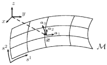
Figure 1: Geometry of a surface

Membrane kinematics.

The bilayer membrane is described as a two-dimensional surface $\mathcal{M}$ embedded in three-dimensional space (Fig.1), parameterized by curvilinear coordinates $\{s^{1},s^{2}\}$, such that its position is given by the map $\bm{x}:\mathbb{R}^{2}\to\mathbb{R}^{3}$. With standard definitions from differential geometry [27, 28] we can span the surface tangent plane with both (covariant) basis vectors $\bm{a}_{\alpha}=\frac{\partial\bm{x}}{\partial s^{\alpha}}\equiv\bm{x}_{,\alpha}$ and dual (contravariant) basis vectors $\bm{a}^{\alpha}$ defined such that $\bm{a}^{\alpha}\cdot\bm{a}_{\beta}=\delta^{\alpha}_{\beta}$. The covariant and contravariant surface metric tensors are then

$$a_{\alpha\beta}=\bm{a}_{\alpha}\cdot\bm{a}_{\beta},\quad\text{and}\quad a^{\alpha\beta}=\bm{a}^{\alpha}\cdot\bm{a}^{\beta},$$ (1)

and the determinant of the covariant metric tensor will be denoted

$$a=\det a_{\alpha\beta}.$$ (2)

The normal to the surface is

$$\bm{d}\equiv\bm{a}_{3}=\frac{\bm{a}_{1}\times\bm{a}_{2}}{|\bm{a}_{1}\times\bm{a}_{2}|}=\frac{\bm{a}_{1}\times\bm{a}_{2}}{\sqrt{a}}.$$ (3)

The curvature tensor $\mathbf{B}$ is defined by its covariant components

$$b_{\alpha\beta}=-\bm{d}_{,\alpha}\cdot\bm{a}_{\beta}=\bm{d}\cdot\bm{x}_{,\alpha\beta}=\bm{d}\cdot\bm{a}_{\alpha,\beta}.$$ (4)

The mean curvature is one half of the trace of the curvature tensor

$$H=\frac{1}{2}b^{\alpha}_{\alpha}=\frac{1}{2}a^{\alpha\beta}b_{\alpha\beta}=-\frac{1}{2}a^{\alpha\beta}(\bm{d}_{,\alpha}\cdot\bm{a}_{\beta})=-\frac{1}{2}\bm{a}^{\alpha}\cdot\bm{d}_{,\alpha}$$ (5)

(where $a^{\alpha\beta}$ is the contravariant metric tensor, defined such that $a^{\alpha\beta}a_{\alpha\beta}=\delta^{\alpha}_{\beta}$), and the Gaussian curvature is the determinant of the curvature tensor

$$K=\det\mathbf{B}=\det b_{\alpha\beta}.$$ (6)

Lipid bilayer mechanics.

We describe the energetics of the membrane by the Helfrich model [4], which assumes a strain energy of the form

$$E[\bm{x}]=\int_{\mathcal{M}}\frac{1}{2}\mathcal{K}_{C}(2H-C_{0})^{2}\sqrt{a}d^{2}s+\int_{\mathcal{M}}\mathcal{K}_{G}K\sqrt{a}d^{2}s$$ (7)

where $\mathcal{K}_{C}$ is the bending modulus and $\mathcal{K}_{G}$ is the Gaussian curvature modulus. By the Gauss-Bonnet theorem [27], the integral of Gaussian curvature is a topological constant $\int_{\mathcal{K}_{G}}K\sqrt{a}d^{2}s=4\pi(1-g)$, with $g$ being the genus, i.e. the number of handles, and thus can be neglected.

The weak form of equilibrium for the membrane can be obtained in general by the principle of virtual work, and for the case of conservative loads by minimization of total potential energy. The later dictates that the total potential energy by stationary with respect to any arbitrary admissible surface variation $\delta\bm{x}$

$$\delta\Pi\equiv\delta E-\delta W^{\text{ext}}=0.$$ (8)

Here $\delta E$ is the first variation of the membrane bending energy, and $\delta W^{\text{ext}}=\int_{\mathcal{M}}\bm{f}^{\text{ext}}\cdot\delta\bm{x}\sqrt{a}$ is virtual work done by conservative external forces $\bm{f}^{\text{ext}}$. A straightforward calculation [17] gives the first variation of the total energy as

$$\delta\Pi=\int_{\mathcal{M}}\left[\bm{n}^{\alpha}\cdot\delta\bm{a}_{\alpha}+\bm{m}^{\alpha}\cdot\delta\bm{d}_{,\alpha}-\bm{f}^{\text{ext}}\cdot\delta\bm{x}\right]\sqrt{a}{ds^{1}}{ds^{2}},$$ (9)

where we have defined stress resultants $\bm{n}^{\alpha}$ and moment resultants $\bm{m}^{\alpha}$ as

$$\bm{n}^{\alpha}=\mathcal{K}_{C}(2H-C_{0})a^{\alpha\beta}\bm{d}_{,\beta}+\mathcal{K}_{C}\frac{1}{2}(2H-C_{0})^{2}\bm{a}^{\alpha}\qquad\bm{m}^{\alpha}=-\mathcal{K}_{C}(2H-C_{0})\bm{a}^{\alpha}.$$ (10)

Enforcing constraints: augmented Lagrangian method.

Admissibility requirements on trial functions $\bm{x}$ and variations $\delta\bm{x}$ include the satisfaction of any active constraints, such as the aforementioned constraints on total surface area and enclosed volume. Here we will enforce these constraints with the augmented Lagrangian (AL) approach (see, e.g., [29]). The AL method may be thought of as a hybrid between penalty and Lagrange multiplier methods. The basic idea of AL is to solve iteratively for a Lagrange multiplier, computing multiplier updates from a penalty term. To enforce constraints on both area and volume of a membrane, we establish a sequence of modified energy funcitonals, the $n$th of these taking the the form $I^{n}=\Pi+I^{\text{con}}$, where $I^{\text{con}}$ is a constraint energy term

$$I^{\text{con}}=\frac{\mu_{V}}{2}(V-\bar{V})^{2}-p^{n}V+\frac{\mu_{A}}{2}(A-\bar{A})^{2}+\alpha^{n}A.$$

Here $\bar{A}$ and $\bar{V}$ are the specified surface area and enclosed volume of the membrane, $\mu_{A}$ and $\mu_{V}$ are penalty parameters (large and positive), and $\alpha^{n}$ and $p^{n}$ are tension and pressure multiplier estimates for the $n$th iteration. Minimization of the modified energy (holding multiplier estimates fixed) yields

$$\delta I^{n}=\delta\Pi-p^{n+1}\delta V+\alpha^{n+1}\delta A=0,$$

where $p^{n+1}=p^{n}-\mu_{V}(V_{n}-\bar{V})$ and $\alpha^{n+1}=\alpha^{n}+\mu_{A}(A_{n}-\bar{A})$ are the updated multiplier estimates. Iteration of minimization followed by multiplier updates is continued until constraints are satisfied to within some preselected tolerance, TOL, as shown below in Algorithm 1. In this way the modified energy converges to the pure Lagrange-multiplier constrained functional, with the added benefit of avoiding the associated saddle-point problem, retaining a minimization structure which is convenient for nonlinear optimization algorithms.

Whereas pure penalty methods require very large penalty parameters for accurate constraint enforcement, the AL iterative updates can achieve accuracy with much smaller penalty terms. In practice this is an important advantage, since when the penalty parameters $\mu_{V}$ and $\mu_{A}$ become large, numerical minimization becomes difficult as the Hessian $\nabla^{2}E$ (or stiffness matrix) becomes quite ill conditioned near the minimizer. This property makes minimization algorithms like quasi-Newton and conjugated gradient perform poorly, as finding the search directions becomes difficult [29]. However, small penalty parameters can produce a large number of AL iterations for convergence. Hence, it is common in practice to incrementally increase penalty parameters by some factor, FAC, after each AL iteration process to achieve faster convergence. These penalty parameter updates are also included in Algorithm 1.

Algorithm 1 Augmented Lagrangian method to enforce global area and volume constraints.

  Initialize: $p^{0}$, $\alpha^{0}$, $\mu_{V}^{0}$, $\mu_{A}^{0}$,

  Set n=0

  repeat

     Minimize $I^{n}=\Pi+\frac{\mu_{V}}{2}(V-\bar{V})^{2}-p^{n}V+\frac{\mu_{A}}{2}(A-\bar{A})^{2}+\alpha^{n}A$

     Updates:  $p^{n+1}=p^{n}-\mu_{V}^{n}(V_{n}-\bar{V})$ ,  $\alpha^{n+1}=\alpha^{n}+\mu_{A}^{n}(A_{n}-\bar{A})$  $\mu_{V}^{n+1}=\mu_{V}^{n}\times\text{FAC}$ ,  $\mu_{A}^{n+1}=\mu_{A}^{n}\times\text{FAC}$  $n\leftarrow n+1$

  until  $|V^{n}-\bar{V}|<\text{TOL}\quad\text{and}\quad|A^{n}-\bar{A}|<\text{TOL}$

Finite element approximation.

A FE approximation is introduced by replacing the field $\bm{x}$ with the approximated field $\bm{x}_{h}$ defined by

$$\bm{x}_{h}(s^{1},s^{2})=\sum_{a=1}^{N}\bm{x}_{a}N^{a}(s^{1},s^{2})$$ (11)

where the $N^{a}(s^{1},s^{2}),~{}a=1,\dots,N$ are shape functions of the FE mesh, and their coefficients, $\bm{x}_{a}$ are the positions of the nodal control vertices. Introducing this approximation into the modified energy funcitonal upon minimization leads to a set of discrete approximate equilibrium equations

$$\bm{f}^{\text{int}}_{a}+\bm{f}^{\text{con}}_{a}-\bm{f}^{\text{ext}}_{a}=0.$$ (12)

Here $\bm{f}^{\text{int}}_{a}$ are the internal nodal forces due to bending of the membrane,

$$\bm{f}^{\text{int}}_{a}=\int_{\mathcal{M}}\left[\bm{n}^{\alpha}\cdot\frac{\partial\bm{a}_{\alpha}}{\partial\bm{x}_{a}}+\bm{m}^{\alpha}\cdot\left(\frac{\partial\bm{d}}{\partial\bm{x}_{a}}\right)_{,\alpha}\right]\sqrt{a}{d^{2}s};$$ (13)

$\bm{f}^{\text{con}}_{a}$ are the constraint nodal forces due to the pressure and tension that are conjugate to the constrained volume and area,

$$\bm{f}^{\text{con}}_{a}=-p^{n+1}\frac{\partial V}{\partial\bm{x}_{a}}+\alpha^{n+1}\frac{\partial A}{\partial\bm{x}_{a}};$$ (14)

and $\bm{f}^{\text{ext}}_{a}$ are the external nodal forces, due to the application of distributed loads on the surface,

$$\bm{f}^{\text{ext}}_{a}=\int_{\mathcal{M}}\bm{f}^{\text{ext}}N^{a}\sqrt{a}{d^{2}s}.$$ (15)

Note that the integrands of the global expressions for internal and constraint forces are described in more explicit detail in [17]. Following that work, we again employ $C^{1}$-conforming subdivision surface shape functions [30, 31] along with second-order (three-point) Gaussian quadrature for the computation of element integrals.

2.2 Viscous regularization of tangential mesh deformation

In the curvature model, the energy is determined by the mean curvature which is a parameterization-independent property of the surface shape, and thus is not sensitive to in-plane dilatational or shearing deformations of the surface FE mesh. Much like physical lipid molecules, FE nodes can flow freely on the deformed surface. As discussed in [17], this fact is manifested in the appearance of degenerate, zero-stiffness, zero-energy modes. Here we discuss the implementation of an artificial viscosity method designed to numerically eliminate these degenerate modes.

For solid shells having both reference and deformed configurations, in-plane deformations (dilatation and shearing) can thus be expressed locally in terms of first derivatives of the surface position maps of these two configurations. In curvature model,a well-defined reference configuration does not exist since the energy is only related to the deformed shape. The basic ingredients for stabilization of these tangential modes are the introduction of a reference configuration and an energy term elastically penalizing in-plane deformation away from this reference state. However, to retain the physics of the original model, the addition of any in-plane elastic energy must result in a variational problem possessing the same minimizing solution as the original problem. In other words, the artificial in-plane energy must attain a value of zero when the entire model is in equilibrium. To design an algorithm that achieves these goals, we define a sequence of variational problems, minimizing a modified energy functional

$$I^{n}=\Pi[\bm{x}]+I^{\text{con}}[\bm{x}]+I^{\text{reg}}[\bm{x};\bm{X}^{n}]$$ (16)

where the reference configuration $\bm{X}^{n}$ for the $n$th iteration is the deformed solution $\bm{x}^{n-1}$ of the previous iteration. The form of the regularization energy $I^{\text{reg}}[\bm{x};\bm{X}]$ can be chosen such that it vanishes when $\bm{x}=\bm{X}$, to ensure that solutions $\bm{x}^{n}$ converge to minimizers of the original unregularized problem with increasing $n$. This regularization method is outlined below in Algorithm 2.

Algorithm 2 Viscous regularization via reference updates.

  Set $X^{0}=$ initial shape.

  Set $n=0$

  repeat

     Minimize $I^{n}=\Pi[\bm{x}]+I^{\text{con}}[\bm{x}]+I^{\text{reg}}[\bm{x};\bm{X}^{n}]\quad\rightarrow\quad\text{solution, }\bm{x}^{n}$

     Update reference: set $\bm{X}^{n+1}=\bm{x}^{n}$

     $n\leftarrow n+1$

  until $I^{\text{reg}}[\bm{x}^{n};\bm{X}^{n}]<\text{TOL}$

Qualitatively, assignment of the reference configuration for each iteration to be the current configuration of the previous iteration results in a type of algorithmic viscosity, producing forces that resist the motion of nodes away from their position at each previous iteration. The quantitative details of this viscosity depend on the particular form chosen for the in-plane regularization energy, $I^{\text{reg}}$. Here we give two example forms, the first derived from planar continuum elasticity theory and the second representing the mesh as a network of viscous dashpot elements.

Continuum elastic regularization energy.

Here we treat the in-plane deformation response for each regularization iteration as that of a two-dimensional solid membrane. This local response can be modeled via a hyperelastic strain energy density, $w(\mathbf{F})$, which is a function of the surface deformation gradient

$$\mathbf{F}=\bm{a}_{\alpha}\otimes\bm{A}^{\alpha},$$ (17)

where $\bm{A}^{\alpha}$ are the dual basis vectors on the reference surface, i.e., $\bm{A}^{\alpha}\cdot\bm{A}_{\beta}=\delta^{\alpha}_{\beta}$, where $\bm{A}_{\alpha}=\bm{X}^{n}_{,\alpha}$. Thus the regularization energy becomes

$$I^{\text{reg}}[\bm{x};\bm{X}^{n}]=\int_{\mathcal{M}}w(\mathbf{F})\sqrt{A}d^{2}s.$$ (18)

To preserve objectivity, the strain energy is a function of $\mathbf{F}$ through implicit dependence on the invariants of the surface-Right-Cauchy-Green deformation tensor $\mathbf{C}=\mathbf{F}^{\textsf{T}}\cdot\mathbf{F}=a_{\alpha\beta}\bm{A}^{\alpha}\otimes\bm{A}^{\beta}$ [32]. As $\mathbf{C}$ is a rank-2 tensor, the two non-zero principal invariants are

$$I_{1} =\text{tr}(\mathbf{C})=\bar{a}^{\alpha\beta}a_{\alpha\beta}$$ (19a)

$$I_{2} =\frac{1}{2}\{[\text{tr}(\mathbf{C})]^{2}-\text{tr}(\mathbf{C}^{2})\}=\frac{1}{2}\{(\bar{a}^{\alpha\beta}a_{\alpha\beta})^{2}-\bar{a}^{\alpha\mu}\bar{a}^{\beta\nu}a_{\alpha\beta}a_{\mu\nu}\}\equiv J^{2}.$$ (19b)

The strain energy density is thus a function of these two invariants

$$w(\mathbf{F})=w(I_{1},I_{2}).$$

As a specific example, consider a strain energy function that decouples the dilatational, and shear responses, as used by Evans and Skalak [33] to model the red blood cell cytoskeleton

$$w=\underbrace{\frac{k}{2}(J-1)^{2}}_{\text{area change}}+\underbrace{\mu\left(\frac{\text{tr}(\mathbf{C})}{2J}-1\right)}_{\text{shear}}.$$

Here $k$ and $\mu$ are stretching and shear moduli, respectively. It should be carefully noted that although we follow here the formalism of solid mechanics, the reference configuration $\bm{X}^{n}$ is not permanent as for a solid; rather the reference configuration is iteratively updated so that the resulting stresses may relax to zero.

Dashpot regularization energy.

The viscous character of our proposed scheme is much more obvious when we compose the regularization energy of contributions from Hookean springs placed along all element edges, namely,

$$I^{\text{reg}}=\sum_{\text{edge }ab}\frac{k}{2}(\ell_{ab}-L_{ab})^{2},$$ (20)

where $\ell_{ab}=|\bm{x}_{a}-\bm{x}_{b}|$ and $L_{ab}=|\bm{X}_{a}^{n}-\bm{X}_{b}^{n}|$ are the lengths of the edge connecting mesh vertices $a$ and $b$ in the deformed and current configurations, respectively. Differentiating this energy, the corresponding force on a node $a$ from the spring connecting it along an edge to node $b$ can be obtained as

$$\bm{f}_{ab}=k(\ell_{ab}-L_{ab})\bm{n}_{ab}$$

where $\bm{n}_{ab}$ is the unit vector pointing from node $a$ to node $b$. Recalling that the reference configuration for the $n$th iteration is the same as the deformed configuration of the $n-1$th iteration, the magnitude of this force can also be written as

$$f_{ab}=k(\ell_{ab}^{n}-\ell_{ab}^{n-1}).$$

This is easily identified as the backward-Euler time-discretization of the force-velocity relation for a viscous dashpot

$$f_{ab}=k\frac{\partial\ell_{ab}}{\partial t},$$

Thus, iterative reference updates of the form $\bm{X}^{n}=\bm{x}^{n-1}$ have the effect of converting a network of springs into a network of dashpots, clearly revealing the viscous character of the regularization scheme.

We have numerically implemented both the continuum elastic and dashpot regularization described here, and although both forms are effective in practice we have preferred the dashpot approach for its simplicity, efficiency, and robustness. The remainder of the paper focuses on the use of this second approach, demonstrating its effectiveness in application.

3 Applications

3.1 Shape vs. reduced volume

Even in the absence of any externally applied loads, the two constraints on area and volume cause vesicles to transition among a variety of interesting equilibrium shapes. Here some of the calculations performed in [17] of the equilibrium shapes for different reduced volumes are repeated, as a first demonstration of the effectiveness of viscous regularization.

Reduced volume $\nu$ is a geometrical quantity defined as

$$\nu=\frac{V}{(4\pi/3)R{{}_{0}}^{3}},$$ (21)

where $R_{0}=\sqrt{A/4\pi}$ is the radius of a sphere with the area $A$ of the vesicle. Reduced volume is then written as

$$\nu=\frac{6\sqrt{\pi}V}{A^{3/2}}.$$ (22)

The reduced volume is the ratio of the current volume of the vesicle and the maximum volume that the current total area of vesicle can ensphere. For a spherical vesicle, the reduced volume $\nu=1$; a vesicle of any other shape has $0<\nu<1$.

To compute the following results, the spontaneous curvature model is used with $C_{0}=0$. The modified energy is computed with loop subdivision shell elements and second-order (three-point) Gaussian quadrature, and minimized with the quasi-newton L-BFGS-B solver [34, 35, 36].

Viscous regularization.

As a first assessment of the benefit of regularization, results are compared with the simulations done in [17], in which local area and global volume constraints were performed by penalty method instead of AL method. First, the same calculation of [17] is repeated; then the viscous regularization is added, with same kind of constraints (local area and global volume constraint) and penalty parameters ($\mu_{A}=10^{4}R^{2}/\mathcal{K}_{C}$ for local area constraint and $\mu_{A}=5\times 10^{4}R^{2}/\mathcal{K}_{C}$ for global volume constraint).

The calculation starts from an initial ellipsoid shape which has a reduced volume $\nu=0.914$ (Fig. 2). In the calculation, the area is fixed at its initial value and the volume is reduced in order to satisfy the constraint on $\nu$. For each simulation, violation of the volume constraint subjects the vesicle to a large pressure according to the penalty term in the functional. The energy is then relaxed by L-BFGS-B minimization and result in the equilibrium shapes. The iteration of of reference updates in Algorithm 2 is continued until the regularization energy is sufficiently small, $I^{\text{reg}}/I<10^{-5}$. In all the simulations, the same mesh, made up of 642 vertex nodes and 1280 elements, is used.

The resulting equilibrium shapes for $\nu=0.9$ and $\nu=0.8$ are shown in Fig. 2. Starting from the initial shape, the equilibrium shape for $\nu=0.9$ is computed by minimizing the energy; then from the resulting $\nu=0.9$ shape, setting $\nu=0.8$, the equilibrium shape for $\nu=0.8$ is computed. The computational cost with and without the viscous regularization is listed in Table 1. As can be seen, the convergence rate is highly improved (almost two orders of magnitude faster) with the viscous regularization while the resulting shapes are equivalent. For different choices of spring constant $k$, the computational cost also varies. The computational cost has two contributions: one is the iteration number for each minimization; the other is the number of reference updates required to satisfy the convergence criterion $I^{\text{reg}}/I<10^{-5}$. These both depend on $k$. For each minimization, the larger $k$ is, the smaller the iteration number will be. While for the number of reference updates, it is opposite: the larger $k$ is, the more reference updates needed. For example, to get the equilibrium shape $\nu=0.9$ from the initial shape, $kR^{2}/\mathcal{K}_{C}$=1 requires 2 reference updates, each of which costs $\approx 1000$ iterations for minimization; while for $kR^{2}/\mathcal{K}_{C}$=100, there are 20 reference updates each costing $\approx 250$ minimization iterations. In this case $kR^{2}/\mathcal{K}_{C}$=1 works the best, but the optimal $k$ depends on the specific problem. In the later sections on tether formation, a much larger $k$ ($kR^{2}/\mathcal{K}_{C}$=1000) is used.

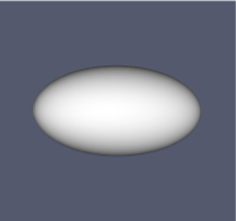
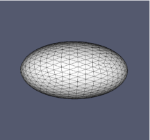
(a) Initial shape, $\nu=0.914$ (not in equilibrium)

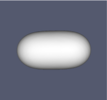
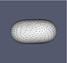
(b) $\nu=0.9$ without regularization.

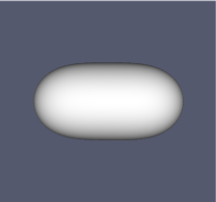
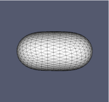
(c) $\nu=0.9$ with regularization.

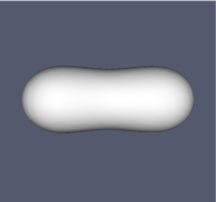
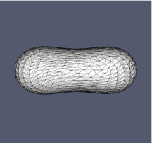
(d) $\nu=0.8$ without regularization.

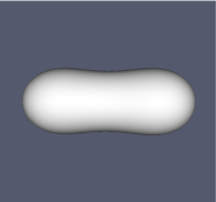
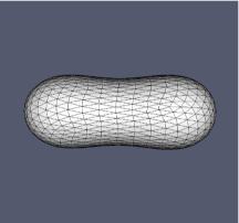
(e) $\nu=0.9$ with regularization.

Figure 2: Limit surfaces and control meshes of equilibrium shapes for $\nu=0.9$ and $\nu=0.8$.

Computational cost with and without the viscous regularization
$kR^{2}/\mathcal{K}_{C}$	Total iterations (initial shape $\rightarrow\nu=0.9$)	Total iterations ($\nu=0.9\rightarrow 0.8$)
0	35,950	603,858
0.5	2,304	287,825
1	1,821	9,482
10	2,122	12,480
100	4,776	79,038

Table 1: Viscous regularization improves the convergence rate of L-BFGS-B minimization. The first row $kR^{2}/\mathcal{K}_{C}=0$, shows the results without the viscous regularization, which are identical to the approach used in [17]. ($k$: spring constant; $R$: average radius of the vesicle; $\mathcal{K}_{C}$: bending modulus.)

Augmented Lagrangian constraint enforcement.

From the results described above, viscous regularization is shown to be able to heavily lower the computational cost when a penalty method is used to enforce the constraints on area and volume. However, regularization also eliminates the need for local enforcement of incompressibility. Global constraints on area and volume can be easily implemented via the augmented Lagrangian (AL) method which is more efficient than the previous penalty method. Here, the shape change from the initial ellipsoid shape to the equilibrium shape of $\nu=0.9$ is used to compare the penalty method with the AL method. In this test global area and global volume constraints are carried out first by the penalty method with a range of penalty parameters, and secondly with the AL method. Viscous regularization is used for both the penalty method and the AL method. Iteration of reference updates is continued until the regularization energy is sufficiently small, $I^{\text{reg}}/I<2.0\times 10^{-5}$.

The regularization spring constant $k$ is set to be $k=10\mathcal{K}_{C}/R^{2}$, where $R$ is the average radius of the vesicle and $\mathcal{K}_{C}$ is the bending modulus. For the AL method, the penalty parameters are initialized to be a fairly small number ($\mu_{V}=10^{4},\mu_{A}=10^{4}$), and are then increased by a factor of 2 for each of the following minimizations. The minimization continues until the constraints on area and volume are satisfied to within a tolerance and the regularization energy is sufficiently small. Viscous regularization reference updates are included with AL multiplier updates in a single iteration loop. This hybrid regularization-AL algorithm, shown in Algorithm 3, is a combination of separate Algorithms 1 and 2.

Algorithm 3 Hybrid algorithm combining AL constraint enforcement with viscous regularization.

  Initialize: $p^{0}$, $\alpha^{0}$, $\mu_{V}^{0}$, $\mu_{A}^{0}$, $X^{0}=$ initial shape, $\bar{\nu}=0.9$ (the specified reduced volume).

  Set $n=0$

  repeat

     Minimize $I^{n}=\Pi[\bm{x}]+\frac{\mu_{V}}{2}(V-\bar{V})^{2}-p^{n}V+\frac{\mu_{A}}{2}(A-\bar{A})^{2}+\alpha^{n}A+I^{\text{reg}}[\bm{x};\bm{X}^{n}]$

     $\rightarrow\quad\text{solution, }\bm{x}^{n}$

     Update reference: set $\bm{X}^{n+1}=\bm{x}^{n}$

     if $|\nu_{n}-\bar{\nu}|/\bar{\nu}>\text{TOL}_{1}$ then

        AL Updates:  $p^{n+1}=p^{n}-\mu_{V}^{n}(V_{n}-\bar{V})$ ,  $\alpha^{n+1}=\alpha^{n}+\mu_{A}^{n}(A_{n}-\bar{A})$  $\mu_{V}^{n+1}=\mu_{V}^{n}\times\text{FAC}$ ,  $\mu_{A}^{n+1}=\mu_{A}^{n}\times\text{FAC}$

     end if$n\leftarrow n+1$

  until $|\nu_{n}-\bar{\nu}|/\bar{\nu}<\text{TOL}_{1}$ and $I^{\text{reg}}[\bm{x}^{n};\bm{X}^{n}]<\text{TOL}_{2}$

As the Table 2 shows, the AL method reduces the computational cost significantly. This is especially true when high accuracy of the constraints is desired, in which case the penalty method requires extremely large parameters, which lead to conditioning problems that impede convergence of the nonlinear solver. Indeed, for penalty parameter $>10^{8}$, L-BFGS-B iterations diverge. In contrast, for the AL method to achieve high accuracy penalty parameters need not be very large [29].

Penalty method vs. AL method
Accuracy $|\nu-0.9|/0.9$	$10^{-2}$	$10^{-3}$	$10^{-4}$	$10^{-5}$	$10^{-6}$	$10^{-7}$	$10^{-8}$	$10^{-9}$	$10^{-10}$
Penalty parameter	$10^{4}$	$10^{5}$	$10^{6}$	$10^{7}$	$10^{8}$	n/a	n/a	n/a	n/a
Iterations (penalty method)	379	436	1032	3455	9231	n/a	n/a	n/a	n/a
Iterations (AL method)	366	425	500	515	616	743	916	981	1201

Table 2: Computational cost of the penalty method and the AL method. To achieve the same accuracy, the AL method requires fewer total iterations compared to the penalty method. More importantly, for extremely high accuracy ($<10^{-7}$), the L-BFGS-B minimization diverges with the penalty method, while the AL method still converges.

3.2 Tether formation

A point-force acting on lipid membranes can pull out a long narrow tube commonly called a tether. This can be done by using micropipettes [e.g., 23], optical tweezers [e.g., 37], or even growing microtubules inside the vesicle [37]. The mechanical reason for formation of tethers lies in the lack of shearing modulus for membranes. Elongating in one direction and contracting in the other to such a spectacular way like tethers mechanically means extremely large shear deformations [38, 39, 40, 41].

Since tether simulation involves very large deformations, the triangles in the finite element mesh are subject to severe distortions. In practice, as elements become more distorted, the zero-energy tangential modes can actually become numerically unstable (Fig. 3). Viscous regularization has to be added in order to suppress these zero-energy modes. Furthermore, the critical force to pull out a tether is very sensitive to pressure and surface tension. Numerically, this necessitates highly accurate enforcement of the volume and area constraints. For a penalty method this implies very large penalty parameters, which lead to conditioning problems (e.g., Table 2). For this reason, here the augmented Lagrangian method is applied.

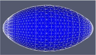
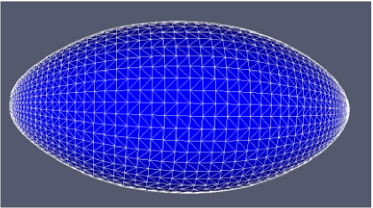
Figure 3: The equilibrium shape of a vesicle of reduced volume $\nu=0.9$ with external forces ($\approx$ 1 pN) applied at the two ends (forces not shown), mesh without (left figure) and with (right figure) the viscous regularization. Note that the unstabilized mesh is subject to element distortion even at small applied load.

Starting from an initial equilibrium shape (prolate), tether development is simulated by incrementally displacing nodes at the tips of the vesicle, and performing energy minimization resulting in the equilibrium tethered shapes for each extension. However, even with the viscous regularization, the mesh can still be distorted by the dramatic deformations experienced at larger extensions. Therefore, re-meshing is performed at intervals of the extension. Fig. 4 shows snapshots from a typical simulation for reduced volume $\nu=0.9$.

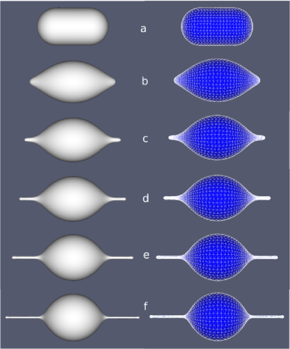
Figure 4: The tethering of a vesicle starting from a prolate of reduced volume $\nu=0.9$. Left: limit surfaces of equilibrium shapes; right: control meshes. Number of nodes and elements: (a) 4202 nodes, 8400 elements; (b) & (c) 4682 nodes, 9360 elements; (d) 6202 nodes, 12400 elements; (e) & (f) 8682 nodes, 17360 elements. End to end distance: (a) 6.8$\mu$m, (b) 8.2$\mu$m, (c) 9.2$\mu$m, (d) 10.2$\mu$m, (e) 11.6$\mu$m, and (f) 12.8$\mu$m

Applied forces.

The reaction forces conjugate to specified end displacements can also be calculated by simply adding up all internal forces of the fixed nodes (Eq. 13). The force vs. end-to-end distance results for the vesicles in Fig. 4 are shown in Table 3, with $r$ the radius of the tethers ($\mu$m) and bending modulus $\mathcal{K}_{C}=15K_{b}T$ [37]. Although an exact analytical solution for the force-extension relation is not possible, a simple analytical estimate [39] is used to compare with the computed results from the simulation. The estimate assumes that the thin tube (tether) is pulled out from a sphere, and the sphere remain unchanged during the pulling (Fig. 5). The analytical estimated force and surface tension are given as [39]:

$$F=2\pi\mathcal{K}_{C}/r,$$ (23)

and the surface tension

$$\alpha=0.5\mathcal{K}_{C}/r^{2},$$ (24)

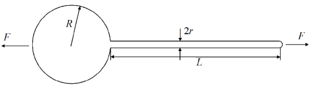
Figure 5: Schematic of the tethered shape

Force vs. end-to-end distance
End-to-end distance ($\mu$m)	6.8	8.2	9.2	10.2	11.6	12.8
Computed tether radius ($\mu$m)	n/a	n/a	0.20	0.165	0.140	0.105
Computed force (pN)	0	1.41	1.76	2.14	2.72	3.68
Analytical estimated force (pN)	n/a	n/a	1.88	2.29	2.69	3.59
Computed tension (pN/$\mu$m)	0.05	0.43	0.71	0.98	1.60	2.93
Analytical estimated tension (pN/$\mu$m)	n/a	n/a	0.75	1.10	1.53	2.72

Table 3: Computed and analytical estimated forces for each tethered shape. For the shape in Fig. 4(c), the computed tether radius is not uniform along the extension direction, and $r=0.20\mu$m is an estimate. As noted in the text a bending modulus of $\mathcal{K}_{C}=15K_{b}T$ is used for all calculations.

As Table 3 shows, for well developed tethered shapes (end-to-end distance 11.6 and 12.8 $\mu$m, vesicle (e) and (f) in Fig. 4), the computed results and analytical estimations are very close. It is a notable advantage that the present simulation framework is also capable of force-extension calculations for shapes that are not as simple as the schematic in Fig.5. Although the present example is in fact axisymmetric, the algorithms are fully three-dimensional and can be applied to loadings and shapes lacking symmetry.

3.3 Lipid Phase Separation

Membranes formed from different lipids can separate into distinct domains (phases) according to their chemical properties, leading to the formation of buds [42, 43]. Baumgart et al. [44] found that their experiments are in good agreement with line tension theory [45, 46, 47], which treats domain interfaces as discrete with an interface energy proportional to their length. An alternative, smooth-interface approach, based on traditional Ginzburg-Landau (GL) theory [48, 49] can be used to also model phase separation [50, 51, 52, 53, 54]. One major drawback of the line tension model is that it requires the system to be pre-phase-separated into well-defined domains, preventing the consideration of composition dynamics.

Here a GL model for a multi-component bilayer with two different lipids in equilibrium is formulated, assuming that the vesicle is composed of a mixture of two lipids denoted $A$ and $B$. In general, these two lipid types may have different constitutive properties, as modeled by separate constitutive parameters: $\{\mathcal{K}_{C}^{(A)},\mathcal{K}_{G}^{(A)},C_{0}^{(A)}\}$ for lipid $A$, and $\{\mathcal{K}_{C}^{(B)},\mathcal{K}_{G}^{(B)},C_{0}^{(B)}\}$ for lipid $B$.

Let the local concentrations of the two lipids be described by the concentration parameters $c^{(A)},c^{(B)}\in[0,1]$ with $c^{(A)}+c^{(B)}=1$. The local lipid concentration at point $\mathsf{s}=(s^{1},s^{2})$ can then be described by an order-parameter field $c(\mathsf{s})\equiv c^{(A)}$, which is referred to as the concentration field or phase field. The local constitutive properties of the membrane can then be modeled as functions of the phase field with convex combinations of the pure phase parameters:

$$\mathcal{K}_{C} =c\mathcal{K}_{C}^{(A)}+(1-c)\mathcal{K}_{C}^{(B)}$$ (25a)

$$\mathcal{K}_{G} =c\mathcal{K}_{G}^{(A)}+(1-c)\mathcal{K}_{G}^{(B)}$$ (25b)

$$C_{0} =cC_{0}^{(A)}+(1-c)C_{0}^{(B)}$$ (25c)

Thus rewriting the strain energy including explicit dependence of fields on surface position,

$$E=\int_{\mathcal{M}}\left\{\frac{1}{2}\mathcal{K}_{C}(\mathsf{s})[2H(\mathsf{s})-C_{0}(\mathsf{s})]^{2}+\mathcal{K}_{G}(\mathsf{s})K(\mathsf{s})\right\}\sqrt{a}{d^{2}s}$$ (26)

where explicit dependence of the mechanical properties on surface coordinates $\mathsf{s}$ has been noted as a reminder of the heterogeneity of the system.

The mechanics of the membrane are then dependent on both the shape of the vesicle and the lipid composition. Minimization of the total potential energy now yields two sets of Euler-Lagrange equations, one being the equilibrium equations related to variations in the shape $\delta\bm{x}$, and the other being a phase equilibrium equation related to variations in the concentration $\delta c$.

One further modification to the energy functional is needed to build into the model of the physics of phases separation [49].

$$I=E+\int_{\mathcal{M}}\Delta E[\psi({c})+\epsilon^{2}|\nabla{c}|^{2}]\sqrt{a}d^{2}s.$$ (27)

Here the normalized GL energy $\psi({c})$ is a double-well potential such as

$$\psi({c})=16c^{2}(c-1)^{2}$$

(see Fig. 6) which is minimized when the concentration $c$ takes a value of either 0 or 1, corresponding to local lipid concentration of either pure type $A$ or pure type $B$. The parameter $\Delta E$ scales the height of the barrier between the two minima of $\psi({c})$, and controls the energy cost of a domain interface. The second addition to the energy describes short-range cooperativity between neighboring lipids. The parameter $\epsilon$ is essentially a length scale which will determine the width of the region of transition between phases. As $\epsilon$ decreases to zero, this region will limit to a curve where the concentration gradient can be non-zero. Inclusion of this penalty term in the energy will then produce the effect of a diffuse line tension in the transition between regions of pure phases.

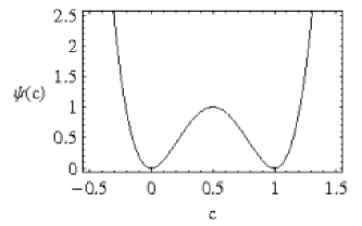
Figure 6: Double-well normalized GL energy $\psi({c})=16c^{2}(c-1)^{2}$ used to model phase segregation in a two-component lipid system.

In Baumgart’s experiment [42, 44], bending modulus $\mathcal{K}_{C}\approx 10^{-19}J$, line tension $\sigma\approx 10^{-12}N$, and the radius of the vesicle $R\approx 10\mu m$. Two vesicles from [44] are simulated: one with reduced volume $\nu=0.98$, phase $B$ area fraction $x_{B}=(1/A)\int cdA=0.89$; the other $\nu=0.76$, $x_{B}=(1/A)\int cdA=0.56$, starting from the original spherical shape with two separate domains (Fig. 2A and 2G in [44]). For the first one ($\nu=0.98$), the simulation captured the small cap seen in the experiment (Fig. 7).

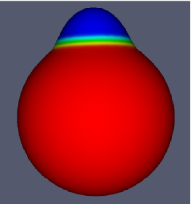
(a) Simulation

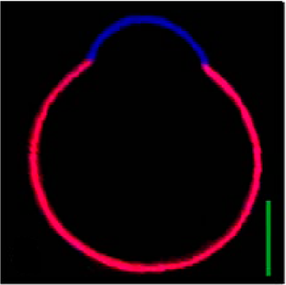
(b) Experiment (Fig. 2G from [44])

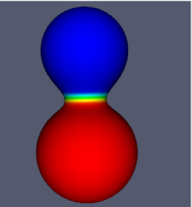
(c) Simulation

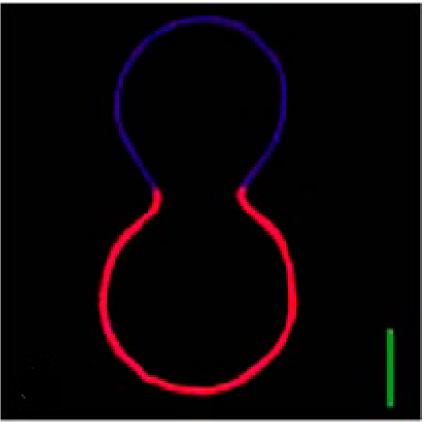
(d) Experiment (Fig. 2A from [44])

Figure 7: Comparison of simulation and experiment for two component lipid phase separation. (a) & (b) have reduced volume $\nu=0.98$ and global concentration $x_{B}=0.98$. (c) & (d) have $\nu=0.76$ and $x_{B}=0.56$. Phase $A$ ($c=0$) is colored blue; phase $B$ ($c=1$) is colored red. Scale bars are $5\mu$m. Experimental images are taken from the work of Baumgart et al. [44].

But for $\nu=0.76$, the mesh around the interface is distorted (Fig. 8 (a)). Because the simulation starts from a sphere with roughly equilateral triangle elements, the shape change of vesicle causes the elements in the interface region to contract severely in the circumferential direction. This Element distortion needs to be suppressed because it can lead to inaccuracy and instability of the finite element simulation.

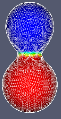
(a) standard dashpot regularization

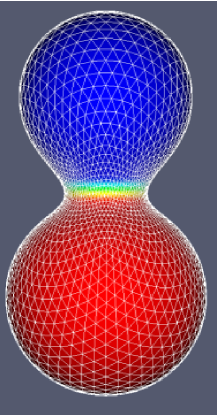
(b) r-adaptive regularization

Figure 8: r-adaptive regularization helps elements perform well in the interface ($\nu=0.76$).

In order to get a good mesh after the deformation, the elements near the interface need to contract in all directions so that they remain equilateral, resulting in a greater density of elements than other parts of the vesicle. To tackle such large deformations, remeshing strategies are often needed. The viscous regularization introduced in section 2.2 makes an r-adaptive remeshing possible, since reference configuration can be arbitrarily formulated to reposition the nodes of the mesh. Here, a slight modification of the dashpot regularization method is proposed with a reference updating strategy that drives elements toward equilateral shape.

Given an element of the mesh at regularization iteration $n-1$ with area $A_{n-1}$, r-adaptive regularization at step $n$ is defined by placing springs on the three edges all of the same reference length

$$\bar{\ell}_{n-1}=2\sqrt{\frac{A_{n-1}}{\sqrt{3}}},$$

i.e., the length of a side of an equilateral triangle of the same area $A_{n-1}$. Thus the regularization energy term for each triangle is written as

$$E_{n}=\frac{k}{2}\sum_{i=1}^{3}(\ell_{n}^{i}-\bar{\ell}_{n-1})^{2},$$ (28)

where the $\ell^{i}$ are the lengths of the element edges.

In principle this regularization energy could be applied to every element in a mesh. However, in practice these iterative updates are slow to converge to a fully relaxed state (with zero regularization energy), and depending on the regularization constant $k$ the method can get stuck in a state with finite energy stored in the springs. Hence, this “equilateral” form of the dashpot regularization is only applied selectively to poorly shape elements, all the other elements with the standard viscous regularization. A shape-criteria $\gamma$ is then formulated to calculate different spring energy for different elements,

$$\gamma=\sum_{i=1}^{3}\frac{(\ell^{i}-\bar{\ell})^{2}}{\bar{\ell}^{2}}.$$

Using this measure of shape quality, the regularization energy is defined for each triangle by

$$E_{n}=\begin{cases}\frac{k}{2}\sum_{i=1}^{3}(\ell_{n}^{i}-\bar{\ell}_{n-1})^{2},\quad\gamma\text{ large},\\ \frac{k}{2}\sum_{i=1}^{3}(\ell_{n}^{i}-\ell_{n-1}^{i})^{2},\quad\gamma\text{ small}.\end{cases}$$

In other words, if $\gamma$ is large (say, $\gamma>1$) for an element, it has poor shape and r-adaptive regularization is used on that element; if $\gamma$ is small enough, reference lengths are updated from the deformed lengths of the previous iteration as for the dashpot model described earlier. The addition of r-adaptive regularization has the effect of moving the nodes around on the membrane surface. In the present example of a phase-separated vesicle, this results in a finer mesh near the interface area than elsewhere (Fig. 8 (b)). For reduced volume $\nu=0.76$, the simulated result is shown in Fig. 7 to compare with the experimental result.

4 Conclusions

In this paper a framework for three-dimensional analysis of mechanics of lipid bilayer membranes is presented, based on the finite element method. Particular interest is focused on large deformation problems: tether formation (Sec. 3.2) and phase separation (Sec. 3.3).

The primary difficulty faced in FE simulation of fluid membranes is the presense of mesh instabilities linked to the parameterization-independent nature of fluid surfaces. Curvature models of vesicle mechanics depend only on current shape, and thus is not sensitive to in-plane (stretching and shearing) deformations of the surface FE mesh. Here a viscous regularization method is thus introduced to regularize tangential mesh deformations. In this method artificial reference configurations and corresponding in-plane energies are added to stabilize the tangential deformations; reference updates are designed so that artificial energy converges to zero in order to retain the physics of the original model.

Regulariztion of tangential mesh deformations eliminates the need for local enforcement of membrane incompressibility [17], providing a more convenient setting for augmented Lagrangian (AL) enforcement of global constraints on area and volume. The AL method can achieve higher accuracy with lower computational cost, compared to the penalty method.

Large deformation problems can be very sensitive to mesh quality. Because of the physical meaninglessness of the reference configurations in the simulation, r-adaptive remeshing is easy to achieve in the context of viscous regularization, simply choosing a reference updating strategy which will reposition the nodes to get a better quality mesh.

One promising direction for future work is to combine viscous regularization and r-adaptive remeshing with the dynamic triangulation approach [18], in which the edge of a pair of triangles swaps to form less distorted triangle elements instantly. This could be a powerful approach, speeding up the otherwise slow movements of nodes driven by the viscous regularization. Also, the success of r-adaptive regularization relies to some degree on the quality of the starting mesh. If there are too many badly shaped element and the shape criteria $\gamma$ tolerance is chosen to be too small, the mesh can sometimes lock with non-zero regularization energy, resulting in physically wrong shapes of vesicles. Dynamic triangulation could aleviate such locking. Lastly a r-adaptive regularized dynamic triangulation strategy could avoid the need for global remeshing in large deformation problems such as the tether simulations in Sec. 3.2.

Although the problems simulated in this paper are all axisymmetric, the model is really designed for fully three-dimensional calculations, and can thus deal with arbitrary geometries and loads. For example future applications such as mechanics of organelles like mitochondria [55] and endoplasmic reticulum (ER) [56], with incredibly complex shapes may provide exciting opportunities for future study with these methods.

References

- Alberts et al. [1998] B. Alberts, D. Bray, A. Johnson, J. Lewis, M. Raff, K. Roberts, and P. Walter. Essential Cell Biology. Garland Publishing, Inc, New York, 1998.
- Seifert [1997] U. Seifert. Configurations of fluid membranes and vesicles. Adv. Phys., 46(1):13–137, 1997.
- Canham [1970] P.B. Canham. The minimum energy of bending as a possible explanation of the biconcave shape of the red blood cell. Journal of Theoretical Biology, 26:61–81, 1970.
- Helfrich [1973] W. Helfrich. Elastic properties of lipid bilayers: Theory and possible experiments. Z. Naturforsch., 28c:693–703, 1973.
- Evans [1974] E.A. Evans. Bending resistance and chemically-induced moments in membrane bilayers. Biophysical Journal, 14(12):923–931, 1974.
- Svetina et al. [1982] S. Svetina, A. Ottova-Leitmanova, and R. Glaser. Membrane bending energy in relation to bilayer couples concept of red blood cell shape transformations. J. Theoret. Biol., 94:13–23, 1982.
- Svetina and Zeks [1983] S. Svetina and B. Zeks. Bilayer couple hypothesis of red cell shape transformations and osmotic hemolysis. Biochem. Biophys. Acta, 42:86–90, 1983.
- Seifert et al. [1992] U. Seifert, L. Miao, H.G. Döbereiner, and M. Wortis. The structure and conformation of amphiphilic membranes. Springer Proceedings in Physics, 66:93–96, 1992.
- Wiese et al. [1992] W. Wiese, W. Harbich, and W. Helfrich. Budding of lipid bilayer vesicles and flat membranes. J. Phys.: Condens. Matter, 4:1647–1657, 1992.
- Bozic et al. [1992] B. Bozic, S. Svetina, B. Zeks, and R.E. Waugh. Role of lamellar membrane structure in tether formation from bilayer vesicles. Biophys. J., 61:963–973, 1992.
- Jenkins [1977a] J.T. Jenkins. Static equilibrium configurations of a model red blood cell. Journal of Mathematical Biology, 4:149–169, 1977a.
- Jenkins [1977b] J.T. Jenkins. The equations of mechanical equilibrium of a model membrane. SIAM Journal on Applied Mathematics, 32(4):755–764, 1977b.
- Hsu et al. [1992] L. Hsu, Kusner R., and J. Sullivan. Minimizing the squared mean curvature integral for surfaces in space forms. Exp. Math., 1(3):191–207, 1992.
- Jaric et al. [1995] M. Jaric, U. Seifert, W. Wintz, and M. Wortis. Vesicular instabilities: the prolate-to-oblate transition and other shape instabilities of fluid bilayer membranes. Phys. Rev. Lett., 52:6623, 1995.
- Kraus et al. [1995] M. Kraus, U. Seifert, and R. Lipowsky. Gravity-induced shape transformations of vesicles. Europhys. Lett., 32(5):431–436, 1995.
- Wintz et al. [1996] W. Wintz, H.-H. Döbereiner, and U. Seifert. Starfish vesicles. Europhys. Lett., 33:403–408, 1996.
- Feng and Klug [2006] F. Feng and W.S. Klug. Finite element modeling of lipid bilayer membranes. J. Comput. Phys., 220:394–408, 2006.
- Gompper and Kroll [1997] G. Gompper and D.M. Kroll. Network models of fluid, hexatic and polymerized membranes. J. Phys.: Condens. Matter, 9:8795–8834, 1997.
- Capovilla et al. [2003] R. Capovilla, J. Guven, and J.A. Santiago. Deformations of the geometry of lipid vesicles. J. Phys. A: Math. Gen., 36:6281–6295, 2003.
- Ho and Baumgärtner [1990] J.-S. Ho and A. Baumgärtner. Simulations of fluid self-avoiding membranes. Europhys. Lett., 12(4):295–300, 1990.
- Noguchi and Gompper [2005] H. Noguchi and G. Gompper. Dynamics of fluid vesicles in shear flow: Effect of membrane viscosity and thermal fluctuations. Phys. Rev. E., 72:0119011–14, 2005.
- Heinrich et al. [1993] V. Heinrich, S. Saša, and B. Žekš. Nonaxisymmetric vesicle shapes in a generalized bilayer-couple model and the transition between oblate and prolate axisymmetric shapes. Phys. Rev. E, 48(4):3112–3123, 1993.
- Heinrich et al. [1999] V. Heinrich, B. Božič, S. Saša, and B. Žekš. Vesicle deformation by an axial load: From elongated shapes to tethered vesicles. Biophys. J., 76:2056–2071, 1999.
- Du et al. [2004] Q. Du, C. Liu, and X. Wang. A phase field approach in the numerical study of the elastic bending energy for vesicle membranes. J. Comput. Phys., 198:450–468, 2004.
- Du et al. [2006] Q. Du, C. Liu, and X. Wang. Simulating the deformation of vesicle membranes under elastic bending energy in three dimensions. J. Comput. Phys., 212(2):757–777, 2006.
- Noguchi and Gompper [2006] H. Noguchi and G. Gompper. Meshless membrane model based on the moving least-squares method. Phys. Rev. E., 73:0219031–12, 2006.
- Sokolnikoff [1964] I.S. Sokolnikoff. Tensor analysis: theory and applications to geometry and mechanics of continua, second ed. Wiley, New York, 1964.
- Do Carmo [1976] M. Do Carmo. Differential Geometry of Curves and Surfaces. Prentice Hall, 1976.
- Nocedal and Wright [1999] J. Nocedal and S.J. Wright. Numerical Optimization. Springer-Verlag, 1999.
- Cirak et al. [2000] F. Cirak, M. Ortiz, and P. Schröder. Subdivision surfaces: a new paradigm for thin-shell finite-element analysis. Int. J. Numer. Meth. Engng., 47:2039–2072, 2000.
- Cirak and Ortiz [2001] F. Cirak and M. Ortiz. Fully -conforming subdivision elements for finite deformation thin-shell analysis. Int. J. Numer. Meth. Engng., 51:813–833, 2001.
- Steigmann [1999] D.J. Steigmann. Fluid films with curvature elasticity. Arch. Rational Mech. Anal., 150:127–152, 1999.
- Evans and Skalak [1980] E. A. Evans and R. Skalak. Mechanics and thermodynamics of biomembranes. CRC Press, Boca Raton, FL, 1980.
- Byrd et al. [1995] R.H. Byrd, P. Lu, J. Nocedal, and C. Zhu. A limited memory algorithm for bound constrained optimization. SIAM J. Scientific Computing, 16(5):1190–1208, 1995.
- Zhu et al. [1997] C. Zhu, R.H. Byrd, P. Lu, and J. Nocedal. Algorithm 778: L-bfgs-b: Fortran subroutines for large-scale bound-constrained optimization. ACM Transactions on Mathematical Software, 23(4), 1997.
- [36] Free L-BFGS-B software is available at http://www.ece.northwestern.edu/nocedal/lbfgsb.html.
- Fygenson et al. [1997] D.K. Fygenson, J.F. Marko, and A. Libchaber. Mechanics of microtubule-based membrane extension. Phys. Rev. Lett., 79:4497–4500, 1997.
- Božič et al. [1997] B. Božič, S. Svetina, and B. Žekš. Theoretical analysis of the formation of membrane microtubes on axially strained vesicles. Phys. Rev. E., 55(5):5834–5842, 1997.
- Derényi et al. [2002] I. Derényi, F Jülicher, and J Prost. Formation and interaction of membrane tubes. Phys. Rev. Lett., 88(23):238101–4, 2002.
- Powers et al. [2002] T.R. Powers, G. Huber, and R.E. Goldstein. Fluid-membrane tethers: Minimal surfaces and elastic boundary layers. Phys. Rev. E., 65(4):041901–11, 2002.
- Smith et al. [2004] A. S. Smith, E. Sackmann, and U. Seifert. Pulling tethers from adhered vesicles. Phys. Rev. Lett., 92(20):208101–4, 2004.
- Baumgart et al. [2003] T. Baumgart, S.T. Hess, and W.W. Webb. Imaging coexisting fluid domains in biomembrane models coupling curvature and line tension. Nature, 425:821–824, 2003.
- Bacia et al. [2005] K. Bacia, P. Schwille, and T. Kurzchalia. Sterol structure determines the separation of phases and the curvature of the liquid-ordered phase in model membranes. Proc. Natl. Acad. Sci. USA, 102:3272–3277, 2005.
- Baumgart et al. [2005] T. Baumgart, S. Das, W.W. Webb, and Jenkins T. Membrane elasticity in giant vesicles with fluid phase coexistence. Biophys. J., 89:1067–1080, 2005.
- Lipowsky [1992] R. Lipowsky. Budding of membranes induced by intramembrane domains. J. Phys. II France, 2:1825–1840, 1992.
- Jülicher and Lipowsky [1993] F. Jülicher and R. Lipowsky. Domain-induced budding of vesicles. Phys. Rev. Lett., 70(19):2964–2967, 1993.
- Jülicher and Lipowsky [1996] F. Jülicher and R. Lipowsky. Shape transitions of vesicles with intramembrane domains. Phys. Rev. E, 53:2670–2683, 1996.
- Balluffi et al. [2005] R.W. Balluffi, S.M. Allen, and W.C. Carter. Kinetics of materials. A John Wiley & Sons, Inc, Hoboken, New Jersey, 2005.
- Toledano and Toledano [1987] J. C. Toledano and P. Toledano. The landau theory of phase transitions. World Scientific, Singapore, 1987.
- Kawakatsu et al. [1993] T. Kawakatsu, D. Andelman, K. Kawasaki, and T. Taniguchi. Phase transitions and shapes of two component membranes and vesicles i: strong segregation limit. J. Phys. II France, 3:971–997, 1993.
- Taniguchi et al. [1994] T. Taniguchi, K. Kawasaki, D. Andelman, and T. Kawakatsu. Phase transitions and shapes of two component membranes and vesicles ii: weak segregation limit. J. Phys. II France, 4:1333–1362, 1994.
- Taniguchi [1996] T. Taniguchi. Shape deformation and phase seperation dynamics of two-component vesicles. Phys. Rev. Lett., 76(23):4444–4447, 1996.
- Ayton et al. [2005] G.S. Ayton, J.L. McWhirter, P. McMurtry, and G.A. Voth. Coupling field theory with continuum mechanics: A simulation of domain formation in giant unilamellar vesicles. Biophysical Journal, 88(6):3855–3869, 2005.
- Jiang et al. [2000] Y. Jiang, T. Lookman, and A. Saxena. Phase seperation and shape deformation of two-phase membranes. Phys. Rev. E., 61(1):57–60, 2000.
- Frey and Mannella [2000] T.G. Frey and C.A. Mannella. The internal structure of mitochondria. Trends in Biochemical Science, 25:319–324, 2000.
- Snapp et al. [2003] E.L. Snapp, R.S. Hegde, M. Francolini, F. Lombardo, S. Colombo, E. Pedrazzini, N. Borgese, and J. Lippincott-Schwartz. Formation of stacked er cristernae by low affinity protein interactions. J. Cell Biology, 163(2):257–269, 2003.