Optical-approximation analysis of sidewall-spacing effects on
the force between two squares with parallel sidewalls

Abstract

Using the ray-optics approximation, we analyze the Casimir force in a two dimensional domain formed by two metallic blocks adjacent to parallel metallic sidewalls, which are separated from the blocks by a finite distance $h$. For $h>0$, the ray-optics approach is not exact because diffraction effects are neglected. Nevertheless, we show that ray optics is able to qualitatively reproduce a surprising effect recently identified in an exact numerical calculation: the force between the blocks varies non-monotonically with $h$. In this sense, the ray-optics approach captures an essential part of the physics of multi-body interactions in this system, unlike simpler pairwise-interaction approximations such as PFA. Furthermore, by comparison to the exact numerical results, we are able to quantify the impact of diffraction on Casimir forces in this geometry.

I Introduction

Casimir forces, which arise from quantum vacuum fluctuations between uncharged surfaces casimir ; milonni ; Lifshitz80 ; Plunien86 ; Mostepanenko97 , have attracted increasing interest in recent years due to rapidly improving experimental capabilities for nanoscale structures Lamoreaux97 ; Onofrio06 ; Capasso07:review . At the same time, theoretical efforts to predict Casimir forces for geometries very unlike the standard case of parallel plates have begun to yield fruit, with several promising “exact” (arbitrary accuracy) numerical methods having been demonstrated for a few strong-curvature structures emig06 ; gies06:edge ; Rodriguez07:PRL ; Emig07 . In this paper, we explore the ability of a simple approximate method, the ray-optics technique Jaffe04 ; Jaffe04:preprint , to bridge the gap between analytical calculations for simple geometries and brute-force numerics for complex structures. Unlike pairwise-interaction approximations such as the proximity-force approximation (PFA) bordag01 , ray optics can capture multi-body interactions and thus has the potential to predict phenomena that simpler techniques cannot. In particular, we show that the ray-optics approach can qualitatively predict a recently discovered  Rodriguez07:PRL ; Rodriguez07:PRA non-monotonic effect of sidewall separation on the force between two squares adjacent to parallel walls, as depicted in Fig. 1. For a sidewall separation $h=0$, this is known as a “Casimir piston,” and in that case has been has been solved exactly Hertzberg07:notes ; Cavalcanti04 . While the ray optics approach is exact in this structure only for the piston case, its ability to capture the essential qualitative features for $h>0$ suggests a wider utility as a tool to rapidly evaluate different geometries in order to seek interesting force phenomena. Furthermore, by comparison to an exact brute-force numerical method Rodriguez07:PRA , we can evaluate the precise effect of diffraction (which is neglected by ray optics) on the Casimir force in this geometry.

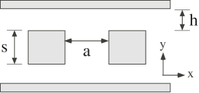
Figure 1: Schematic of a two-dimensional geometry: two metal squares $s\times s$ separated by a distance $a$, and separated from two adjacent metal sidewalls by a a distance $h$.

The ray optics approximation expresses the Casimir force in terms of a sum of contributions from all possible classical ray paths (loops) with the same starting and ending point Jaffe04 . While it is strictly valid only in the limit of low surface curvature, since it neglects diffraction effects, the rays include multiple-body interactions because there exist loops that bounce off multiple objects. In contrast, most other low-curvature approximations, such as PFA bordag01 or other perturbative expansions Sedmik06 ; Schaden98 , are essentially pairwise-interaction laws, and can therefore miss interesting physics that occurs when multiple bodies are brought together. One example occurs in the structure depicted in Fig. 1, where there is a force between two square ($s\times s$) metallic blocks separated by a distance $a$ that is affected by the presence of two infinite parallel metallic sidewalls, separated from the blocks by a distance $h$. For perfect metals in the $h=0$ limit, this geometry was solved analytically in both two dimensions Cavalcanti04 for Dirichlet boundary conditions and in three dimensions Hertzberg07 ; Marachevsky07 for electromagnetic fields. (By “two dimensions,” we mean three-dimensional electromagnetism restricted to $z$-invariant fields; equivalently, a combination of scalar waves with Dirichlet and Neumann boundary conditions, corresponding to the two polarizations.) For $h>0$, this geometry was recently solved by an exact computational method (that is, with no uncontrolled approximations) based on numerical evaluation of the electromagnetic stress tensor Rodriguez07:PRL ; Rodriguez07:PRA . In this case, an unusual effect was observed: as $h$ is increased from $0$, the force between the blocks varies non-monotonically with $h$. The attractive force between the squares actually decreases with $h$ down to some minimum and then increases toward the asymptotic limit of two isolated squares $h\rightarrow\infty$. In the numerical solution, this non-monotonic effect arose as a competition between the TM polarization (electric field in the $z$ direction, with Dirichlet boundary conditions) and the TE polarization (magnetic field in the $z$ direction, with Neumann boundary conditions), which have opposite dependence on $h$. As explained below, it is unclear how this non-monotonic effect could arise in PFA or similar methods—even if sidewall effects are included by restricting the pairwise force due to line-of-sight interactions, it seems that the effect of the sidewall must always decrease monotonically with $h$. When we analyze this structure in the ray-optics approximation, however, we find that a similar competition between the loops with an even and odd number of reflections again gives rise to a non-monotonic $h$ dependence.

Below, we first give a general outline of the ray-optics approach, explain why pairwise approximations such as PFA must fail qualitatively in this geometry, and then present our results for the structure of Fig. 1 in two dimensions. This is followed by a detailed description of the ray-optics analysis for this structure, which involves a combination of analytical results for certain (even-reflection) paths and a numerical summation for other paths.

II Ray-optics Casimir forces

Following the framework of Jaffe04 , we express the two-dimensional Casimir energy via the ray-optics approximation. The ray-optics approach recasts the Casimir energy as the trace of the (scalar) electromagnetic Green’s function $G(\mathbf{x},\mathbf{x}^{\prime})=[\nabla^{2}-\omega^{2}\varepsilon(\mathbf{x},\omega)]^{-1}\delta(\mathbf{x}-\mathbf{x}^{\prime})$, which is in turn expressed as a sum over contributions from classical “optical” paths via saddle-point integration of the corresponding path-integral (this is also referred to as the “classical optical approximation”). The optical paths follow straight lines and are labeled by the number of specular reflections from the surfaces of the conducting objects. In particular, the Casimir energy between flat surfaces for Dirichlet ($\eta=-1$) or Neumann ($\eta=1$) boundary conditions is given approximately by Jaffe04 :

$$\mathcal{E}_{r}=-\frac{\hbar c}{4\pi}\sum_{r}\eta^{r}\int_{D_{r}}\frac{d^{2}x}{\ell_{r}(\mathbf{x})^{3}}$$ (1)

Here, the length of a closed geometric path starting and ending at a point $\mathbf{x}$ is denoted by $\ell_{r}(\mathbf{x})$. $D_{r}$ is the set of points that contribute to a closed optical path reflecting $r$ times from the conducting surfaces. The Casimir energy above is thus the integral over the whole domain of such points. This problem reduces to computing a term-by-term contribution from each possible closed path, as determined by the specific geometrical features of the system under consideration. Because the Neumann (TE) and Dirichlet (TM) boundary conditions are given by the sum and difference of the even and odd paths (paths with even/odd numbers $r$ of reflections), respectively, it is convenient to compute the contribution of even and odd paths separately. The Casimir force is then obtained by the derivative of the energy with respect to the object separation $a$.

Equation 1 is exact for objects with zero curvature (flat surfaces). In the presence of curved surfaces (or sharp corners, which in general have measure-zero contribution to the set of ray paths), however, the energy will include additional diffractive effects that are not taken into account by Eq. 1. One can include low-order corrections for small curvature Jaffe04:preprint , but this is obviously not applicable to the case of sharp corners. There is one special exception, the $h=0$ “piston”: in this case, the sum over optical paths reduces to the method of images, which is exact for the interior of rectangular structures. These limitations are to be expected, however, since the optical theorem is a stationary-phase approximation.

III Pairwise-interaction approximations

There are various pairwise-interaction force laws that have been proposed as approximate methods to compute Casimir forces in arbitrary geometries. The most well-known of these is the proximity-force approximation (PFA), which treats the force between two bodies as a pairwise sum of “parallel-plate” contributions bordag01 . PFA is exact for parallel plates, and may have low-order corrections for small curvature Bordag06 , but is an uncontrolled approximation for strong curvature where it can sometimes give qualitatively incorrect results emig01 ; genet03 ; emig03_1 ; gies06:PFA ; maianeto05 ; Rodriguez07:PRL . Another pairwise interaction is the Casimir-Polder $1/r^{7}$ potential, valid in the limit of dilute media, which has recently been proposed as a simple (uncontrolled) approximation for arbitrary geometries by renormalizing it for the parallel-plate case Casimir48:polder ; Sedmik06 . In this section, we briefly argue why no such pairwise-interaction approximation can give rise to the non-monotonic dependence on $h$ that we observe in the structure of Fig. 1.

Of course, if one considers the pairwise interaction as a true two-body force, for each pair of bodies in isolation, then the sidewalls in the structure can have no effect whatsoever: the force from one sidewall on one square will be exactly vertical (and cancelled by the force from the other sidewall). However, a “lateral force” from the sidewalls, or equivalently an $h$-dependent change in the attractive force between the two squares, can be obtained by restricting the pairwise interactions to “line of sight” forces. For example, when considering the force on one vertical edge of a square from one of the sidewalls, one would include contributions only from the portion of the sidewall that is “visible” from that edge (connected in a straight line from a point on the edge to the point on the sidewall without passing through either square) . For a fixed $h$, the line-of-sight force on the left edge of a square will be different from the force on the right edge, since one edge will have a portion of the sidewall blocked by the other square, and hence there will be an $h$-dependence of the horizontal attractive force.

In particular, since the outside edges of the squares “see” (and are attracted to) a greater portion of the sidewalls than the inside edges, the net force from the sidewalls will always reduce the attractive force between the squares. Already, this contradicts the exact numerical calculations, in which both the Neumann force and the total force are greater at $h=0$ than for $h\rightarrow\infty$.

Moreover, the effect of the sidewalls in a pairwise approximation must always decrease with $h$, again contradicting our results and making non-monotonic effects impossible. As $h$ increases, two things happen: first, the inner edges of the square “see” a larger portion of the sidewalls, with area proportional to $h$; second, the distance from the sidewalls to the squares increases proportional to $h$. The latter contribution must always dominate, however, because any pairwise force must decrease at least as fast as $1/h^{3}$ in two dimensions in order to reproduce the parallel-plate result. Therefore, the sidewall contribution must decrease monotonically at least as fast as $1/h^{2}$ in any pairwise-interaction approximation.

Unlike pairwise-interaction approximations, we show below that the ray-optics approximation correctly reproduces both qualitative behaviors: the total force is larger for $h=0$ than for $h\rightarrow\infty$, and the total force is non-monotonic in $h$.

IV Results

Here, we present the results of our calculations for the general $h\geq 0$ structure shown in Fig. 1, and compare with the numerical results from the stress-tensor method Rodriguez07:PRL ; Rodriguez07:PRA . It turns out that the ray-optics technique indeed captures the non-monotonic dependence of the force with $h$, although of course the quantitative predictions differ from the exact calculations. By definition of ray optics, these quantitative corrections can be attributed to diffraction from the corners. Because we wish to emphasize the results of the ray-optics approach, rather than the details of the calculation of the different loop-lengths $\ell_{r}$ in Eq. 1, we defer those calculational details until Sec. V and here discuss the results.

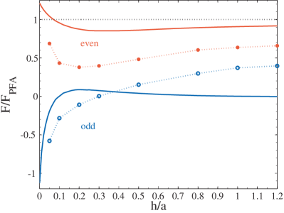
Figure 2: Casimir even (red) and odd (blue) forces vs. sidewall separation $h$ normalized by the the PFA force $F_{\text{PFA}}=-\hbar c\zeta(3)s/8\pi a^{3}$ (dashed black), computed using the ray-optics (solid) and stress-tensor (dashed) methods. Note that the ray-optics results become exact as $h\rightarrow 0$.

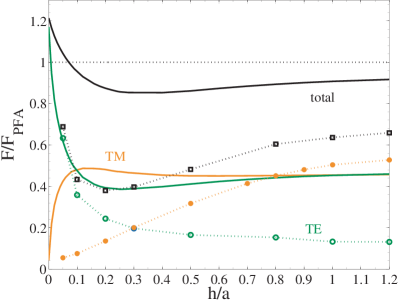
Figure 3: Casimir force vs. sidewall separation $h$ normalized by the the PFA force $F_{\text{PFA}}=-\hbar c\zeta(3)s/8\pi a^{3}$, computed using the ray-optics (solid) and stress-tensor (dashed) methods. The Neumann (green), Dirichlet (orange) and total (black) forces are all normalized by the total Neumann+Dirichlet PFA force.

Figures 2 and 3 show two different plots of the force vs. distance from the metal sidewalls $h$, computed via both Eq. 1 (solids) and the numerical stress-tensor method (dashed). All results are normalized by the PFA force between isolated squares (see captions), which are independent of $h$. The bottom panel shows the contributions from Neumann boundaries (TE polarization) and Dirichlet boundaries (TM polarization), along with the total Neumann+Dirichlet force. Recall that, in the ray optics approximation, the Neumann/Dirichlet forces are given in terms of the even- and odd-path contributions by $(\mathrm{even}\pm\mathrm{odd})/2$, respectively, and thus the total Neumann+Dirichlet force is equal to the contribution of the even paths alone. Because the even/odd decomposition is more natural, in the ray optics approximation, than Neumann/Dirichlet, the top panel shows the even/odd contributions from the same calculations. (Although the stress-tensor calculation does not decompose naturally into even and odd “reflection” contributions, here we simply define the even/odd components as $(\mathrm{Neumann}\pm\mathrm{Dirichlet})/2$, respectively.)

As $h$ goes to zero, the ray-optics results become exact. The numerical computation of the stress-tensor force becomes difficult for small $h$ due to our implementation’s uniform grid, but nevertheless the linear extrapolation of the numerical calculations to $h=0$ agree with ray optics to within a few percent. For $h>0$, the total force for both the ray-optics and stress-tensor results displays a minimum in the range $h\sim 0.2$–$0.3$. In particular, the extrema lie at $h\approx 0.3$ and $h\approx 0.25$, respectively. Not only is this striking non-monotonic behavior captured by the ray-optics approximation, but the agreement in the location of the extremum is also excellent.

Thus far, Figs. 2 and 3 reveal two significant differences between the ray-optics and stress-tensor results. First, the forces when $h$ is not small differ quantitatively, by about 30% as $h\rightarrow\infty$. Since the ray-optics approximation is essentially obtained by dropping terms due to diffraction (from curved surfaces and corners), we can attribute this quantitative difference to the diffractive contribution to the Casimir force from the finite size. In the large-$h$ limit, where the sidewalls become irrelevant and the ray-optics result approaches PFA, the differences compared to the exact solution are sometimes called edge effects Rodriguez07:PRL ; Rodriguez07:PRA ; gies06:edge . Second, although the exact and ray-optics results match in the $h=0$ limit as discussed above, the functional forms for small $h$ are quite different, at least for Dirichlet boundaries. In the ray optics expressions, the odd contributions have a logarithmic singularity at $h=0$, which lead to corresponding singularities in the Neumann and Dirichlet forces. However, in the exact stress-tensor calculation, only the Neumann force seems to display a sharp upturn in slope as $h=0$ is approached (although it is impossible to tell whether it is truly singular); the stress-tensor Dirichlet force seems to be approaching a constant slope (which is why we were able to linearly extrapolate it to $h=0$ with good accuracy).

Another qualitative difference appears if we look at the even and odd contributions in Fig. 2: whereas ray optics and the stress-tensor method give a similar non-monotonic shape for the even force, the odd forces are quite different. (The stress-tensor odd force is monotonic while the ray-optics odd force is not, while the latter goes to zero for large $h$ and the former does not.) Again, we attribute this to a greater sensitivity to diffraction effects, this time for the odd forces compared to the even forces. As will be argued in Sec. V.1, the domain of integration and the length of even ray-optics paths have a weaker dependence on the corners of the squares than the odd paths, and thus should be less sensitive to corner-based diffractive effects. Fortunately, the total force depends solely on the even path contributions, which helps to explain why ray-optics ultimately does effectively capture the non-monotonic behavior and the location of the extremum.

Having explored the $h$-dependence of the force using both ray-optics and numerical stress-tensor methods, we now turn to Fig. 4 to study the behavior of the force as a function of the square separation $a$. Figure 4 shows the Casimir force vs. square separation $a$ at constant $h/s=0.25$, normalized by the PFA force between isolated squares (top panel) or by the exact force at $h=0$ (bottom panel). Note that in both cases the normalization is $a$-dependent, unlike in Figs. 2 and 3, and any non-monotonicity in Fig. 4 is only an artifact of this normalization. The normalization by the PFA force allows us to gauge both the sidewall/edge effects (which disappear for $a\rightarrow 0$) and whether there is a difference in scaling from PFA’s $1/a^{3}$ dependence. For the bottom panel, we normalize against the exact $h=0$ force, which tells us whether the finite sidewall separation makes a difference for the large-$a$ scaling. In both cases, we show a few points of the stress-tensor calculation (which became very expensive for small or large $a$), to get a sense of the accuracy of the ray-optics method at different $a$.

We should expect that as $a\rightarrow 0$, both the PFA and the ray-optics solution should approach the exact solution, because the sidewall contribution becomes negligible. This agreement, as compared to the extrapolated numerical stress-tensor results, can be observed in Fig. 4(top). In contrast, for the large-$a$ limit the ray-optics force appears to decay as $1/a^{2}$ instead of $1/a^{3}$ for PFA, leading to the apparent linear growth in the top panel of Fig. 4. If we compare to the $h=0$ dependence in Fig. 4(bottom), it appears to be asymptoting to a constant for large $a$, indicating that the power laws for $h=0$ and $h>0$ may be identical. However, even if we had more data it would be difficult to distinguish the presence of, for example, logarithmic factors in this dependence. For the $h=0$ case, we have analytical results for even- and odd-path forces in Sec. V.3: from the analytical expressions, the odd-path $h=0$ force clearly goes as $1/a^{2}$, and the even-path $h=0$ force also turns out to have the same $1/a^{2}$ dependence . The exact stress-tensor computation appears to be quite different from both the PFA and the ray-optics force as a function of $a$, but we were not able to go to large enough computational cells to estimate the asymptotic power law. It is striking that $h/s$ as small as $0.25$ is already large enough to yield substantial diffraction effects in the force.

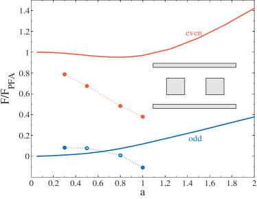
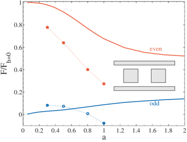
Figure 4: Casimir force vs. separation between squares $a$ with constant sidewall separation $h=0.25$, normalized by the $F_{\text{PFA}}=-\hbar c\zeta(3)s/8\pi a^{3}$ (top) and the corresponding $h=0$ force (bottom). The force is computed for both even (red) and odd (blue) contributions, separately. Inset: schematic of geometry consisting of two isolated squares with adjacent sidewalls.

V Details of the ray-optics computation

In this section, we describe the computation of the ray-optics approximation for the $h>0$ squares+sidewalls structure, according to Eq. 1. This involves systematically identifying all of the possible closed ray loops, integrating them for a given number of reflections over the spatial domain, and then summing over the number of reflections. It turns out that the contributions of any even reflection order can be integrated analytically as shown below, although the final summation over reflection order is still numerical. On the other hand, the integrals from the odd reflection orders become increasingly difficult as the reflection order is increased, and so we resorted to numerical integration for odd orders $r>5$.

V.1 Even paths

Because we are dealing with perfect metals, and because the geometry has reflection-symmetry about the $x$ and $y$ axes, it is helpful to represent the optical paths using an infinite periodic lattice, shown in Fig. 5, similar to the construction in Hertzberg07 . The reason for this construction is that, because of the equal-angle law for specular reflections in geometric optics, a reflected ray is equivalent to a linearly extended ray in a mirror-image structure. This allows us to visualize and count the set of possible closed paths in a straightforward fashion. Specifically, a closed path which starts at a point $\mathbf{x}$ and ends on itself is fully determined by the set of lines that start at $\mathbf{x}$ and end in the corresponding set of image points on the extended lattice. The unit cell of this periodic construction is just two vertical black lines (of length $s$ and separation $a$) that represent the parallel walls of the two squares. These are repeated with a horizontal period $a$ and a vertical period $s+2h$. Any path that passes through the gap between one of these lines and the horizontal sidewalls escapes from between the two squares and therefore is not counted among the closed loops.

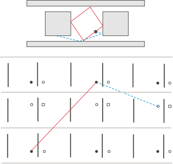
Figure 5: Schematic of general 2d squares+sidewalls lattice. Lines extending from solid circles unto solid circles represent even reflection paths. Lines extending from open solid circles unto open circles represent odd reflection paths. (Here, $h/a\approx 0.2$ and $s/a\approx 1$.) A possible even (red) and forbidden odd (blue) path is shown.

In order to construct all of the closed loops that originate at a given point $\mathbf{x}$ in the unit cell, we proceed as follows. First, we construct the mirror reflections of this point through the vertical lines (the boundaries of the squares) and the horizontal lines (the sidewalls), corresponding to reflections from these metallic walls. This gives us a set of points in the nearest-neighbor cells. Then, we construct the reflections of the nearest-neighbor points through their sidewalls, and so on, corresponding to reflections of higher and higher order. A closed loop is simply a line segment from the original $\mathbf{x}$ to one of the reflected points, as long as it does not escape through one of the gaps between the squares and sidewalls as explained above. Figure 5 was generated from a unit cell with $h/a\approx 0.2$ and $s/a\approx 1$, and shows both even-reflection (solid red) and odd-reflection (dashed blue) paths, where in this case the odd path shown escapes and therefore would not be counted. In the figure, the points are labelled according to the number of reflections that generate them from the original point: solid circles when the numbers of horizontal and vertical reflections are both even, open squares when the numbers are both odd, and open circles otherwise. It follows that lines connecting solid circles to solid circles are even paths, and lines connecting solid to open circles are odd paths; the rays connecting solid circles and squares always escape and therefore do not contribute..

To compute the Casimir energy from these paths, the key quantity in Eq. 1 is the length $\ell$ of the path. Let us label each unit cell by $(n,m)$ according to its horizontal ($n$) and vertical ($m$) offset from the cell $(0,0)$ where the original point $\mathbf{x}$ resides. For an even path, $\mathbf{x}$ must be connected to an even-indexed image $(2n,2m)$, for which the length of the path is:

$$\ell_{n,m}=\sqrt{(2na)^{2}+\left[2m\left(2h+s\right)\right]^{2}}$$ (2)

and the angle of the path, determined by $m/n$, is:

$$\tan\theta_{n,m}=\frac{m}{n}\frac{2h+s}{a}.$$ (3)

The only things left to figure out are the domain of integration of $\mathbf{x}$ and the allowed $(n,m)$ for non-escaping paths. If $h=0$, it is obvious that our expression reduces to the expression of Hertzberg07 , since both the whole spatial domain within the unit cell and all $(n,m)$ are allowed. However, when $h>0$, each $(n,m)$ will be non-escaping only for $\mathbf{x}$ in a subset of the unit cell. To determine these subsets, the domains of integration, we take advantage of the closed-loop nature of the paths to cast Eq. 1 in a different light. For a given $(n,m)$, instead of integrating over $x$ and $y$, it is convenient to change variables to integrate over $y$ and a coordinate $\xi=x/\cos\theta_{n,m}$ measuring displacement along the path (along the $\theta_{n,m}$ direction). It might seem that one should integrate $\xi$ along the whole line from $(0,0)$ to $(n,m)$, but this may involve counting the same point $\mathbf{x}$ in the unit cell multiple times. Instead, to avoid over-counting loops that wrap around on themselves, one instead integrates from $(0,0)$ to $(\tilde{n},\tilde{m})$ where $\tilde{n}=n/\gcd(n,m)$ and $\tilde{m}=m/\gcd(n,m)$ are reduced to lowest terms. One then obtains the following equation for the energy:

$$\mathcal{E}_{\mathrm{even}}=-\frac{\hbar c}{4\pi}\sum_{n,m}\int dy\int_{\xi(0,0)}^{\xi(\tilde{n},\tilde{m})}d\xi\cos\theta^{\prime}_{\tilde{n},\tilde{m}}\frac{1}{\ell^{3}_{n,m}}$$ (4)

Although not so obvious from looking at Eq. 4, the integral in the $y$ direction simply counts the number of $(\tilde{n},\tilde{m})$ paths that exist in the unit cell. Because the length and angle of such paths are independent of $y$, we can integrate over $d\xi$ to obtain:

$$\mathcal{E}_{\mathrm{even}}=-\frac{\hbar c}{4\pi}\sum_{n,m}\int dy\frac{2\tilde{n}a}{\ell^{3}_{n,m}}$$ (5)

where we used $\int d\xi=\ell_{\tilde{n},\tilde{m}}$ and $\cos\theta_{\tilde{n},\tilde{m}}=2\tilde{n}a/\ell_{\tilde{n},\tilde{m}}$, between which the $\ell_{\tilde{n},\tilde{m}}$ cancels. All that is left to figure out is the integral in the $y$ direction.

To carry the integral in the $y$ direction, we must determine the limits of integration, or equivalently, the range over which we can displace the path so that it does not escape. We go back to Fig. 5 for reference. Again, as outlined above, we extend a line from a solid circle in the $(0,0)$ cell to another solid circle in the $(2n,2m)$-th cell. For the path to be allowed, it must intercept all of the vertical black line segments that lie between the two points, i.e. at each horizontal reflection from the squares. Because each interception (horizontal reflection) occurs at periodic intervals, these end up partitioning the unit cell in the $y$ direction into $\tilde{n}$ sets of length $(2h+s)/\tilde{n}$. Note that that we divide by $\tilde{n}$, rather than $n$, because as explained above the topologically distinct paths are uniquely specified by $(n,m)$ reduced to lowest terms. From this simple argument, we obtain that the vertical displacement is $(2h+s)/\tilde{n}-2h$, provided that $(2h+s)/\tilde{n}-2h>0$. To help visualize this result, it is best to think of the problem on a circle. That is, consider a circle of length $2h+s$ and partition it into $\tilde{n}$ sets of length $(2h+s)/\tilde{n}$, as well as into two regions of length $s$ and $2h$. If the path is to exist, each of the $(2h+s)/\tilde{n}$ points on the circle must not intercept the region marked as belonging to $2h$ (the air gaps between the squares). The result follows directly by considering the distance that one can displace the points before any of them intercepts the $2h$ region.

Thus, the final expression for the even path energies is left as a sum over $n$ and $m$:

$$\mathcal{E}_{\mathrm{even}}=-\frac{\hbar c}{4\pi}\sum_{n,m>0}\Theta\left(\frac{2h+s}{\tilde{n}}-2h\right)\left[\frac{2h+s}{\tilde{n}}-2h\right]\frac{4\tilde{n}a}{\left[(2na)^{2}+(2m(2h+s))^{2}\right]^{3/2}}$$ (6)

An extra factor of 2 was included in the numerator since the contributions of the $(-n,-m)$ paths are identical to those of the $(n,m)$ paths by symmetry. In the limit $h=0$, we recover the even energy expression of Hertzberg07:notes , given in Sec. V.3.

Although we are almost done with the even reflection paths, we are missing a very important contribution to the energy: the PFA terms, i.e. the $(n,0)$ and $(0,m)$ paths. The PFA energy between two parallel finite metal regions is a well-known result, and we include here only $(n,0)$ for completeness:

$$\mathcal{E}_{\mathrm{PFA}} = -\frac{\hbar csa}{16\pi}\sum_{n>0}\frac{1}{(na)^{3}}$$ (7)

$$= -\frac{\hbar cs\zeta(3)}{16\pi a^{2}}$$

The final expression Eq. 6 must still be summed numerically over $(n,m)$ up to some upper cutoff, but this is an simple computation and its convergence with the cutoff is discussed in Sec. V.4.

V.2 Odd paths

Unlike even reflections, odd reflection paths are quite tedious to compute because have less symmetry. For one thing, the length of a path depends not only on $(n,m)$ (the offset of the unit cells being connected), but also on the position $\mathbf{x}$ of the starting point. More importantly, the identification of the domain of $\mathbf{x}$ for non-escaping paths depends in a much more complicated way on $(n,m)$, making it difficult to write down a single expression that works for all $(n,m)$. Therefore, we analytically solved for the odd-path contributions only up to five-reflection paths, where each order requires a separate analysis, and treated higher-order paths by a purely numerical approach. Below, the analytical solution for the third-order paths is given, both to illustrate the types of computations that are involved and also to demonstrate the logarithmic singularity in the force as $h\rightarrow 0$.

The results of Hertzberg07 give an upper limit for the number of odd paths $r\geq 3$ that exist in this geometry for $h=0$ (# paths = $2^{(r+3)/2}$). The same upper limit holds for $h>0$, but in this case the number of paths is actually reduced because some of the $h=0$ paths now escape. An analytical solution for any particular order must begin by drawing all paths for $h=0$ and then perturbing them for $h>0$ to eliminate any impossible paths. At least for low-order paths, simple geometrical arguments can then determine the domain of integration.

The coordinate dependence of odd paths arises from the fact that any path that reflects an odd number of times from the planar surfaces will be non-periodic: if we extend the path beyond its endpoint (= starting point), it will not repeat. This greatly complicates the analysis. For example, Fig. 5 shows one such escaping odd path. It turns out that as $h$ grows, the domain of integration for odd paths shrinks and becomes harder to visualize. Moreover, if we vary $h$, we notice that paths for some $(n,m)$, regardless of their origin $\mathbf{x}$, always escape. The problem of determining the domain of integration and the allowed $(n,m)$ seems rather difficult and does not seem to have a general closed-form solution.

V.2.1 Three-reflection paths

From Fig. 5 we verify that there are eight possible three reflection paths, $(\pm 2,\pm 1)$ and $(\pm 1,\pm 2)$ according to the notation of Sec. V.1, shown in Fig. 6. The only two nonequivalent cases are $(2,1)$ and $(1,2)$, which have different domains of $\mathbf{x}$ integration.

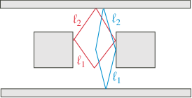
Figure 6: Schematic of three-reflection paths. Blue/red represent $(1,2)$/$(2,1)$ paths, and the lengths $\ell_{i}$ shown are used the calculation of the energy.

Inspection of Fig. 6 and Fig. 5 yields the length of these paths $\ell_{2,1}=2\sqrt{a^{2}+\left(2h+s-y\right)^{2}}$. Moreover, we see that $\ell_{2,1}$ is invariant along the $x$-axis. For this particular path, the maximum displacement in the vertical direction $y_{\textrm{max}}$ occurs when $\ell_{1}\sin\theta=\ell_{2}\sin\theta=h$, while the minimum $x_{\textrm{min}}$ and maximum $x_{\textrm{max}}$ horizontal displacements occur when $\ell_{2}\sin\theta=h$ and $\ell_{1}\sin\theta=h$, respectively. Therefore, the range of integration is:

$$0\leq y \leq s$$ (8)

$$\left(\frac{ah}{2h+s-y}\right)\leq x \leq\frac{a(h+s-y)}{2h+s-y},$$ (9)

giving us the following expression for the energy:

$$\mathcal{E}_{2,1}=-\frac{\hbar c}{32\pi a^{2}}\left\{\frac{sa}{\sqrt{a^{2}+\left(2h+s\right)^{2}}}\right.\\ \left.-2h\log\left[\left(\frac{2h+s}{2h}\right)\frac{1+\sqrt{1+\left(\frac{2h}{a}\right)^{2}}}{1+\sqrt{1+\left(\frac{2h+s}{a}\right)^{2}}}\right]\right\}.$$ (10)

In order to compute $\mathcal{E}_{1,2}$, we apply similar geometrical considerations. Once again, from Fig. 5 we obtain the length to be $\ell_{1,2}=2\sqrt{\left(a-x\right)^{2}+\left(2h+s\right)^{2}}$. Similarly, we see that $\ell_{1,2}$ is invariant along $y$-axis, and approaches a minimum when $x=a$. Therefore, the range of integration is:

$$h\leq y \leq h+s$$ (11)

$$0\leq x \leq a,$$ (12)

giving us the following expression for the energy:

$$\mathcal{E}_{1,2}=-\frac{\hbar cas}{32\pi\left(2h+s\right)^{2}}\frac{1}{\sqrt{a^{2}+\left(2h+s\right)^{2}}}.$$ (13)

Adding Eq. 10 to Eq. 13, and multiplying by four to account for the different $\pm$ sign possibilities in $(n,m)$ yields the total three-reflection contribution to the energy. This contribution has two types of terms: a polynomial term from Eq. 13 and the first term of Eq. 10, and a logarithmic term from the second term of Eq. 10. The polynomial term remains at $h=0$. The more intriguing component of this result is the logarithmic term, which falls as $O(h\log h)$ for small $h$, vanishing completely at $h=0$. This (and similar terms for higher-order reflections) is the source of the logarithmic singularity in slope of the ray-optics odd-path Casimir force at $h=0$ observed in Fig. 2.

V.2.2 Five-reflection paths

The analytical solution of the five-reflection contribution is rather complicated and is not reproduced here. However, it has a few interesting features that we summarize here. First, just as for the three-reflection paths, the five-reflection contribution has an $O(h\log h)$ term that contributes to the singularity we observe in the ray-optics odd-path Casimir force at $h=0$. Second, one also obtains $O(\log h)$ terms, which should seem to unphysically diverge as $h\rightarrow 0$. It turns out, however, that for a path that gives a $(\log h)$ contribution at small $h$, there exists another path with a $-(\log h)$ contribution, resulting in exact cancellation of any divergences.

V.3 Casimir piston

The $h=0$ limit is the well-known “Casimir piston” geometry. In this limit, all of the optical paths contribute to the Casimir energy, making it possible to compute Eq. 1 analytically. Hertzberg07 performs this calculation in three-dimensions, and a similar unpublished result was obtained in two-dimensions Hertzberg07:notes . The two-dimensional geometry was also solved analytically for Dirichlet boundaries by another method Cavalcanti04 . Here, we reproduce this calculation as a check on both the even- [Eq. 6] and odd-path [Eqs. 13 and  10] contributions to the energy, and also because the Neumann result is useful and previously unpublished.

We begin by computing the $h=0$ even-path contributions. The expression for the even energy Eq. 6 is much simpler than for $h>0$, because the $\Theta$ function disappears and all that is left is a polynomial function in terms of $n,m$. The even-path energy, not including the PFA contribution (terms where $n=0$ or $m=0$, but not both), is given by:

$$\mathcal{E}_{\mathrm{even}} = -\frac{\hbar c}{8\pi}\sum_{n,m>0}as\left(\left(na\right)^{2}+\left(ms\right)^{2}\right)^{-3/2}$$ (14)

$$= -\frac{\hbar c}{8\pi}as\textrm{Z}_{2}(a,s;3)$$ (15)

we have identified the summation above as the second order Epstein Zeta function $\textrm{Z}_{2}$:

$$\textrm{Z}_{2}(a,b;p)=\sum_{n,m>0}\left((na)^{2}+(mb)^{2}\right)^{-p/2}$$ (16)

The same simplification occurs in the case of odd paths, the lengths of which can be found, again, by inspection of the lattice in Fig. 5. Again, as described in Sec. V.1, given a point on the unit cell $\mathbf{x}$, one can determine all possible odd-reflection paths by drawing straight lines from the solid circles ($\mathbf{x}$) to the open circles in the lattice.

There are two types of open circles, each of which denote two different types of paths: those that reflect across the $x$ axis and have $y$-invariant length, as well as those that reflect across the $y$ axis and have $x$-invariant length. Whichever coordinate is the invariant one gives a constant integral over the unit cell, so the double integral is reduced to a single integral. For example, consider those that reflect across the $x$ axis and have $y$-invariant length: for these paths, we need to integrate over $x$ in the unit cell and perform a double sum over $(n,m)$. However, the double sum can be reduced to a single sum by eliminating the sum over $n$ in favor of integrating $x$ along the whole real line instead of just the unit cell. Thus, we are left with a single integral and a single summation. Similarly paths that reflect across the $y$ axis reduce to a single integral over $y$ and a single sum over $n$. As a result of all this manipulation, the odd integral becomes:

$$\mathcal{E}_{odd}=-\frac{\hbar cs}{32\pi}\sum_{m>0}\int_{-\infty}^{\infty}\frac{dx}{[(ms)^{2}+x^{2}]^{3/2}}\\ -\frac{\hbar ca}{32\pi}\sum_{n>0}\int_{-\infty}^{\infty}\frac{dy}{[(na)^{2}+y^{2}]^{3/2}}.$$ (17)

Again, we restrict the sum to $n,m>0$, because horizontal and vertical paths are divergent terms that contribute only to the self-energy of the metallic walls Jaffe04:preprint . Carrying out the above integrals yields the following expression for the odd-path energy:

$$\mathcal{E}_{\text{odd}}=-\frac{\hbar c\pi}{48}\left(\frac{1}{s}+\frac{1}{a}\right).$$ (18)

The odd-path contribution to the force is therefore $\propto 1/a^{2}$ for large $a$.

V.4 Numerics

To evaluate Eq. 1 numerically, we used an adaptive two-dimensional quadrature (cubature) algorithm Genz83 to perform the $\mathbf{x}=(x,y)$ integration for each $(n,m)$. (For each $\mathbf{x}$ and $(n,m)$ it is easy to numerically check whether the path is allowed, and set the integrand to zero otherwise. Unfortunately, this makes the integrand discontinuous and greatly reduces the efficiency of high-order quadrature schemes; an adaptive trapezoidal rule might have worked just as well. For very small $h$, this requires some care because the energy depends on a tiny remainder between two diverging terms, as we saw in Sec. V.2.2, but for most $h$ there was no difficulty.

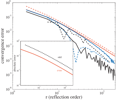
Figure 7: (Color:) Convergence error $(\mathcal{E}_{r+1}-\mathcal{E}_{r})/\mathcal{E}_{r}$ in the even (solid) and odd (dashed) path contributions vs. reflection order $r$ for values of $h=0$ (red), $h=0.01$ (blue), and $h=0.1$ (black) (here, $\mathcal{E}_{r}$ means the energy computed up to order $r$). Inset: Absolute error $(\mathcal{E}_{\text{exact}}-\mathcal{E}_{r})/\mathcal{E}_{\text{exact}}$ for both even (solid black) and odd (dashed red) contributions for $h=0$.

We repeat this calculation for increasing reflection order $r$ until the total energy $\mathcal{E}_{r}$ converges to the desired accuracy. From general considerations, one expects the error $|\mathcal{E}-\mathcal{E}_{r}|$ for the energy from a finite $r$ to decrease as $O(1/r)$. In particular, the path lengths $\ell$ increase proportional to $r$ (the radius in the extended lattice), and the number of paths with a given length also increase proportional to $r$ (the circumference in the extended lattice), so the $\sum 1/\ell^{3}$ for a given $r$ goes as $O(1/r^{2})$. The error in the energy is the sum over all paths of order $>r$, and this therefore goes as $O(1/r)$. This scaling is verified in Fig. 7, which plots the relative error $(\mathcal{E}_{r+1}-\mathcal{E}_{r})/\mathcal{E}_{r}$ between the order-$r$ and the order-$(r+1)$ energy computations for the particular case of $a=s=1$. In general, if the energy converged as $O(1/r^{n})$ for some power $n$, one would expect this difference to converge as $O(1/r^{n+1})$, and so we expect Fig. 7 to asymptotically go as $O(1/r^{2})$. This is precisely what is observed, for both even and odd paths, and for both $h=0$ and $h>0$: all of the curves asymptotically approach straight lines (on a log–log scale) with slope $-2$.

An interesting though unfortunate result is that the odd-path energy requires larger $r$ in order to obtain the same accuracy as the even-path energy. Though this may not be obvious from looking at the convergence error, it is clear from the inset of Fig. 7, where we plot the absolute error $(\mathcal{E}_{\text{exact}}-\mathcal{E}_{r})/\mathcal{E}_{\text{exact}}$ instead (at $h=0$). The constant offset observed in the absolute errors imply that, given a desired accuracy constrain on the even and odd energy calculations, one would have to compute roughly twice the number of odd paths in order to obtain equivalent accuracy.

VI Concluding Remarks

By comparing the ray-optics approximation with an exact brute-force calculation, we have been able to study both the successes and limitations of the ray-optics approximation. On the positive side, the ray-optics approximation is capable of capturing surprising behaviors that arise in closed geometries involving multiple bodies, qualitatively matching phenomena identified in exact brute-force calculations. In particular, the ray-optics approximation captures the non-monotonic sidewall effects observed for metallic squares between parallel sidewalls, generalized from the Casimir piston geometry. This effect is clearly a manifestation of the multi-body character of the interaction, since it does not arise in simple two-body force laws such as PFA. Ray optics appears to be unique among the current simple approximations for Casimir force in that it can capture such multi-body effects, even though it cannot be quantitatively accurate in geometries with strong curvature. On the negative side, diffractive effects set in rather quickly when $h$ is increased from zero, marking the agreement between ray-optics and the exact results only qualitative.

This makes the ray optics approximation a promising approach to quickly search for unusual Casimir phenomena in complicated geometries. However, since it is an uncontrolled approximation in the presence of strong curvature, any prediction by ray optics in such circumstances must naturally be checked against more expensive exact calculations. There will undoubtedly be complex structures in the future where ray optics fails qualitatively as well as quantitatively For instance, ray optics has more difficulty with open geometries—e.g., for two squares with only one sidewall, only PFA paths are present. On the other hand, the reach of the ray optics technique seems in some sense to be larger than that of simpler approximations such as PFA.

References

- (1) H. B. G. Casimir, “On the attraction between two perfectly conducting plates,” Proc. K. Ned. Akad. Wet., vol. 51, pp. 793–795, 1948.
- (2) P. W. Milonni, The Quantum Vacuum: An Introduction to Quantum Electrodynamics. San Diego: Academic Press, 1993.
- (3) E. M. Lifshitz and L. P. Pitaevskii, Statistical Physics: Part 2. Oxford: Pergamon, 1980.
- (4) G. Plunien, B. Muller, and W. Greiner, “The Casimir effect,” Phys. Rep., vol. 134, no. 87, 1986.
- (5) V. M. Mostepanenko and N. N. Trunov, The Casimir Effect and its Applications. Oxford: Clarendon Press, 1997.
- (6) S. K. Lamoreaux, “Demonstration of the Casimir force in the 0.6 to 6m range,” Phys. Rev. Lett., vol. 78, p. 5, 1997.
- (7) R. Onofrio, “Casimir forces and non-Newtonian gravitation,” New J. Phys., vol. 8, p. 237, 2006.
- (8) F. Capasso, J. N. Munday, D. Iannuzzi, and H. B. Chan, “Casimir forces and quantum electrodynamical torques: Physics and nanomechanics,” IEEE J. Selected Topics in Quant. Elec., vol. 13, no. 2, pp. 400–415, 2007.
- (9) T. Emig, R. L. Jaffe, M. Kardar, and A. Scardicchio, “Casimir interaction between a plate and a cylinder,” Phys. Rev. Lett., vol. 96, p. 080403, 2006.
- (10) H. Gies and K. Klingmuller, “Casimir edge effects,” Phys. Rev. Lett., vol. 97, p. 220405, 2006.
- (11) A. Rodriguez, M. Ibannescu, D. Iannuzzi, F. Capasso, J. D. Joannopoulos, and S. G. Johnson, “Computation and visualization of Casimir forces in arbitrary geometries: Non-monotonic lateral-wall forces and failure of proximity force approximations,” Phys. Rev. Lett., vol. 99, no. 8, p. 80401, 2007.
- (12) T. Emig, N. Graham, R. L. Jaffe, and M. Kardar, “Casimir forces between arbitrary compact objects,” arXiv.org preprint arxiv, pp. stat–mech–ph/0707.1862, 2007.
- (13) R. L. Jaffe and A. Scardicchio, “Casimir effect and geometric optics,” Phys. Rev. Lett., vol. 92, p. 070402, 2004.
- (14) A. Scardicchio and R. L. Jaffe, “Casimir effects: An optical approach I. foundations and examples,” arXiv.org preprint archive, pp. quant–ph/0406041, 2004.
- (15) M. Bordag, U. Mohideen, and V. M. Mostepanenko, “New developments in the Casimir effect,” Phys. Rep., vol. 353, pp. 1–205, 2001.
- (16) A. Rodriguez, M. Ibannescu, D. Iannuzzi, J. D. Joannopoulos, and S. G. Johnson, “Virtual photons in imaginary time: computing Casimir forces in arbitrary geometries via standard numerical electromagnetism,” Phys. Rev. A, vol. 76, no. 2, p. 093708, 2007.
- (17) M. Hertzberg, “The Casimir piston.” Notes on 2d Casimir piston.
- (18) R. M. Cavalcanti, “Casimir force on a piston,” Phys. Rev. D, vol. 69, p. 065015, 2004.
- (19) R. Sedmik, I. Vasiljevich, and M. Tajmar, “Detailed parametric study of Casimir forces in the Casimir Polder approximation for nontrivial 3d geometries,” J. Computer-Aided Mat. Des., vol. 14, no. 1, pp. 119–132, 2007.
- (20) M. Schaden and L. Spruch, “Infinity-free semiclassical evaluation of Casimir effects,” Phys. Rev. A, vol. 58, pp. 935–953, 1998.
- (21) M. P. Hertzberg, R. L. Jaffe, K. M., and A. Scardicchio, “Casimir forces in a piston geometry at zero and finite temperatures,” arXiv.org preprint arxiv, pp. quant–ph/0705.0139, 2007.
- (22) V. M. Marachevsky, “Casimir interaction of two plates inside a cylinder,” PRD, vol. 75, p. 085019, 2007.
- (23) M. Bordag, “Casimir effect for a sphere and a cylinder in front of a plane and corrections to the proximity force theorem,” Phys. Rev. D, vol. 73, p. 125018, 2006.
- (24) T. Emig, A. Hanke, R. Golestanian, and M. Kardar, “Probing the strong boundary shape dependence of the Casimir force,” Phys. Rev. Lett., vol. 87, p. 260402, 2001.
- (25) C. Genet, A. Lambrecht, P. Maia Neto, and S. Reynaud, “The Casimir force between rough metallic plates,” Europhys. Lett., vol. 62, p. 484, 2003.
- (26) T. Emig, A. Hanke, R. Golestanian, and M. Kardar, “Normal and lateral Casimir forces between deformed plates,” Phys. Rev. A, vol. 67, p. 022114, 2003.
- (27) H. Gies and K. Klingmuller, “Casimir effect for curved geometries: Proximity-force-approximation validity limits,” Phys. Rev. Lett., vol. 96, p. 220401, 2006.
- (28) P. A. Maia Neto, A. Lambrecht, and S. Reynaud, “Roughness correction to the Casimir force: Beyond the proximity force approximation,” Europhys. Lett., vol. 69, p. 924, 2005.
- (29) H. B. G. Casimir and D. Polder, “The influence of retardation on the London-Van der Waals forces,” Phys. Rev., vol. 13, no. 4, pp. 360–372, 1948.
- (30) A. C. Genz and A. A. Malik, “An imbedded family of fully symmetric numerical integration rules,” SIAM J. Numer. Anal., vol. 20, no. 3, pp. 580–588, 1983.