Oscillations of General Relativistic Multi-fluid/Multi-layer Compact Stars
Abstract
We develop the formalism for determining the quasinormal modes of general relativistic multi-fluid compact stars in such a way that the impact of superfluid gap data can be assessed. Our results represent the first attempt to study true multi-layer dynamics, an important step towards considering realistic superfluid/superconducting compact stars. We combine a relativistic model for entrainment with model equations of state that explicity incorporate the symmetry energy. Our analysis emphasises the many different parameters that are required for this kind of modelling, and the fact that standard tabulated equations of state are grossly incomplete in this respect. To make progress, future equations of state need to provide the energy density as a function of the various nucleon number densities, the temperature (i.e. entropy), and the entrainment among the various components.
pacs:
97.60.Jd,26.20.+c,47.75.+f,95.30.SfI Introduction
The fluid approximation Andersson and Comer (2007) is a necessity for modeling systems containing so many elementary constituents that (on a macroscopic scale) they form a continuum, and can redistribute energy and momentum among themselves. The model is based on the notion of fluid element, which is small enough to be infinitesimal with respect to the system , but large enough to contain, say, an Avogadro’s number worth of particles. In a superfluid system one must consider different, dynamically decoupled, yet co-existing fluids. Each individual fluid has its own collection of fluid elements and each spacetime point in the system will have as many fluid element worldlines passing through it as there are independent fluids. The extent to which different fluids are coupled depends largely on the available dissipation mechanisms, eg. friction due to interparticle scattering. In a multi-fluid system this is a complex problem Andersson and Comer (2006). Generally, the system dissipation depends on how energy and momentum are exchanged as the fluid elements expand and contract, how they slide across each other, how they rotate about each other, and how they flow through each other.
Neutron stars are believed to be prime examples of general relativistic, multi-fluid objects. To date, on the order of a couple of thousand pulsars have been observed Lorimer (2005). Yet, an extrapolation of the local population data for our galaxy suggests the existence of about normal pulsars, around millisecond pulsars, and about neutron stars that are no longer active pulsars. Most of these should be extremely cold in the sense that their temperature is several orders of magnitude less than the Fermi temperatures of the independent (massive) particle species, i.e. . In fact, neutron stars cool to temperatures below relatively soon after birth. This is the expected transition temperature Lombardo (1999); Lombardo and Schulze (2001); Andersson et al. (2005) for neutrons and protons to become superfluid and superconducting, respectively. We therefore anticipate that most neutron stars in our galaxy have at least two superfluids/superconductors in their cores. In fact, neutron superfluidity is a key ingredient in most models of large pulsar glitches Radhakrishnan and Manchester (1969); Lyne (1993), with (catastrophic) transfer of angular momentum via vortices from a superfluid component to the crust leading to the observed spin-up.
Ever since neutron star superfluidity was first suggested Migdal (1959), we have seen a concerted effort aimed at developing our understanding of the various phases of matter Lombardo (1999); Lombardo and Schulze (2001); Clark et al. (1992); Glendenning (1997); Walecka (1995). This has led to a picture where a typical neutron star has a number of distinct “layers”. From the outer to the inner crust, protons are locked inside increasingly neutron-rich nuclei which are embedded in a degenerate normal fluid of electrons. At the base of the crust, the nuclei are believed to assume exotic “pasta” shapes Pethick and Ravenhall (1995). Moreover, in the crust region the long-range, attractive component of the nuclear force should lead to Cooper pairing of neutrons in states. The crust nuclei will thus be embedded in and penetrated by superfluid neutrons. Short-range repulsion in the nuclear force and the spin-orbit interaction allow neutrons to pair as states in the more dense regions of the outer core Hoffberg et al. (1970). There are no nuclei in this region and the protons that remain are dilute enough to feel only the long-range attractive part of the nuclear force. Hence, they are expected to pair in states. The core neutrons and protons are embedded in a highly degenerate normal fluid of electrons. At high enough density it becomes energetically favorable for more massive particles to form (eg. muons in lieu of electrons). At the most extreme densities, quarks may become deconfined, possibly opening up a number of channels for attractive interactions and hence many Cooper pairing possibilities (e.g. so-called CFL matter Alford (2004); Alford et al. (2000)). Each individual Cooper pairing will lead to individual condensates, and potentially many inter-penetrating fluids. The actual number of dynamically distinct fluids depends very much on the details of dissipation Andersson and Comer (2006); Gusakov (2007). The scattering time-scale must typically be much greater than the characteristic dynamical time-scales in order for fluid components to decouple.
A moderately realistic neutron star model must account for the presence of different regions in the star. Describing a neutron star as a multi-layer system, one should at the very least account for the presence of the (multi-fluid) superfluid/superconducting regions and the elastic crust component. Even though there has been progress in this area, we are still not at this level of sophistication. The current state-of-the-art is represented by Andersson et al. (2002), where quasinormal modes for a core-envelope model are calculated, and a recent study of axial crust oscillations in the relativistic Cowling approximation Samuelsson and Andersson (2007). The aim of the present work is to improve on the first aspect of the modeling. We will include, for the first time, the physics of the superfluid phase transition in the construction of the spherically symmetric and static background model. The motivation for this is that the different regions of superfluidity may not overlap Andersson et al. (2005), and the fluid dynamics will change depending on whether a given layer is normal or superfluid. This represents an important improvement on previous models, since it allows us to quantify how changes in the superfluid energy gap affect the quasinormal-mode spectrum. We leave inclusion of the crust elasticity for future studies. A fully relativistic formalism for a crust penetrated by a superfluid has been developed, see eg. Carter and Samuelsson (2006), but it is yet to be applied to neutron star dynamics.
In a mixture of the superfluids and , it is known that a momentum induced in one of the constituents will cause some of the mass of the other to be carried along, or entrained Andreev and Bashkin (1975); Vardanyan and Sedrakyan (1981). Another example is the entropy (which can be considered as a massless fluid). In fact, in superfluid the so-called “normal” fluid density is directly proportional to the entrainment between the atoms and the entropy. In a neutron star, the strong interaction leads to entrainment between neutrons and protons. Entrainment is a multi-fluid effect, that has no counterpart in a single-fluid system. When the neutrons start to flow they will, through entrainment, induce a momentum in the protons and subsequently the electrons Alpar et al. (1984). In principle, there could be entrainment between each and every fluid of a multi-fluid system. In this analysis we will only consider the entrainment between neutrons and protons, for which we use the fully relativistic mean field model developed by Comer and Joynt Comer and Joynt (2003).
The outline of this paper is as follows: In Sec. II we give details on the two-fluid formalism, and the set of equations used to model the quasinormal modes. Sec. III discusses an expansion for the local matter content that is adapted to include entrainment at the appropriate order. Sec. IV gives the specifics on the local matter content, i.e. the equation of state, the gap data, and the relativistic entrainment. The following Sec. V provides the results of our analysis of modes for two equations of state, with or without entrainment, and different “temperatures” of the star. Sec. VI gives some concluding remarks and discusses to what extent the extant literature and computational infrastructure for compact object equations of state are adequate for supporting our kind of analysis. Finally, the Appendix describes the technique used to obtain the results in Sec. V. We use “MTW” conventions throughout.
II General Relativistic Two-fluid Formalism
II.1 The full formalism
We will use the formalism developed by Carter, Langlois, and their various collaborators Carter (1989); Comer and Langlois (1993); Comer and Langlois (1994); Carter and Langlois (1995); Langlois et al. (1998); Comer et al. (1999); Prix (2000); Andersson and Comer (2001); Comer (2002); Prix (2004) (see Andersson and Comer Andersson and Comer (2007) for a recent review). The fundamental fluid variables consist of the conserved nucleon density four-currents, to be denoted where is a so-called constituent index (which is not summed over when repeated). From the currents can be formed three scalars: , , and . Given a master function (the two-fluid analog of the equation of state), the stress-energy tensor is
| (1) |
where
| (2) |
is the generalized pressure and
| (3) |
is the chemical potential covector. It is also the momentum canonically conjugate to the current . Formally, the and coefficients are obtained from the master function via the partial derivatives
| (4) |
The fact that the momentum is not simply proportional to the corresponding number density current is a result of entrainment. It vanishes if the coefficient is zero.
Finally, the equations for the neutrons and protons each consist of a conservation equation
| (5) |
and an Euler equation
| (6) |
where the vorticity two-form is defined by
| (7) |
The square brackets indicate antisymmetrization of the enclosed indices. Comer Comer (2002) and Prix et al Prix et al. (2002) discuss in some detail why the assumption of separate conservation laws for the two fluids should be reasonable for slow rotation and quasinormal-mode calculations (excluding the thin transition layers that separate single fluid and multi-fluid layers). Note that the above way of writing the Euler equations makes manifest its geometric meaning as an integrability condition for the vorticity, a point that has been much emphasized by Carter Carter (1989) (see also Andersson and Comer (2007)).
II.2 Equilibrium models
In order to determine the background fluid configuration we need to evaluate the associated metric. We take our equilibrium configurations to be static and spherically symmetric. The metric can thus be written in the Schwarzschild form
| (8) |
The required metric coefficients are determined from two components of the Einstein equations, which can be written
| (9) |
A prime represents a radial derivative, and it is to be understood that and in the two-fluid layers and and , where is the total baryon number density, in the single-fluid layers.
The equation that determines the radial profile of in the superfluid layer is Comer et al. (1999)
| (10) |
where
| (11) | |||||
| (13) |
and is the background chemical potential. In evaluating these coefficients, one sets after the partial derivatives are taken.
In the single-fluid layers the only matter equation concerns the nucleon radial profile :
| (14) |
where now
| (15) |
There are several sets of “boundary” conditions that must be dealt with: at the center, at interfaces, and at the surface of the star. In view of Eq. (9), requiring a non-singular behavior at the center of the star will impose that , and consequently and must also vanish. This in turn implies, in view of Eq. (10), that has to vanish as well. At the surface, we will only consider configurations that satisfy . A smooth joining of the interior spacetime to a Schwarzschild vacuum exterior at the surface of the star implies that the total mass of the system is given by
| (16) |
and that . The metric must be continuous across the interfaces, but the matter behaviour is a bit more complicated Andersson et al. (2002). We will discuss this in detail in Sec. II.4.
II.3 The linearized field equations
It is well-known that all non-trivial fluid pulsation modes of a nonrotating fluid star correspond to polar perturbations (often referred to as “even parity”). In the so-called Regge-Wheeler gauge Regge and Wheeler (1957), the corresponding metric components are
| (17) |
where are the Legendre polynomials. This decomposition will be applied to each layer of the star.
The linearization of the fluid equations follows from the basic relation
| (20) | |||||
where
| (21) | |||||
| (23) | |||||
| (25) | |||||
| (27) |
These terms account for effects due to a single constituent’s bulk (), the presence of multiple constituents (), and entrainment (). This decomposition of the coefficients into these separate classes was first made by Andersson and Comer Andersson and Comer (2007). Their relation to the coefficients mentioned earlier (which have been used in different applications Comer et al. (1999); Andersson and Comer (2001); Andersson et al. (2002)) are
| (28) | |||||
| (30) |
Writing the nucleon four-current as , where , one finds that the velocity perturbation in the two-fluid layer is
| (31) |
where the displacement vector has components
| (32) |
The Lagrangian variation for each nucleon number density can be written as
| (33) |
and the conservation equation Eq. (5) for each particle number current yields
| (34) |
Thus, all matter variables can be expressed in terms of the velocity variables and . In a single fluid layer, we would have as the only independent matter variables the two velocity components and .
The set of perturbation equations that we solve for in the superfluid layer have already been listed in Comer et al. (1999), but since our multi-fluid and multi-layer problem requires a slightly different method of solution we repeat the relevant equations here. First we define for each species (in analogy with Lindblom and Detweiler’s Lindblom and Detweiler (1983); Detweiler and Lindblom (1985) approach to the one-fluid problem) the new variable
| (37) | |||||
Then we find that the Einstein and superfluid field equations yield an algebraic constraint equation
| (38) | |||
| (39) | |||
| (40) | |||
| (41) | |||
| (42) |
and a system of coupled ordinary differential equations [where we use the definition ]:
| (43) | |||||
| (45) | |||||
| (51) | |||||
| (63) | |||||
In the one-fluid case, the constraint equation becomes
| (64) | |||
| (65) | |||
| (66) | |||
| (67) | |||
| (68) |
and the other two equations for the metric are
| (69) | |||||
| (71) |
The final two fluid equations are
| (72) | |||||
| (80) | |||||
where
| (81) |
Outside the star, the problem is reduced to solving the so-called Zerilli equation. We refer the reader to Comer et al. (1999) for details on how to match the interior and exterior solutions.
II.4 Interface Layer Junction Conditions
At the center of the star, the boundary conditions are those given in Appendix A of Comer et al Comer et al. (1999), i.e. all functions are regular. At the surface, the conditions are the one-fluid conditions used by Detweiler and Lindblom Lindblom and Detweiler (1983); Detweiler and Lindblom (1985). The main difference here concerns the interfaces between the single-fluid and two-fluid layers. The detailed treatment of an interface was discussed by Andersson et al Andersson et al. (2002). They found that the relativistic junction conditions imply that the three metric perturbations and must be continuous at each interface.
To make progress we also need to specify the behaviour of the superfluid neutron velocity, in practice , at each interface. A truly realistic model would require a detailed analysis of the phase-transition from the single fluid regime to the two-fluid domain. The physics of chemical equilibrium is more complicated than that of strict particle number density current conservation. Hence the interface behaviour is likely to be complex, with finite temperature effects playing a crucial role. To see that this must be the case is easy.
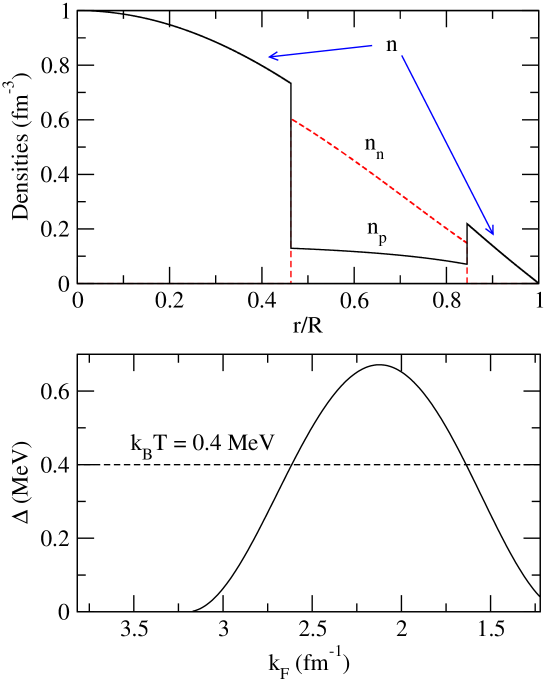
The superfluid energy gap varies with the density, cf. Fig. 1, and for any given temperature one would expect the transition to superfluidity to take place when . In a region of “strong superfluidity”, where , one can safely ignore finite temperature effects. However, as one approaches the phase transition (at points where ) excitations will play an increasing role. In fact, they dictate how the two distinct fluid degrees of freedom couple as one transits into the single-fluid regime. This transition problem has not yet been investigated in detail. Hence, we must make simplifications in order to proceed.
One can think of two natural limits. In the first, the particle reactions that drive the system towards chemical equilibrium are slow compared to the mode oscillation in the transition region, leading to a situation where a “superfluid” fluid element can temporarily move into the single fluid region without losing its identity. In that case, would be freely specificable at the interface. In the opposite limit, when reactions are faster than the timescale of oscillation, a fluid element that moves across the interface would immediately lose its identity. This would lock the velocities at the interface, and as a result would be linked to the single-fluid velocity . In our numerical calculations we assume that it is this latter scenario that applies. This is in contrast with Andersson et al. (2002), where it was assumed that reactions are slow.
III Analytic expansion for the local matter content
The perturbation equations require as input information about the bulk, multi-constituent, and entrainment effects. This necessarily leads to a number of coefficients to be determined. Admittedly, for those not familiar with the multi-fluid formalism (some of) these coefficients may seem somewhat obscure. In particular, since most of them tend to be ignored in discussions of the supranuclear equation of state. However, for our present purposes, the study of neutron star quasinormal modes, we can simplify the problem. To do this we consider an expansion of the master function that accounts for the fact that our background configuration is static and spherically symmetric. Alternatively, the expansion can be interpreted as one where the fluid velocities are small compared to the speed of light Andersson et al. (2002); Comer and Joynt (2003). For mode oscillations, this is a reasonable assumption. It is also expected to be accurate for slow-rotation models, see Andersson and Comer (2001).
Consider, for example, a term like . In principle, it implies that we need to expand the master function to . On the scale of a fluid element spacetime can be taken to be that of Minkowski. The term can then be written as
| (82) |
where and are, respectively, the neutron and proton three-velocities in the local Minkowski frame. When the individual three-velocities satisfy , then up to first-order in the ratio .
With this as our guide we write the master function in the form Andersson et al. (2002); Comer and Joynt (2003)
| (83) |
The bulk, multi-constituent, and entrainment coefficients thus become
| (84) | |||||
| (86) | |||||
| (88) | |||||
| (90) | |||||
| (92) | |||||
| (94) |
The and coefficients on the background are
| (95) |
This implies for the background chemical potentials that
| (96) |
In the single-fluid case, is the energy density, and so the chemical potential above is equal to that of the single-fluid result. We now see that the other coefficients simplify to
| (97) |
To gain a little further insight, a local, plane wave analysis Andersson and Comer (2007) indicates that the sound speeds (plural, because there are two) are the solutions to
| (98) |
We see that in addition to the expected bulk contribution to the sound speed (through and ) we have also entrainment entering via and the “symmetry energy” through . These effects at the local level have global consequences. For example, Andersson et al Andersson et al. (2002) have shown that entrainment has an impact on the oscillation mode spectrum by introducing so-called “avoided crossings” between the ordinary and superfluid modes as the entrainment is varied. Prix et al Prix et al. (2002) have demonstrated that the symmetry energy leaves its imprint on slowly rotating configurations when the neutrons and protons are not co-rotating.
Another dramatic effect of the entrainment is that it may facilitate a two-stream instability Andersson et al. (2003, 2004). In principle, such instabilities may operate in any system with two inter-penetrating components moving at different speeds. The key requirement for the instability to act is that the the two fluids are coupled, and entrainment can facilitate this coupling. The superfluid two-stream instability is being considered as a possible trigger for glitches and appears to be consistent with seven years of glitch data from the fastest known young pulsar J0537 Middleditch et al. (2006).
IV Equation of State Input
IV.1 Master Function Modulo Entrainment
In our numerical calculations we will compare two relatively simple parametrisations for the equation of state. Nothing prevents us from considering other perhaps more realistic models, including tabulated equation of state data, but at this point we are more concerned with the technical developments than with the actual numerical results. As we will discuss below, see Sec. VI, a fully consistent model requires information that is not yet available. Until this changes, this kind of analysis must be viewed as somewhat qualitative.
We consider two models for : i) a simple “TOY” model that is a sum of polytropes for the neutrons and protons, a symmetry energy term, and a final term that accounts for a relativistic gas of electrons, and ii) the more realistic, so-called “PAL” equation of state Prakash et al. (1988).
Specifically, the TOY model in the one-fluid and two-fluid layers takes the form
| (99) |
where we have chosen the parameters , , , , , is the baryon mass, and is the proton fraction. As shown in Table 1, this combination leads to a neutron star model with reasonable mass and radius.
The particular PAL master function for both layers is Andersson et al. (2004)
| (100) |
where
| (101) | |||||
| (103) | |||||
| (105) | |||||
| (107) | |||||
| (109) |
with (), , , , , , , , , , and . Again, the values for mass and radius obtained for these parameter values are reasonable, see Table 1.
| Model | ||||
|---|---|---|---|---|
| TOY | — | 1.0 | 1.635 | 10.655 |
| 0.45 | 1.0 | 1.745 | 10.641 | |
| PAL | 0.5 | 1.0 | 1.751 | 10.661 |
| 0.55 | 1.0 | 1.759 | 10.684 |
The electron contribution is vital for ensuring chemical equilibrium of the system. Even though the electron mass is much smaller than the nucleon mass (), the fact that the electrons are ultra-relativistic gives them enough energy to affect the chemical potential at the same level as the nucleons. Because of overall charge neutrality we set , and recall that the electrons and the protons flow together. Note also that, even though the imposition of chemical equilibrium will effectively make the single-fluid and two-fluid equations of state the same on the background, we have to distinguish them because of the , , etc. coefficients, for which the partial derivatives must be computed before chemical equilibrium is imposed.
IV.2 Gap Model
BCS theory is the basic paradigm for Fermionic superfluidity. Given a many-particle system with an attractive component in the interactions, the theory tells us that Cooper pairs will form, leading to a fundamental modification of the energy states near the Fermi surface, namely the formation of a gap in the energy spectrum. It is the existence of this gap that leads to superfluidity and in the present context multi-fluid dynamics. Even if particles try to scatter dissipatively, there are essentially no accessible states for them to scatter into unless there is enough energy to break a Cooper pair. When pair-breaking occurs the particles can reach the states above the gap, and energy can be irreversibly dissipated. Those particles in energy states “below” the Fermi surface are in this sense also “superfluid” since they cannot enter already filled states. So, for example, when neutrons are superfluid, ordinary scattering that would cause (on average) neutrons and protons to flow as a single fluid is severely diminished. It is thus clear that neutron star dynamics on a macroscopic scale is dictated by the gap structure on the microscopic scale.
There has been much work analyzing the details of the gap structure in dense, nucleonic matter trying to account for different interactions, medium effects etcetera (see Lombardo and Schulze (2001) for a review of gaps in general and Andersson et al. (2005) for an application to neutron stars). If even our rudimentary understanding of the strong force is correct for the densities expected in neutron stars there is little doubt that neutron and proton gaps exist. But given the complexities of the problem there is no exact agreement on the details; particularly on the density dependence of the gap. This affects the maximum gap energy, the gap profile as a function of density, and the size of regions in which gaps exist. However, it is generally accepted that neutron superfluidity and proton superconductivity will not extend throughout the star. Consequently, there should be layers having ordinary, single-fluid dynamics as well as ones where the multi-fluid description applies. This implies that most, if not all, previous mode calculations and modeling of rotational equilibria that assume superfluidity throughout the star are incomplete (see Comer (2002); Andersson and Comer (2007) for reviews).
As a first step towards improving the situation we will consider models that account for the detailed energy gap and its dependence on, in particular, the density. For practical reasons, we will use the parametrized model of Kaminker et al. (2001); Yakovlev et al. (2001); Kaminker et al. (2002); Yakovlev et al. (2002) as adapted by Andersson et al Andersson et al. (2005). This model has a number of “free” parameters, that can be used, for instance, to adjust the maximum gap energy and the gap profile (as a function of density). In this phenomenological description, the gap energy (where is the wave-number at the Fermi surface) takes the form
| (110) |
Note that density dependence enters implicitly through the wave-number . Andersson et al Andersson et al. (2005) provide a table of parameter values representative of the various gap calculations in the extant literature. For our numerical calculations we focus on gap model “h” given in their Table 1.
Once an equilibrium configuration is built, and density is known as a function of radius, we can use the gap energy to determine which layers of the equilibrium configuration are ordinary or superfluid. This requires an assumption of the temperature profile in the star. In principle, our calculations assume that the fluid is at zero temperature, somewhat in the same spirit as mode-damping calculations due to shear and/or bulk viscosity Andersson (2003). We certainly do not have a consistent temperature description. However, for our present purposes, this is not a major problem. The gap information that we use is phenomenological so it should be acceptable to account for the temperature in an approximate way as well. In view of this, we simply assume that the fluid is isothermal (and do not account for the gravitational redshift).
It would certainly be possible to improve on this description and it will eventually be important to do so. However, one would then like to account for all temperature effects, including quasiparticle excitations in the superfluid. This is an interesting problem since it opens the door for studies of dissipative superfluid neutron stars, but we will not discuss it further here.
Once we have chosen a core temperature we can work out if there are superfluid regions in the star. Varying the temperature thus affects the size of the superfluid layer, but has only a small effect on global parameters like the mass and radius, see Table 1. We also adapt the number of independent fluids for the mode calculations accordingly. For our canonical TOY and PAL neutron star models, the particle number density and gap energy as a function of radius typically take the form shown in Fig. 1. As anticipated, there is a layering of regions having different fluid dynamics. Wherever the gap energy is greater than the thermal energy , the neutrons will be superfluid, and therefore two-fluid dynamics will apply.
IV.3 The - Relativistic Mean Field Model
The model to be used for entrainment has been obtained using a relativistic mean field model of the type described by Glendenning Glendenning (1997). Whatever reservations one may have about mean-field equations of state, the great advantage from our present perspective is that the entrainment can be quantified. The Lagrangian for this system is given by
| (111) |
where
| (112) | |||||
| (114) | |||||
| (116) | |||||
| (118) |
Here is the baryon mass, is an 8-component spinor with the proton components as the top 4 and the neutron components as the bottom 4, the are the corresponding block diagonal Dirac matrices, and . The coupled set of field equations obtained from this Lagrangian are to be solved in each fluid element.
The main approximations of the mean field approach are to assume that the nucleons can be represented as plane-wave states and that all gradients of the and fields can be ignored. The coupling constants and and field masses and are determined, for instance, from properties of nuclear matter at the nuclear saturation density. Fortunately, in what follows, we only need to provide the ratios and .
The main aim here is to produce a master function that incorporates the entrainment effect. Consider again fluid elements somewhere in the neutron star. The fermionic nature of the nucleons means that they are to be placed into the various energy levels (obtained from the mean field calculation) until their respective (local) Fermi spheres are filled. The Fermi spheres are surfaces in momentum space. The entrainment is incorporated by displacing the center of the proton Fermi sphere from that of the neutron Fermi sphere. The neutron sphere is centered on the origin, and has a radius . Displaced an amount from the origin is the center of the proton sphere, which has a radius . The Fermi sphere radii and displacement are functions of the local neutron and proton number densities and the local, relative velocity of the protons, say, with respect to the neutrons.
Earlier we discussed the analytic expansion that applies to the master function, and determined that we need to know the and coefficients. The mean field model yields Comer and Joynt (2003)
| (121) | |||||
where the Dirac effective mass is the solution to the transcendental equation
| (124) | |||||
and each nucleon number density is related to its Fermi surface radius via
| (125) |
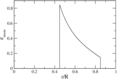
Typical behaviour of the entrainment parameter used in several studies, defined as
| (126) |
is shown in Fig. 2. We set and in what follows. These values are consistent with known nuclear matter properties and generate reasonable neutron star models Glendenning (1997); Comer and Joynt (2003).
V Numerical Results
We consider three variations on the mode calculations: i) changing the master function, ii) including (or not) entrainment, and iii) varying the temperature. As we have already discussed, the main effect of the latter is to alter the size of the two-fluid layer. Since the parameter space is vast, and we are mainly interested in understanding the qualitative effects, we restrict our discussion to a few “canonical” background models. These determine the total mass and radius given a particular central baryon number density , obtained by first specifying and then finding through the condition of chemical equilibrium. Of course, as we vary the temperature of the star, the matter distribution is affected which, in principle, changes the values of and . However, we find that these changes are negligible for the TOY model, and only slight for the PAL model (cf. Table 1 and the disscusion in Sec. IV.2).
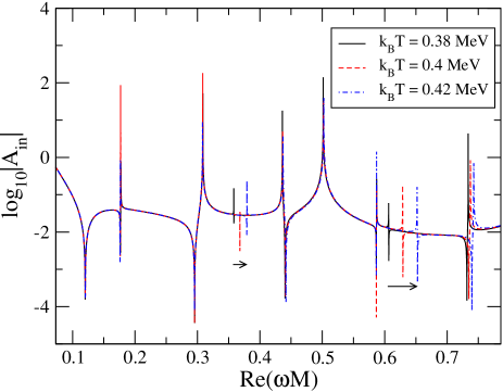
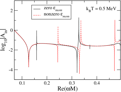
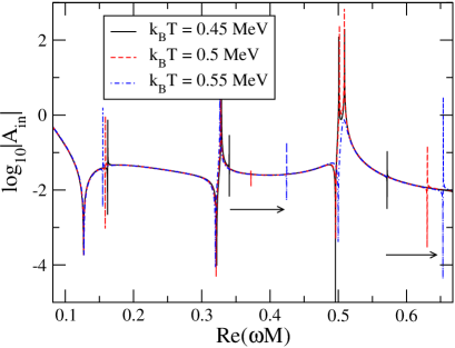
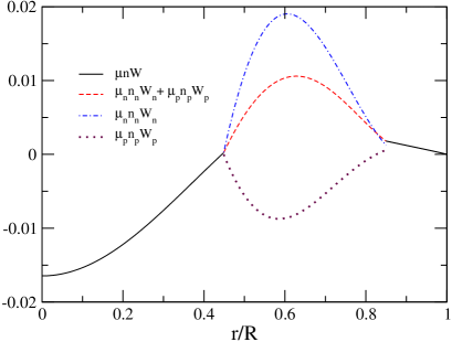
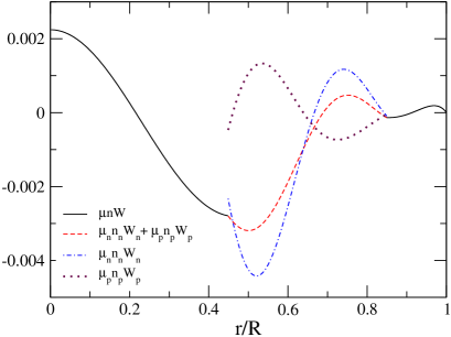
A quasinormal mode corresponds to a purely outgoing (gravitational) wave solution to the perturbation equations. The asymptotic amplitude for ingoing waves, , can therefore be used to locate the modes. Figs. 3, 4, 5, and 6 show this amplitude versus frequency for different models (see Comer et al. (1999) for the definition of ). The real part of the different quasinormal-mode frequencies can be approximated by the values that make vanish (or tend to ). This technique does not provide the damping times of the modes due to gravitational-wave emission. In practice, we can use the technique described by Andersson et al Andersson et al. (2002) to reliably determine the damping times. Our present discussion will, however, focus on the oscillation frequencies. Figs. 7, 8, and 9 provide the radial profiles of mode eigenfunctions for the first few frequencies.
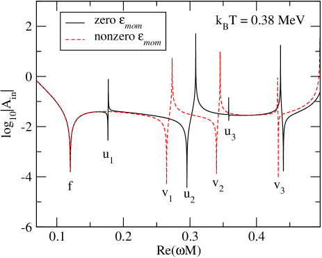
Several features of the mode spectrum are important to note. As in previous studies Comer et al. (1999); Andersson et al. (2002) of the general relativistic two-fluid system, there are “more modes” than in the single-fluid case. This is expected since we have an additional fluid degree of freedom (albeit localised to a distinct layer in the star). From Fig. 3 we see that entrainment has a small effect on the first mode in the spectrum, the f-mode, but clearly affects the next, a “superfluid” mode, frequency by shifting it from the value labelled to that labelled . Such behaviour is consonant with the local analysis of Andersson and Comer Andersson and Comer (2001), who show that the additional, superfluid modes depend on entrainment, while the fundamental f-mode does not.
From Fig. 4 we see that as the size of the two-fluid layer is decreased most of the mode frequencies remain largely unchanged. However, in this model there are clear “gap” modes (emphasised by the arrows) whose defining characteristic is that the layer thickness (i.e. the size of the gap energy relative to the temperature ) has significant impact on the frequency. As might be expected the frequencies increase as the thickness decreases. This is natural since the mode wavelengths must adjust to the size of the “container”.
For a semi-realistic determination of mode frequencies we consider Figs. 5 and 6 which show vs for the PAL master function. Qualitatively, Fig. 5 shows that the effect of entrainment in the PAL model is the same as for the TOY model. Perhaps more interesting is the observation that the layer thickness affects all modes in the PAL model, cf. Fig. 6. However, the most pronounced change is that the second “gap” mode (indicated by the arrow on the right of the figure) occurs earlier in the mode spectrum than in the case of the TOY model. Hence it seems clear that the combined background master function and the gap data are to some extent distinguishable via the mode spectrum.
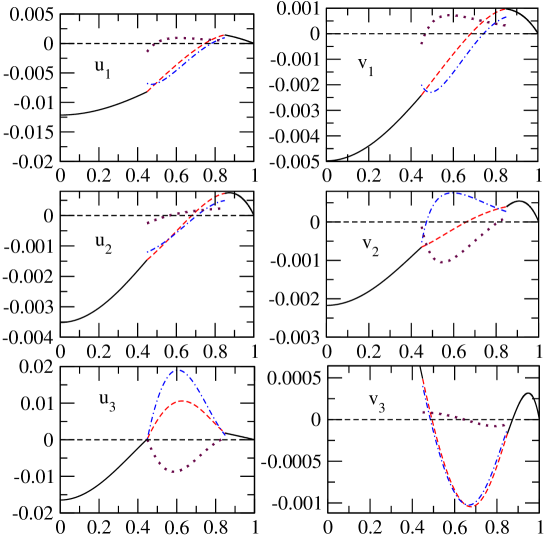
As expected, the radial mode profiles have a richer structure than in the single-fluid case. There are also marked differences with models where the two fluids extend throughout the core Comer et al. (1999); Andersson et al. (2002). In each of Figs. 7, 8, and 9, the solid line represents the total baryon flow in the one-fluid regions. In each two-fluid region the dot-dashed line represents the neutron flow, the dotted line represents the proton flow, and the dashed line represents the net baryon flow. Note that the boundary conditions between the one- and two-fluid regions imply that the net baryon flow must be continuous.
In Figs. 7 and 8 we see a characteristic feature of superfluid modes, the counter-motion between the neutrons and protons. The final Fig. 9 illustrates the effect of entrainment. In the plot for the mode we see the beginnings of an “avoided” crossing. As first demonstrated by Andersson et al Andersson et al. (2002), when viewed as a function of the entrainment two neighbouring mode frequencies sometimes come close to crossing but veer off before intersection happens. Past this avoided crossing the two modes exchange character in the sense that a co-moving mode becomes counter-moving and vice versa.
VI Discussion: Next Generation Equations of State
In this work we have extended the general relativistic two-fluid formalism used to model quasinormal-mode oscillations in such a way that superfluid neutron gap data can be incorporated. The main point is that the presence of a gap not only increases the number of fluid degrees of freedom locally; it also introduces a dynamical layering in the sense that the number of fluid degrees of freedom can change depending on whether the thermal energy of the star in a region is greater or less than the gap energy. It is clear that this structure will also be important for stellar rotational equilibria (eg. as determined by a slow-rotation approximation).
In our models we analyzed the effects of different master functions, entrainment (obtained from a relativistic mean field model), symmetry energy, and the presence of a gap. We found that the effect of entrainment on the mode spectrum is qualitatively consistent with earlier studies. On the other hand, the combined effects of the gap and the master function have distinguishable effects on the mode spectrum. Basically, our results illustrate that any “realistic” model for oscillating superfluid neutron stars must account not only for the “bulk” equation of state, one must also incorporate the entrainment and the superfluid gap data in a consistent way. We have, of course, not done this. At this point our models are more or less phenomenological. However, we have demonstrated that the computational technology required for this kind of study is now in place. What is missing is the input microphysics.
At the present time there is, as far as we are aware, no single equation of state calculation that provides all the required parameters. This needs to change in the future. Furthermore, one must not forget the neutron star crust, where the lattice of nuclei will have elastic properties. These also need to be determined consistently.
Let us discuss what (in our view) is required from the next generation equations of state if we want to model mode oscillations of multi-fluid neutron stars. To some extent these demands should be relatively straightforward to meet. Like most complex models, realistic equations of state are presented in tabular form. The question is what to include in the table. For traditional reasons, the information usually given is the pressure as a function of density and/or temperature. This would be adequate if one were only interested in solving for a background configuration single-fluid star. The information is, however, not even complete for the oscillations of such models. In order to model the so-called g-modes, which are sensitive to both temperature and composition gradients, one would need also the various particle fractions. Moreover, the multi-fluid formalism presented here requires a number of additional quantities.
In our experience, the two-fluid problem is most simply understood as having two independent thermodynamic parameters, the two number densitites . We see from the background and perturbation equations in Section II that we require the set of values . Each variable is a function of , and hence they will need to be given as two-dimensional arrays, the first index of each array standing for , say, and the second for . Of course, one usually assumes chemical equilibrium among the particle species on the background, which implies, say, that . However, a number of the quantities that are needed for the perturbation analysis, like the entrainment , require information about the system away from equilibrium. If we let represent the set of thermodynamic variables, then a sample tabular equation of state could look something like that of Table 2.
| … | ||||
| … | ||||
|
|
|
|
|
|
| … |
Can this information be provided within a single framework for determining the “equation of state”? We do not see why it should not be possible. Some of the quantities we require are already calculated, they are simply not presented in the final equation of state table. It should certainly be very easy to include the particle fraction in the tabulated data, and we see no reason why the entrainment coefficients should not be straightforward to determine as well. It is obviously the case that there is no universally agreed upon equation of state, or indeed method for its determination. From our point of view this is less relevant. We expect to live with uncertainties. After all, we do not have the luxury of having neutron stars readily available in the laboratory. The key point is that consistent models require all parameters to be consistent with a given microphysics calculation. Hopefully, an improved dialogue between neighbouring areas of research will allow us to make progress.
There are, of course, a number of related challenges. We have not yet satisfactorily answered the question of the minimal number of independent fluid degrees of freedom required to model a compact star. Glitch data tells us already that there are at least two. But what if we think about the deep core, quark deconfinement and CFL matter Alford (2004); Alford et al. (2000)? Do the various Cooper pairings between quarks indicate the presence of independent “fluids”? If they do, then what physical mechanisms exist to excite the additional degrees of freedom, and what is their physical interpretation? How can one hope to calculate the myriad of phases that could occur and then translate that into numerical models of rotating and oscillating multi-fluid compact stars? These are challenging questions that require further consideration.
Acknowledgements.
LML is supported in part by the Hong Kong Research Grants Council (grant numbers 401905 and 401807) and a postdoctoral fellow scheme at the Chinese University of Hong Kong. LML is also grateful for the hospitality of the Laboratoire de l’Univers et de ses Théories, Observatoire de Paris-Meudon where part of this work was done. NA gratefully acknowledges support from PPARC/STFC via grant numbers PP/E001025/1 and PP/C505791/1. GLC acknowledges partial support from NSF grant PHY-0457072.Appendix: Boundary conditions and numerical scheme
We have three different regions inside the star: (1) one-fluid core; (2) two-fluid superfluid region; and (3) one-fluid envelope. In the one-fluid regions, is the baryon number density (with being the chemical potential). In the superfluid region, and are the neutron and proton densities respectively (). Note that, in this Appendix, we use tildes to make a distinction between the variables in the single-fluid and the multi-flud regime. and denote the core-superfluid and superfluid-crust interfaces, respectively. We let denote the star’s radius.
The one-fluid regions are governed by 4 ODEs for
| (127) |
The superfluid region is governed by 6 ODEs for
| (128) |
VI.1 Boundary conditions
At , we have two conditions relating (cf Eqs. (A5)-(A6) of Comer et al Comer et al. (1999), with , , , etc. in our current notation). Explicitly, we have
| (129) |
and
| (130) |
At each of the interfaces ( and ), we have the following 4 junction conditions according to (A16)-(A18) of Andersson et al Andersson et al. (2002):
| (131) | |||||
| (132) | |||||
| (133) | |||||
| (134) |
where we have assumed that and are continuous across the interfaces.
We further impose that the two fluids move in lock-step at the interfaces. This effectively translates to the condition
| (135) |
In summary, Eqs. (131)-(135) are the required boundary conditions at the interfaces.
Finally, at the surface of the star , we have the single condition
| (136) |
VI.2 Numerical scheme
At , we need only to specify . The remaining variables are determined by Eqs. (129)-(130). All of the second derivatives , , etc. are also determined. We choose two arbitrary values of and integrate the 4 ODEs from small up to the core-superfluid interface . The general solution in the core region is
| (137) |
Next we turn to the general solution in the superfluid region . At , the solution must satisfy the condition (135). This means that we must generate 5 linearly independent solutions. This is obtained by choosing five different sets of (with ) and integrating to . The general solution in this domain is
| (138) |
At the surface, our solution must satisfy . Hence, we must generate 3 linearly independent solutions in the crust (). The general solution in this domain is
| (139) |
After fixing the overall normalization by choosing the value of one of the (says, ), we have 9 remaining constants () to be determined by the boundary conditions at and .
References
- Andersson and Comer (2007) N. Andersson and G. L. Comer, Living Reviews in Relativity 10, 1 (2007).
- Andersson and Comer (2006) N. Andersson and G. L. Comer, Class. Quant. Grav. 23, 5505 (2006).
- Lorimer (2005) D. R. Lorimer, Living Reviews in Relativity 8, 7 (2005).
- Lombardo (1999) U. Lombardo, in Nuclear Methods and the Nuclear Equation of State, edited by M. Baldo (World Scientific, Singapore, 1999), p. 458.
- Lombardo and Schulze (2001) U. Lombardo and H.-J. Schulze, LNP Vol. 578: Physics of Neutron Star Interiors 578, 30 (2001).
- Andersson et al. (2005) N. Andersson, G. L. Comer, and K. Glampedakis, Nucl. Phys. A 763, 212 (2005).
- Radhakrishnan and Manchester (1969) V. Radhakrishnan and R. N. Manchester, Nature (London) 244, 228 (1969).
- Lyne (1993) A. G. Lyne, in Pulsars as Physics Laboratories, edited by R. D. Blandford, A. Hewish, A. G. Lyne, and L. Mestel (Oxford University Press, Oxford, 1993), pp. 29–38.
- Migdal (1959) A. B. Migdal, Nucl. Phys. 13, 655 (1959).
- Clark et al. (1992) J. W. Clark, R. D. Dave, and J. M. C. Chen, in Structure and Evolution of Neutron Stars, edited by D. Pines, R. Tamagaki, and S. Tsuruta (Addison-Wesley Publishing Company, Redwood, CA, 1992), p. 134.
- Glendenning (1997) N. Glendenning, Nuclear and particle physics of compact stars (Springer, Berlin, Germany, 1997).
- Walecka (1995) J. D. Walecka, Oxford Stud. Nucl. Phys. 16, 1 (1995).
- Pethick and Ravenhall (1995) C. J. Pethick and D. G. Ravenhall, Annual Review of Nuclear and Particle Science 45, 429 (1995).
- Hoffberg et al. (1970) M. Hoffberg, A. E. Glassgold, R. W. Richardson, and M. Ruderman, Phys. Rev. Lett. 24, 775 (1970).
- Alford (2004) M. Alford, Progress of Theoretical Physics Supplement 153, 1 (2004).
- Alford et al. (2000) M. Alford, J. Berger, and K. Rajagopal, Nucl. Phys. B 571, 269 (2000).
- Gusakov (2007) M. E. Gusakov (2007), eprint arXiv:0704.1071 [astro-ph].
- Andersson et al. (2002) N. Andersson, G. L. Comer, and D. Langlois, Phys. Rev. D 66, 104002 (2002).
- Samuelsson and Andersson (2007) L. Samuelsson and N. Andersson, Mon. Not. R. Astro. Soc. 374, 256 (2007).
- Carter and Samuelsson (2006) B. Carter and L. Samuelsson, Class. Quant. Grav. 23, 5367 (2006).
- Andreev and Bashkin (1975) A. F. Andreev and E. P. Bashkin, Sov. Phys. JETP 42, 164 (1975).
- Vardanyan and Sedrakyan (1981) G. A. Vardanyan and D. M. Sedrakyan, Sov. Phys. JETP 54, 919 (1981).
- Alpar et al. (1984) M. A. Alpar, S. A. Langer, and J. A. Sauls, Ap. J. 282, 533 (1984).
- Comer and Joynt (2003) G. L. Comer and R. Joynt, Phys. Rev. D 68, 023002 (2003).
- Carter (1989) B. Carter, in Relativistic Fluid Dynamics (Noto, 1987), edited by A. Anile and M. Choquet-Bruhat (Springer-Verlag, Heidelberg, Germany, 1989), vol. 1385 of Lecture Notes in Mathematics, pp. 1–64.
- Comer and Langlois (1993) G. L. Comer and D. Langlois, Class. Quant. Grav. 10, 2317 (1993).
- Comer and Langlois (1994) G. L. Comer and D. Langlois, Class. Quant. Grav. 11, 709 (1994).
- Carter and Langlois (1995) B. Carter and D. Langlois, Nucl. Phys. B 454, 402 (1995).
- Langlois et al. (1998) D. Langlois, D. M. Sedrakian, and B. Carter, Mon. Not. R. Astro. Soc. 297, 1189 (1998).
- Comer et al. (1999) G. L. Comer, D. Langlois, and L. M. Lin, Phys. Rev. D 60, 104025 (1999).
- Prix (2000) R. Prix, Phys. Rev. D 62, 103005 (2000).
- Andersson and Comer (2001) N. Andersson and G. L. Comer, Class. Quant. Grav. 18, 969 (2001).
- Comer (2002) G. L. Comer, Found. Phys. 32, 1903 (2002).
- Prix (2004) R. Prix, Phys. Rev. D 69, 043001 (2004).
- Prix et al. (2002) R. Prix, G. L. Comer, and N. Andersson, Astron. Astrophys. 381, 178 (2002).
- Regge and Wheeler (1957) T. Regge and J. A. Wheeler, Phys. Rev. 108, 1063 (1957).
- Lindblom and Detweiler (1983) L. Lindblom and S. L. Detweiler, Ap. J., Suppl. Ser. 53, 73 (1983).
- Detweiler and Lindblom (1985) S. Detweiler and L. Lindblom, Ap. J. 292, 12 (1985).
- Andersson et al. (2003) N. Andersson, G. L. Comer, and R. Prix, Phys. Rev. Lett. 90, 091101 (2003).
- Andersson et al. (2004) N. Andersson, G. L. Comer, and R. Prix, Mon. Not. R. Astro. Soc. 354, 101 (2004).
- Middleditch et al. (2006) J. Middleditch, F. E. Marshall, Q. D. Wang, E. V. Gotthelf, and W. Zhang, Ap. J. 652, 1531 (2006).
- Prakash et al. (1988) M. Prakash, T. L. Ainsworth, and J. M. Lattimer, Phys. Rev. Lett. 61, 2518 (1988).
- Kaminker et al. (2001) A. D. Kaminker, P. Haensel, and D. G. Yakovlev, Astron. Astrophys. 373, L17 (2001).
- Yakovlev et al. (2001) D. G. Yakovlev, A. D. Kaminker, and O. Y. Gnedin, Astron. Astrophys. 379, L5 (2001).
- Kaminker et al. (2002) A. D. Kaminker, D. G. Yakovlev, and O. Y. Gnedin, Astron. Astrophys. 383, 1076 (2002).
- Yakovlev et al. (2002) D. G. Yakovlev, O. Y. Gnedin, A. D. Kaminker, and A. Y. Potekhin, in Neutron Stars, Pulsars, and Supernova Remnants, edited by W. Becker, H. Lesch, and J. Trümper (2002), p. 287.
- Andersson (2003) N. Andersson, Class. Quant. Grav. 20, 105 (2003).
- Andersson and Comer (2001) N. Andersson and G. Comer, Mon. Not. R. Astro. Soc. 328, 1129 (2001).