Determination of $F_{\pi}$ from Distributions of Dirac Operator Eigenvalues with Imaginary Density

Abstract:

In the $\epsilon$-regime of lattice QCD one can get an accurate measurement of the pion decay constant $F_{\pi}$ by monitoring how just one single Dirac operator eigenvalue splits into two when subjected to two different external vector sources. Because we choose imaginary chemical potentials our Dirac eigenvalues remain real. Based on the relevant chiral Random Two-Matrix Theory we derive individual eigenvalue distributions in terms of density correlations functions to leading order in the finite-volume $\epsilon$-expansion. As a simple byproduct we also show how the associated individual Dirac eigenvalue distributions and their correlations can be computed directly from the effective chiral Lagrangian.

1 Introduction

The distribution of individual Dirac operator eigenvalues have become a popular tool since their calculation [1] in the chiral Random Matrix Theory that is equivalent to the leading-order expression for the QCD partition function in the $\epsilon$-regime [2]. The analytical expressions distinguish very clearly between different gauge theories and different sectors of topology, as first shown in [3]. This has by now been verified by many different groups using different versions of fermions with different levels of chiral symmetry on the lattice. It has also become clear how to derive the same expression in the $\epsilon$-regime of chiral perturbations theory ($\epsilon\chi$PT) [4].

Individual eigenvalue distributions provide perhaps the most efficient tool to extract one of the low energy constants (LEC) in $\chi$PT, the infinite-volume chiral condensate $\Sigma$. Here we extend this analysis to the second LEC in line, the pion decay constant $F_{\pi}$, exploiting the fact that a nonvanishing chemical potential $\mu$ couples to $F_{\pi}$ to leading order in the $\epsilon$-expansion [5]. This method has been first suggested for imaginary isospin chemical potential with two different sets of Dirac eigenvalues [6]. The advantage over real $\mu$ [7] is that the Dirac operator retains its anti-hermiticity, allowing for unquenched simulations without encountering any sign-problems, and with greatly reduced computer efforts associated with the computation of the lowest eigenvalues. The proposal [6] was based on the 2-point spectral correlation function computed from $\epsilon\chi$PT and verified their prediction on quenched and unquenched Lattice data. This was generalised in [8] where all spectral correlations where computed analytically from the shown equivalence with a corresponding chiral Random two-Matrix Theory (chR2MT) with $\mu_{1,2}$. The advantage here is that partial quenching is possible, by setting one of the $\mu_{j}$ to zero. Hence existing configurations with $\mu=0$ can be used to measure $F_{\pi}$. This idea was most recently applied to unquenched chiral fermions in [9]. Here we present first results for individual Dirac eigenvalue distributions.

In section 2 we introduce the chR2MT and its corresponding $\epsilon\chi$PT. Section 3 presents our results in a general setting, which is then illustrated pictorially in the simplest case, the quenched isospin densities in section 4. Section 5 gives our conclusions and comments on other results.

2 RMT and $\chi$PT with imaginary chemical potential

We start by defining the chR2MT for imaginary chemical potentials introduced and solved in [8]

$${\cal Z}_{chR2MT} \sim \int d\Phi d\Psi~{}\exp\left[-{N}{\rm Tr}\left(\Phi^{\dagger}\Phi+\Psi^{\dagger}\Psi\right)\right]\prod_{f=1}^{N_{f}}\det[{\cal D}(\mu_{f})+m_{f}]\ .$$ (1)

The anti-hermitian Dirac matrix ${\cal D}$ is given in terms of two complex, rectangular random matrices $\Phi$ and $\Psi$ of size $N\times(N+\nu)$ with Gaussian measure:

$${\mathcal{D}}(\mu_{f})=\left(\begin{array}[]{cc}0&i\Phi+i\mu_{f}\Psi\\ i\Phi^{\dagger}+i\mu_{f}\Psi^{\dagger}&0\end{array}\right)~{}.$$ (4)

Here $\nu$ corresponds to fixed gauge field topology in the usual way. In the following we restrict ourselves to the case of only two different chemical potentials, ${\mathcal{D}}(\mu_{1,2})\equiv{\mathcal{D}}_{1,2}$, with $N_{1,2}$ flavours each. Referring to ref. [8] for details, we can write down the corresponding eigenvalue representation:

$${\cal Z}_{chR2MT} = \int_{0}^{\infty}\prod_{i}^{N}\left(dx_{i}dy_{i}(x_{i}y_{i})^{\nu+1}\prod_{f1=1}^{N_{1}}(x_{i}^{2}+m_{f1}^{2})\prod_{f2=1}^{N_{2}}(y_{i}^{2}+m_{f2}^{2})\right)$$ (6)

$$\times\ \Delta_{N}(\{x^{2}\})\Delta_{N}(\{y^{2}\})\det\left[I_{\nu}(2dNx_{i}y_{j})\right]e^{-N\sum_{i}c_{1}x_{i}^{2}+c_{2}y_{i}^{2}},$$

where $x_{i}$ and $y_{i}$ are real positive eigenvalues of the matrices $\Phi+\mu_{1,2}\Psi$, respectively. The constants $c_{1,2}$ and $d$ depend on $\mu_{1,2}$ (see [8]). For later convenience we abbreviate the integrand or joint probability distribution function (jpdf) by ${\cal P}(\{x\},\{y\})$.

If we take the large-$N$ limit and identify $Nx_{i}\to V\Sigma x_{i}\equiv\hat{x}$, $Nm_{f1}\to V\Sigma m_{f1}\equiv\hat{m}_{f1}$, $2N\mu^{2}_{1}\to VF_{\pi}^{2}\mu^{2}_{1}\equiv\hat{\mu}_{1}^{2}$, and similarly for the second set $N_{2}$, the partition function eq. (6) becomes identical to the corresponding $\epsilon\chi$PT partition function [8]

$${\cal Z}_{\chi PT}={\int dU(N_{f})\det[U]^{\nu}}\exp\left[{{\mbox{Tr}}\frac{1}{4}{\mu^{2}F_{\pi}^{2}V}{[U,B][U^{\dagger},B]}+\frac{1}{2}V\Sigma{M_{f}}({U}+{U^{\dagger}})}\right]\ .$$ (7)

$F_{\pi}$ and $\Sigma$ have as source terms chemical potential through the charge matrix $B=$diag$(\mu_{1}\mbox{\bf 1}_{N_{1}},\mu_{2}\mbox{\bf 1}_{N_{2}})$, and the diagonal mass matrix $M_{f}=$diag$(\{m_{f1}\},\{m_{f2}\})$, respectively. For explicit results for these partition functions we refer to [8].

3 Results for individual Dirac eigenvalue distributions

In the following we first define all density correlations, all individual eigenvalues correlations (or gap probabilities), and then express the latter in terms of the former. This inversion relation is valid for any theory expressed in terms of Dirac eigenvalues, having a jpdf ${\cal P}(\{x\},\{y\})$ that is symmetric under exchange of all $x_{i}$ and all $y_{i}$ eigenvalues separately. This applies to our chR2MT eq. (6), its equivalent $\epsilon\chi$PT, or a Lattice QCD partition functions in terms of Dirac eigenvalues.

All density correlation functions are defined by integrating all but $k(l)$ eigenvalues of ${\cal D}_{1}({\cal D}_{2})$

$$R_{k,l}(x_{1},\ldots,x_{k},\ y_{1},\ldots,y_{l}) \equiv \frac{N!^{2}}{(N-k)!(N-l)!{\cal Z}}\int_{0}^{\infty}\prod_{i=k+1}^{N}dx_{i}\prod_{j=l+1}^{N}dy_{j}{\cal P}(\{x\},\{y\})\ .$$ (8)

The simplest nontrivial example is the probability density $R_{1,1}(x,y)$ for finding an eigenvalue of ${\cal D}_{1}$ at $x$ and of ${\cal D}_{2}$ at $y$. If all eigenvalues of one kind are integrated out one finds back the known quantities of the one-matrix theory at $\mu=0$ [8]. Next we define the following gap probabilities that the interval $[0,s]$ is occupied by $k$ eigenvalues and $[s,\infty)$ by $(N-k)$ eigenvalues of ${\cal D}_{1}$, and that the interval $[0,t]$ is occupied by $l$ eigenvalues and $[t,\infty)$ by $(N-l)$ eigenvalues of ${\cal D}_{2}$:

$$E_{k,l}(s,t) \equiv \frac{N!^{2}}{(N-k)!(N-l!){\cal Z}}\int_{0}^{s}dx_{1}\ldots dx_{k}\int_{s}^{\infty}dx_{k+1}\ldots dx_{N}\int_{0}^{t}dx_{1}\ldots dx_{l}\int_{t}^{\infty}dy_{l+1}\ldots dy_{N}$$ (9)

$$\times\ {\cal P}(\{x\},\{y\})\ ,\ \ \mbox{for}\ k,l=0,1,\ldots,N\ \ .$$

The simplest example is $E_{0,0}(s,t)$ to find the intervals $[0,s]$ and $[0,t]$ empty of ${\cal D}_{1}$- and ${\cal D}_{2}$-eigenvalues, respectively. Similarly we can define the probability to find the $k$-th ${\cal D}_{1}$-eigenvalue at value $x_{k}=s$, and the $l$-th ${\cal D}_{2}$-eigenvalue at value $y_{l}=t$, to be

$$p_{k,l}(s,t) \equiv k{N\choose k}l{N\choose l}\frac{1}{{\cal Z}}\int_{0}^{s}dx_{1}\ldots dx_{k-1}\int_{s}^{\infty}dx_{k+1}\ldots dx_{N}\int_{0}^{t}dy_{1}\ldots dy_{l-1}\int_{t}^{\infty}dy_{l+1}\ldots dy_{N}$$ (10)

$$\times\ {\cal P}(x_{1},\ldots,x_{k-1},x_{k}=s,x_{k+1},\ldots,x_{N},y_{1},\ldots,y_{l-1},y_{l}=t,x_{l+1},\ldots,y_{N})\ ,$$

where the eigenvalues are ordered $x_{1}\leq\ldots\leq x_{N}$ and $y_{1}\leq\ldots\leq y_{N}$. The simplest example is $p_{1,1}(s,t)$, the distribution of each first eigenvalue. It is easy to see [10] that all the quantities eq. (10) can be obtained from eq. (9) by taking two derivatives,

$$\frac{\partial^{2}}{\partial s\partial_{t}}E_{k,l}(s,t)\ =\ k!\ l!\left(p_{k,l}(s,t)-p_{k+1,l}(s,t)-p_{k+1,l}(s,t)+p_{k+1,l+1}(s,t)\right)\ .$$ (11)

Here, we define $p_{k,l}=0$ whenever index $k$ or $l$ is zero. Finally we give an inversion formula expressing all gap probabilities, and hence all individual eigenvalue distributions in terms of densities:

$$E_{k,l}(s,t)=\sum_{i=0}^{N-k}\sum_{j=0}^{N-l}\frac{(-)^{i+j}}{i!j!}\int_{0}^{s}dx_{1}\ldots dx_{k+i}\int_{0}^{t}dy_{1}\ldots dy_{l+j}R_{(k+i,l+j)}(x_{1},\ldots,x_{k+i},\ y_{1},\ldots,y_{l+j}).$$ (12)

The derivation [10] follows closely the $\mu=0$ case [4]. Since it is known how to generate all higher density correlations $R_{k,l}$ from resolvents by inserting additional, auxiliary pairs of fermions and bosons e.g. into eq. (7), this relation clarifies how to generate individual eigenvalue distributions in this setting from field theory.

4 Examples

We discuss in detail the simplest example, the probability $p_{1,1}(s,t)$. It follows from the gap probability using eq. (11):

$$\frac{\partial^{2}}{\partial s\partial t}E_{0,0}(s,t)\ =\ p_{1,1}(s,t)\ .$$ (13)

We expand $E_{0,0}(s,t)$ to include at most 3-point density correlations as an approximation,

$$E_{0,0}(s,t) = 1-\int_{0}^{s}dx\,R_{1,0}(x)-\int_{0}^{t}dy\,R_{0,1}(y)+\int_{0}^{s}dx\int_{0}^{t}dyR_{1,1}(x,y)$$ (14)

$$+\frac{1}{2}\int_{0}^{t}dy_{1}dy_{2}\,R_{0,2}(y_{1},y_{2})+\frac{1}{2}\int_{0}^{s}dx_{1}dx_{2}\,R_{2,0}(x_{1},x_{2})$$

$$-\frac{1}{2}\int_{0}^{s}dx_{1}dx_{2}\int_{0}^{t}dy\,R_{2,1}(x_{1},x_{2},y)-\frac{1}{2}\int_{0}^{s}dx\int_{0}^{t}dy_{1}dy_{2}\,R_{1,2}(x,y_{1},y_{2})\ +\ \ldots$$

The derivatives eliminate all integrals over one-matrix densities that only depend on $s$ or $t$:

$$p_{1,1}(s,t)\ =\ R_{1,1}(s,t)\ -\ \int_{0}^{s}dx\,R_{2,1}(x,s,t)\ -\ \int_{0}^{t}dy\,R_{1,2}(s,t,y)\ +\ \ldots\ .$$ (15)

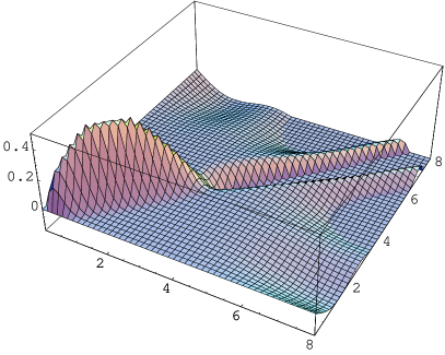
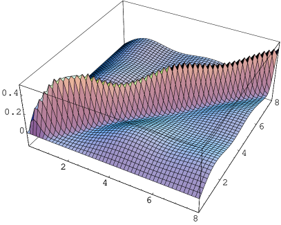
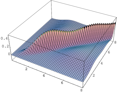
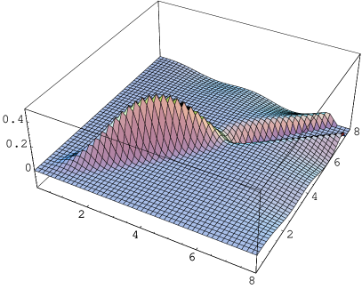
The leading order term is obviously given by the density $R_{1,1}(s,t)$, as can be clearly seen in figs. 1 and 3.

Figure 1: Example quenched density $R_{1,1}(s,t)$ (top left) vs individual eigenvalue distribution $p_{1,1}(s,t)$ (top right) at $\nu=0$ and $2\hat{\mu}=0.159$. The lower plots show corresponding 2D cuts at fixed $s=2$.

There, we display the quenched density in the case of imaginary isospin chemical potential $\mu_{1}=-\mu_{2}\equiv-\mu$. In the microscopic large-$N$ limit $\rho_{1,1}(\hat{x},\hat{y})=\lim_{N\to\infty}R_{1,1}(x=\hat{x}/N,y=\hat{y}/N)$ we obtain the following result [6, 8]

$$\rho_{(1,1)}(\hat{x},\hat{y}) = \rho_{(1,0)}(\hat{x})\rho_{(0,1)}(\hat{y})-\hat{x}\hat{y}{\cal K}^{+}(\hat{y},\hat{x})\left({\cal K}^{-}(\hat{x},\hat{y})-\frac{1}{4\hat{\mu}^{2}}I_{\nu}\left(\frac{\hat{x}\hat{y}}{4\hat{\mu}^{2}}\right)e^{-\frac{\hat{x}^{2}+\hat{y}^{2}}{8\hat{\mu}^{2}}}\right)$$

$${\cal K}^{\pm}(\hat{x},\hat{y}) \equiv \int_{0}^{1}dtt\,e^{\pm 2\hat{\mu}^{2}t^{2}}J_{\nu}(\hat{x}t)J_{\nu}(\hat{y}t)\ ,\ \ {\cal K}^{0}(\hat{x},\hat{y})\equiv\int_{0}^{1}dtt\,J_{\nu}(\hat{x}t)J_{\nu}(\hat{y}t)\ .$$ (16)

Here also the well known one-matrix density appears,

$$\rho_{(1,0)}(\hat{x})=\rho_{(0,1)}(\hat{x})=\frac{\hat{x}}{2}\left[J_{\nu}^{2}(\hat{x})-J_{\nu+1}(\hat{x})J_{\nu-1}(\hat{x})\right]\ =\ {\cal K}^{0}(\hat{x},\hat{x})~{},$$ (17)

see fig. 2. Eq. (16) was derived independently for the chR2MT eq. (6) [8] and prior to that for $\epsilon\chi$PT eq. (7) using replicas and the Toda-lattice hierarchy [6]. It is displayed in figs. 1 and 3 left for topological charge $\nu=0$ and 1, respectively, including 2-dimensional cuts. Because the density is the expectation value $R_{1,1}(x,y)\sim\left\langle\ {\mbox{Tr}}\delta({\cal D}_{1}-x)\ {\mbox{Tr}}\delta({\cal D}_{2}-y)\ \right\rangle$, $\mu\neq 0$ resolves the delta function $\delta(x-y)$ that we would obtain at $\mu=0$, times the one-matrix density eq. (17) that we give for comparison.

Figure 2: The one-matrix density $\rho_{(1,0)}(\hat{x})$ vs. the exact distribution of the first eigenvalue for $\nu=0$ : $p_{1}(\hat{x})=\frac{1}{2}\hat{x}\ e^{-\frac{1}{4}\hat{x}^{2}}$ (left), and for $\nu=1$ : $p_{1}(\hat{x})=\frac{1}{2}\hat{x}\ e^{-\frac{1}{4}\hat{x}^{2}}I_{2}(\hat{x})$ (right).

Next we move to individual eigenvalues. A closed determinantal expression for all higher density correlation functions in terms of the same building blocks as in eq. (16) was given in [8]:

$$\rho_{k,l}(\{{\hat{x}}\},\{{\hat{y}}\})=\prod_{i}^{k}x_{i}\prod_{j}^{l}y_{j}\det\!\left[\begin{array}[]{cc}{\mathcal{K}}^{0}(\hat{x}_{i_{1}},\hat{x}_{i_{2}})&\ \ {\mathcal{K}}^{-}(\hat{x}_{i_{1}},\hat{y}_{j_{2}})-\frac{1}{4\hat{\mu}^{2}}I_{\nu}\left(\frac{\hat{x}_{i_{1}}\hat{y}_{j_{2}}}{4\hat{\mu}^{2}}\right)e^{-\frac{\hat{x}_{i_{1}}^{2}+\hat{y}_{j_{2}}^{2}}{8\hat{\mu}^{2}}}\\ {\mathcal{K}}^{+}(\hat{y}_{j_{1}},\hat{x}_{i_{2}})&{\mathcal{K}}^{0}(\hat{y}_{j_{1}},\hat{x}_{j_{2}})\end{array}\right].$$ (18)

We can insert these formulas into the expansion eq. (15), after taking the microscopic limit. The result truncated at the given order is plotted in figs. 1 and 3 right. The fact that the truncated sum is an approximation is seen from the fact that the individual eigenvalue density becomes negative (or diverges when adding higher order terms). For the given values in the figs. this happens above $s=t\approx 4$, and we have cut the 3D plots at values below $-0.15$. Higher order terms in the expansion eq. (12) will keep the individual eigenvalue distribution to be zero for larger values of $s$ and $t$. From our experience with the case $\mu=0$ [4] we expect that this expansion converges fast. The next to leading order used in the figures gives already a reasonably good approximation.

Figure 3: Same as fig. 1. for $\nu=1$. The exact zero eigenvalues push the density away from the origin.

5 Conclusions and outlook

We have shown how to derive individual eigenvalues distributions $p_{k,l}$ for two sets of real Dirac operators with different imaginary chemical potentials $\mu_{1,2}$. Similar expressions have been derived for a single Dirac operator with complex eigenvalues at real $\mu$ and compared to Lattice data [11]. Both types of $\mu$ couple to $F_{\pi}$ and thus allow to fully determine all LECs in the leading order $\chi$PT Lagrangian. But only imaginary $\mu$ with real Dirac eigenvalues allow to date to perform unquenched or partially quenched simulations. The equivalence of $\epsilon\chi$PT to the chR2MT we mentioned here for the density and partition function has been derived very recently for all correlators [12].

We have given an effective expansion for the distributions $p_{kl}$ by truncating the sum over integrated densities, as was illustrated in our examples. The possibility to derive exact expressions (which is possible for real $\mu$) is currently under investigation [10]. Our hope is that the results presented here will become as useful as previously for $\mu=0$.

References

• [1] S. M. Nishigaki, P. H. Damgaard and T. Wettig, Phys. Rev. D58 (1998) 087704 [hep-th/9803007]; P. H. Damgaard and S. M. Nishigaki, Phys. Rev. D63 (2001) 045012 [hep-th/0006111].
• [2] E. V. Shuryak and J. J. M. Verbaarschot, Nucl. Phys. A560 (1993) 306 [hep-th/9212088].
• [3] R.G. Edwards , Urs M. Heller, Joe Kiskis and Rajamani Narayanan, Phys. Rev. Lett. 82 (1999) 4188. [hep-th/9902117].
• [4] G. Akemann and P. H. Damgaard, Phys. Lett. B583 (2004) 199 [hep-th/0311171].
• [5] D. Toublan and J.J.M. Verbaarschot, Nucl. Phys. B603 (2001) 343 [hep-th/0012144].
• [6] P. H. Damgaard, U. M. Heller, K. Splittorff and B. Svetitsky, Phys. Rev.  D 72 (2005) 091501 [hep-lat/0508029]; P. H. Damgaard, U. M. Heller, K. Splittorff, B. Svetitsky and D. Toublan, Phys. Rev.  D 73 (2006) 074023 [hep-lat/0602030]; Phys. Rev.  D 73 (2006) 105016 [hep-th/0604054].
• [7] G. Akemann and T. Wettig, Phys. Rev. Lett. 92 (2004) 102002 Erratum-ibid. 96 (2006) 029902 [hep-lat/0308003]; J. C. Osborn and T. Wettig, PoS (LAT2005) 200 [hep-lat/0510115].
• [8] G. Akemann, P. H. Damgaard, J. C. Osborn and K. Splittorff, Nucl. Phys. B [hep-th/0609059].
• [9] T. DeGrand, S. Schaefer, arXiv:0708.1731v1 (see also in these proceedings).
• [10] G. Akemann and P. H. Damgaard, unpublished, 2007
• [11] G. Akemann, J. Bloch L. Shifrin and T. Wettig, PoS(Lattice2007)224, these proceedings.
• [12] F. Basile, G. Akemann, unpublished, 2007