Abstract

We consider solutions of (super) gravities associated to non-critical (super) string theories in arbitrary space-time dimension $D=p+3$, that describe generically non extremal black $p$-branes charged under NSNS or RR gauge fields, embedded in some non critical vacuum. In the case of vacuum (uncharged) backgrounds, we solve completely the problem obtaining all the possible solutions, that consist of the $(p+1)$-dimensional Minkowski space times a linear dilaton times a $S^{1}$, and a three parameter family of solutions that include $(p+1)$-dimensional Minkowski space times the cigar, and its T-dual $(p+1)$-dimensional Minkowski space times the trumpet. For NSNS charged solutions, we also solve in closed form the problem, obtaining several families of solutions, that include in particular the fundamental non-critical string solution embedded in the cigar vacuum, recently found in hep-th/0604202, a solution that we interpret as a fundamental non-critical string embedded in the linear dilaton vacuum, and a two-parameter family of regular curvature solutions asymptotic to $AdS_{1,2}\times S^{1}$. In the case of RR charged $Dp$-branes solutions, an ansätz allows us to find a non conformal, constant curvature, asymptotically $AdS_{1,p+1}$ space, T-dual to $AdS_{1,p+2}$, together with a two-parameter family of solutions that includes the non conformal, $AdS$ black hole like solution associated with the earlier space. The solutions obtained by T-duality are Einstein spaces consisting of a two-parameter family of conformal, constant dilaton solutions, that include, in particular, the AdS black hole of hep-th/0403254. We speculate about the possible applications of some of them in the framework of the gauge-gravity correspondence.

1 Introduction

The AdS/CFT correspondence and further generalizations [1] have turned to be an interesting way of addressing the old problem of solving the low energy dynamics of gauge theories, through the realization of the holographic ideas in the context of superstring theories in non trivial vacua. So far, the most interesting results were obtained mainly for supersymmetric (SUSY) field theories, in the supergravity (SUGRA) limit [2]. In reference [3], a possible mechanism to get holographic gravity duals of non supersymmetric gauge theories was proposed, by compactifying supersymmetric systems in higher dimensions with antiperiodic, SUSY breaking, boundary conditions for the fermions. However, the holographic set-up in all these cases suffers from several limitations, derived from the impossibility, at the present, to quantize strings on Ramond-Ramond (RR) backgrounds. Due to this fact, a low energy, SUGRA approximation becomes necessary. On the other hand, the existence of transverse, compact spaces, leads to Kaluza-Klein (KK) towers of states with masses of order of the gauge theory scale (and then, of the scale of hadronic states), that therefore do not decouple from the theory and contaminate the spectrum. The introduction of non critical backgrounds (in dimensions $D<10$) provides a natural way to overcome this problem. The idea to extend the holographic description of gauge theories to non critical backgrounds was first introduced by Alexander Polyakov [4], who proposed a dual of pure Yang-Mills (YM) theories in terms of a five dimensional non critical gravity background.

Non critical string theories in $D$ dimensional space-time are characterized by including on their world-sheet (at least) one scalar field, the Liouville mode, which combines together with additional $D-1$ coordinates [5], [6]. Much work was made on the subject in the past, in particular in $D\leq 2$ and the related matrix models [7]. However, the so called “$c=1$ barrier” seemed to forbid to go to higher dimensions [8]. Things change dramatically with the introduction of $({\cal N}_{L},{\cal N}_{R})=(2,2)$ superconformal symmetry on the world-sheet. In reference [9], it was showed that non critical type II superstring theories can be formulated in $d=2n,n=0,1,\dots,4$ space-time dimensions, and describe consistent solutions of string theory in sub-critical dimensions, with space-time supersymmetry consisting of, at least, $2^{n+1}$ supercharges. On the world-sheet, these theories present, in addition to the dynamical Liouville mode $\phi$ mentioned above, a compact boson $X$, being the target space of the general form

$${\cal M}^{d}\times\Re_{\phi}\times S^{1}\times M/\Gamma\qquad,$$ (1.1)

where ${\cal M}^{d}$ is $d$-dimensional Minkowski space-time, $M$ is an arbitrary $(2,2)$ superconformal field theory, and $\Gamma$ a discrete subgroup acting on $S^{1}\times M$. Now, the Liouville theory include a linear dilaton background that yields a strong coupling singularity; however the existence of the compact boson allow to resolve this singularity by replacing the $\Re_{\phi}\times S^{1}$ part of the background by the ${\cal N}=2$ Kazama-Suzuki supercoset $SL(2,\Re)_{k}/U(1)$. This space has a two-dimensional cigar-shaped geometry, with a natural scale given by $\sqrt{k\,\alpha^{\prime}}$ [10], [12]. It provides a geometric cut-off for the strong coupling singularity, while coinciding with the linear dilaton solution in the weak coupling region. It is known that this vacuum solution is an exact solution to all orders in type II theories, up to a trivial shift $k\rightarrow k-2$ [13]. When $d=8$, we go back to the critical superstring in flat ten dimensional Minkowski space-time.

In view of this, we will consider in this paper backgrounds of type II non critical string theories that include a two dimensional non trivial sector parameterized by a radial coordinate and a $S^{1}$ coordinate, the radial coordinate having the interpretation of a energy scale from the field theory point of view [4], [14], [15]. In reference [16] the solution of a fundamental non critical string placed at the tip of the cigar and localized also at the origin of the transverse space was presented. We will consider here general $p$-branes with different charges that fills all Minkowski space (no transverse space).

Some papers addressing similar problems have appeared in the literature, most notably reference [17] (see also [18], [19], [20]). But, rather than approach the problem through a set of BPS equations (hopefully supersymmetric) derived from a superpotential that relates to the potential of the system, we prefer to solve systematically the full system of second order equations of motion.

An important point to remark is the following one. The fact of being outside criticality leads, in some cases, to solutions trustable in a large region of the space, as it is the case of [16] and some solutions presented in this paper, much in the same way as it happens with the $p$-brane solutions of critical theories. In other cases, like in $AdS$ type solutions, the curvature in string units is of order unity, and it is not clear if they receive important corrections from the higher order terms in the effective action. We adopt, along the lines followed in [4], [18], [17], [21], [24], the posture that for special solutions like the $AdS$ like ones, the conformal structure of the background would not be modified by the higher order curvature contributions but only the corresponding parameters will get renormalized.

The paper is organized as follows. In Section $2$ we present the non-critical low energy effective action, and the equations of motion corresponding to the space-time filling $p$-brane ansätz to be considered, and reduce the full system of second order differential equations to a pair of coupled equations plus a constraint, “zero energy” condition, equations (2.36) and (2.39) respectively. In Section $3$ we obtain all the possible vacuum solutions. They consist of the solution given by Minkowski space-time times a linear dilaton times $S^{1}$, plus a three-parameter family asymptotic to it but singular in general, excluding a two-parameter sub-family (that includes the well-known Minkowski space-time times the cigar), regular in the sense that it presents bounded both the string coupling constant and the scalar curvature. In Section $4$ we solve completely the problem for NSNS charged solutions. Other than the well-known $AdS_{1,2}\times S^{1}$ space-time (represented by the exact $SL(2,\Re)\times U(1)$ model), there are several families of solutions which have it as an asymptotic limit. Most notably, a solution interpretable as a fundamental non critical string embedded in the linear dilaton vacuum, and a two-parameter family of regular solutions. Moreover we recover the solution of fundamental string in the cigar vacuum recently found, and we also get three families of oscillating, singular solutions, with no obvious interpretation. In Section $5$ we consider the system for RR charged solutions; under an assumption we are able to get a two-parameter family of solutions asymptotic to a space-time T-dual of $AdS_{1,p+2}$ space, singular in the infrared limit except two regular solutions. Nevertheless, via a T-duality transformation, it maps into a conformal, constant dilaton family of Einstein spaces that includes the $AdS$ black hole of [17]. In Section $6$ we draw the conclusions and future perspectives. An appendix that collects the formulae used in the computations is added at the end.

2 The general setting.

2.1 The non critical action and the space-time filling $p$-brane ansätz.

Our starting point is the bosonic part of the low energy effective action of non critical (super) strings in $D$ dimensions, that in string frame reads,

$$S[\Psi] = \frac{1}{2\,\kappa_{D}{}^{2}}\;\int\epsilon_{G}\;e^{-2\Phi}\left(R[G]+4\left(D\Phi\right)^{2}+\Lambda^{2}-{1\over 2}\sum_{q}e^{\left({b_{q}}+2\right)\Phi}\left(F_{q+2}\right)^{2}\right)\qquad.$$ (2.1)

Here $\Psi$ stands for the fields $\{G_{mn},\Phi,A_{q+1}\}$, $F_{q+2}=dA_{q+1}$ is the field strength of the gauge field form $A_{q+1}$, and $\epsilon_{G}=\omega^{0}\wedge\dots\wedge\omega^{D-1}=d^{D}x\,\sqrt{-\det G}\,$ is the volume element. The constant $b_{q}$ is equal to $-2(0)$ for NSNS (RR) forms, $\Lambda^{2}$ is a cosmological constant (assumed positive) that we identify in (super) string theories with ($\frac{10-D}{\alpha^{\prime}}$) $\frac{2\,(26-D)}{3\,\alpha^{\prime}}$, and $\kappa_{D}{}^{2}$ is the $D$-dimensional Newton constant. Furthermore, we assume a source term of the form,

$$S^{source}[\Psi]=\sum_{q}\;\mu_{q}\,\int A_{q+1}\wedge*J_{q+1}$$ (2.2)

where $\mu_{q}$ is the charge of the source under $A_{q+1}$. The equations of motion that follow are,

$$R_{mn} = -2\,D_{m}D_{n}\Phi+T^{A}_{mn}$$ (2.3)

$$\Lambda^{2} = e^{2\Phi}D^{2}(e^{-2\Phi})+\sum_{q}{D\,(2+b_{q})-2\,b_{q}-4(q+2)\over 8}\;e^{(2+b_{q})\Phi}\;(F_{q+2})^{2}$$ (2.4)

$$d\left(e^{b_{q}\,\Phi}*F_{q+2}\right) = (-)^{q}\;Q_{q}\;*J_{q+1}\;\;\;\;,\;\;\;\;Q_{q}\equiv 2\,\kappa_{D}{}^{2}\,\mu_{q}$$ (2.5)

where the gauge energy-momentum tensor and strength field contractions are ,

$$T^{A}_{mn} \equiv \sum_{q}{1\over 2}\,e^{(2+b_{q})\Phi}\left(\left(F_{q+2}\right)^{2}_{mn}-\frac{2+b_{q}}{4}\;G_{mn}\;\left(F_{q+2}\right)^{2}\right)$$ (2.6)

$$(F_{q+2})^{2}_{mn} \equiv \frac{1}{(q+1)!}\,G^{m_{1}n_{1}}\dots G^{m_{q+1}n_{q+1}}\;{F_{q+2}}_{mm_{1}\dots m_{q+1}}{F_{q+2}}_{nn_{1}\dots n_{q+1}}$$ (2.7)

$$(F_{q+2})^{2} \equiv \frac{1}{(q+2)!}G^{m_{1}n_{1}}\dots G^{m_{q+2}n_{q+2}}\;{F_{q+2}}_{m_{1}\dots m_{q+2}}{F_{q+2}}_{n_{1}\dots n_{q+2}}$$ (2.8)

Let us now consider the following ansätz for the fields,

$$G = -A^{2}\;dx^{0}{}^{2}+\tilde{A}^{2}\;d{\vec{x}}{}^{2}+C^{2}\;d\rho^{2}+\tilde{C}^{2}\;dz^{2}$$ (2.10)

$$A_{p+1} = dx^{0}\wedge\dots\wedge dx^{p}\;E(\rho)$$ (2.11)

$$\Phi = \Phi(\rho)$$ (2.12)

where we have assumed that there is one type of charge, corresponding to the $A_{p+1}$ form (only $q=p$ is present). This ansätz would correspond to a black $p$-brane extended along $(x^{0},\vec{x})$, and localized along the radial variable $\rho$ in the transverse two dimensional euclidean space with coordinates ($\rho,z$), preserving $SO(2)$ rotational invariance in the $S^{1}$ variable $z$, whose compactification radius $R$, $z\sim z+2\,\pi\,R$, is determined in most cases by the charges. The vacuum solution in which it is embedded, in view of the non zero cosmological constant $\Lambda$, must be non trivial (see Section $3$). In the appendix we collect relevant formulae related with this ansätz.

2.2 The equations of motion and the general solution.

When a p-brane fills all the Minkowski space, the transverse space is just two-dimensional and the solution, admitting a $SO(2)$ invariance, depends on the “radial” coordinate $\rho$ of the deformed space (linear dilaton, cigar, etc, see Section $3$). By realizing that $C(\rho)$ is defined up to a $\rho$-reparameterization (in fact, it transforms as a one form, all the other metric functions being scalar), it is natural to search for a scalar variable under such diffeomorphisms. This is accomplished by the introduction of the coordinate $x$, defined in the following way ,

$$x = \int^{\rho}\;\frac{d\rho}{H(\rho)}\;\;\;\;,\;\;\;\;\partial_{x}=H(\rho)\;\partial_{\rho}$$ (2.13)

$$H \equiv \frac{F_{1}\;e^{-2\Phi}}{C^{2}}=A\;\tilde{A}^{p}\;\tilde{C}\;e^{-2\Phi}\;C^{-1}$$ (2.14)

Let us notice that $H$ is a vector and $F_{1}$ another $1$-form, and $H\,C$ a scalar. Furthermore,

$$C(\rho)\;d\rho=H\;C\;dx$$ (2.15)

an useful relation to write down the metric. In terms of this coordinate, and denoting with a prime a $x$-derivative, the equations of motion (A.44)-(A.50) take the following form,

$$(\ln A)^{\prime\prime} = \frac{2-b_{p}}{8}\;{e^{(2+b_{p})\Phi}\over(A{\tilde{A}}^{p})^{2}}\;E^{\prime 2}$$ (2.16)

$$(\ln\tilde{A})^{\prime\prime} = \frac{2-b_{p}}{8}\;{e^{(2+b_{p})\Phi}\over(A{\tilde{A}}^{p})^{2}}\;E^{\prime 2}$$ (2.17)

$$(\ln\tilde{C})^{\prime\prime} = -\frac{2+b_{p}}{8}\;{e^{(2+b_{p})\Phi}\over(A{\tilde{A}}^{p})^{2}}\;E^{\prime 2}$$ (2.18)

$$(\ln e^{-2\Phi})^{\prime\prime} = \Lambda^{2}\;(H\;C)^{2}-\frac{2-b_{p}}{8}\,(p+1)\;{e^{(2+b_{p})\Phi}\over(A{\tilde{A}}^{p})^{2}}\;E^{\prime 2}$$ (2.19)

$$\left(\frac{e^{(2+b_{p})\Phi}}{(A{\tilde{A}}^{p})^{2}}\;E^{\prime}\right)^{\prime} = (-)^{p+1}\,Q_{p}\;\frac{(H\;C)^{2}}{A{\tilde{A}}^{p}}\;e^{2\Phi}\;\delta^{2}_{G^{\perp}}$$ (2.20)

$$-(\ln H\,C)^{\prime\prime}+(\ln H\,C)^{\prime 2} = (\ln A)^{\prime 2}+p\,(\ln\tilde{A})^{\prime 2}+(\ln\tilde{C})^{\prime 2}-\frac{2-b_{p}}{8}\;{e^{(2+b_{p})\Phi}\over(A{\tilde{A}}^{p})^{2}}\;E^{\prime 2}$$ (2.21)

We have written at the end the $C$-equation, that we will take as a constraint equation coming from the gauge fixing of the coordinate $\rho$, implicitly made through the introduction of the coordinate $x$.

Let us start to solve these equations. Outside the location of the source, equation (2.20) is solved by,

$$E^{\prime}=q\;\left(A\;\tilde{A}^{p}\right)^{2}\,e^{-(2+b_{p})\Phi}$$ (2.23)

where $q$ is related to $Q_{p}$ by the relation (obtained by integration of (2.5)),

$$q=\frac{Q_{p}}{V_{z}}\qquad,\qquad V_{z}=\int\,dz$$ (2.24)

The solution of (2.16) is,

$$A=e^{\alpha\,x}\;\tilde{A}$$ (2.25)

while that the solution of (2.18) is,

$$\tilde{C}=e^{\gamma\,x}\;\tilde{A}^{-\frac{2+b_{p}}{2-b_{p}}}$$ (2.26)

where $\alpha,\gamma,$ are arbitrary constants. We remain with two equations, (2.17) and (2.19), plus the constraint (2.21). Let us introduce the following functions ,

$$f_{1}(x) \equiv (HC)^{2}=\left(A\;\tilde{A}^{p}\;\tilde{C}\;e^{-2\Phi}\right)^{2}=\left(e^{(\alpha+\gamma)\,x}\;\tilde{A}^{p+1-\frac{2+b_{p}}{2-b_{p}}}\;e^{-2\Phi}\right)^{2}$$ (2.27)

$$V_{z}{}^{2}\;f_{2}(x) \equiv \left({H\,C\over\tilde{C}}\right)^{2}\;e^{(2-b_{p})\Phi}=\left(A\;\tilde{A}^{p}\right)^{2}\;e^{-(2+b_{p})\Phi}=\left(e^{\alpha\,x}\;\tilde{A}^{p+1}\right)^{2}\;e^{-(2+b_{p})\Phi}$$ (2.28)

In terms of them, the solution for the fields is given by,

$$G = \tilde{A}^{2}\;\left(-e^{2\alpha\,x}\;dx^{0}{}^{2}+d\vec{x}^{2}\right)+f_{1}(x)\;dx^{2}+e^{2\gamma\,x}\;\tilde{A}^{-2\frac{2+b_{p}}{2-b_{p}}}\;dz^{2}$$ (2.30)

$$e^{2\sigma\Phi} = e^{2\left(\frac{2+b_{p}}{2-b_{p}}\alpha+(p+1)\gamma\right)\,x}\;\frac{(V_{z}{}^{2}\;f_{2})^{p+1-\frac{2+b_{p}}{2-b_{p}}}}{f_{1}{}^{p+1}}$$ (2.31)

$$F_{p+2} = V_{z}\;Q_{p}\;f_{2}(x)\;dx\wedge dx^{0}\wedge\dots\wedge dx^{p}$$ (2.32)

where

$$\tilde{A}^{2\sigma} = V_{z}{}^{4}\;e^{(-(2-b_{p})\alpha+(2+b_{p})\gamma)\,x}\;\frac{f_{2}{}^{2}}{f_{1}{}^{\frac{2+b_{p}}{2}}}$$ (2.33)

$$\sigma \equiv \frac{1}{2}\left((2-b_{p})(p+1)+\frac{(2+b_{p})^{2}}{2-b_{p}}\right)$$ (2.34)

It is not difficult to see that the equations (2.17) and (2.19) can be recast in terms of $f_{1},f_{2}$ in the following form,

$$(\ln f_{1})^{\prime\prime} = 2\,\Lambda^{2}\;f_{1}-{2+b_{p}\over 4}\,Q_{p}{}^{2}\;f_{2}$$ (2.35)

$$(\ln f_{2})^{\prime\prime} = \frac{2+b_{p}}{2}\,\Lambda^{2}\;f_{1}+\frac{(2-b_{p})^{2}}{16}\,(p+1)\,Q_{p}^{2}\;f_{2}$$ (2.36)

while that the constraint (2.21) becomes,

$$-\frac{1}{2}\,(\ln f_{1})^{\prime\prime}+\frac{1}{4}\,(\ln f_{1})^{{}^{\prime}\>2} = \left((\ln\tilde{A})^{\prime}+\alpha\right)^{2}+p\,(\ln\tilde{A})^{\prime}{}^{2}+\left(-\frac{2+b_{p}}{2-b_{p}}\,(\ln\tilde{A})^{\prime}+\gamma\right)^{2}$$ (2.37)

$$- \frac{2-b_{p}}{8}\,Q_{p}{}^{2}\;f_{2}$$ (2.38)

$$2\,\sigma\,(\ln\tilde{A})^{\prime} = -(2-b_{p})\,\alpha+(2+b_{p})\,\gamma+\left(\ln\frac{f_{2}{}^{2}}{f_{1}{}^{\frac{2+b_{p}}{2}}}\right)^{\prime}\qquad.$$ (2.39)

In conclusion, the general solution (2.32) for space-time filling, non critical $p$-branes, is determined by the system (2.36) and the constraint (2.39).

Let us start a systematic survey of the possible solutions with the simplest case.

3 Uncharged solutions $Q_{p}=0$; the vacua.

The uncharged solutions represent the possible noncritical vacuum backgrounds. The system (2.36) reduces to,

$$(\ln f_{1})^{\prime\prime} = 2\,\Lambda^{2}\;f_{1}$$ (3.1)

$$(\ln f_{2})^{\prime\prime} = \frac{2+b_{p}}{2}\,\Lambda^{2}\;f_{1}$$ (3.2)

Plugging the first equation into the second one we obtain $f_{2}$ in terms of $f_{1}$,

$$f_{2}(x)=e^{\epsilon_{0}+\epsilon\,x}\;f_{1}(x)^{\frac{2+b_{p}}{4}}$$ (3.3)

where $\epsilon_{0},\epsilon$ are arbitrary constants. To solve for $f_{1}$, we rewrite the first equation in the form,

$$(\ln f_{1})^{\prime\prime}=2\,\Lambda^{2}\;f_{1}\;\;\longleftrightarrow\;\;{1\over f_{1}}{d\over dx}\left({1\over f_{1}}{d\over dx}f_{1}(x)\right)=2\,\Lambda^{2}\;\;\longleftrightarrow\;\;\frac{d^{2}f_{1}}{dy^{2}}=2\,\Lambda^{2}$$ (3.4)

where we have introduced the primitive $y(x)$ (relevant up to a constant),

$$y(x)=\int^{x}\;dx\;f_{1}(x)\;\;\longleftrightarrow\;\;f_{1}(x)=y^{\prime}(x)$$ (3.5)

By trivial integration in (3.4) we get,

$$f_{1}(x)=y^{\prime}(x)=\Lambda^{\>2}\;y(x)^{\>2}+2\,\beta\;y(x)+\gamma$$ (3.6)

where $\beta,\gamma$ are arbitrary integration constants, whose general solution is,

$$x-x_{0}=\int^{y(x)}{dy\over\Lambda^{\>2}\;y^{\>2}+2\,\beta\;y+\gamma}=\left\{\begin{array}[]{lcl}{1\over 2\,\sqrt{-\Delta}}\,\ln\left|{\Lambda^{2}y+\beta-\sqrt{-\Delta}\over\Lambda^{2}y+\beta+\sqrt{-\Delta}}\right|&,&\;\;\;\Delta<0\cr-{1\over\Lambda^{2}y+\beta}&,&\;\;\;\Delta=0\cr{1\over\sqrt{\Delta}}\,\arctan{\Lambda^{2}y+\beta\over\sqrt{\Delta}},&,&\;\;\;\Delta>0\end{array}\right.$$ (3.7)

where $\Delta=\Lambda^{2}\,\gamma-\beta^{2}$. Thus, we see there are three possible branches, depending of the sign of $\Delta$. The corresponding value of $y(x)$ is

$$\Lambda^{2}\,y(x)+\beta=\left\{\begin{array}[]{lcl}\begin{array}[]{lcl}-\sqrt{-\Delta}\>\coth\left(\sqrt{-\Delta}\,(x-x_{0})\right)&,&\;\;|\Lambda^{2}\,y(x)+\beta|>\sqrt{-\Delta}\cr-\sqrt{-\Delta}\>\tanh\left(\sqrt{-\Delta}\,(x-x_{0})\right)&,&\;\;|\Lambda^{2}\,y(x)+\beta|<\sqrt{-\Delta}\cr\end{array}&,&\Delta<0\cr-\frac{1}{x-x_{0}}&,&\Delta=0\cr\sqrt{\Delta}\,\tan\left(\sqrt{\Delta}\,(x-x_{0})\right)&,&\Delta>0\end{array}\right.$$ (3.8)

which yields, according to (3.6),

$$f_{1}(x)=\left\{\begin{array}[]{lcl}\begin{array}[]{lcl}-{\Delta\over\Lambda^{2}}\>{1\over\sinh^{2}\left(\sqrt{-\Delta}\,(x-x_{0})\right)}&,&\;\;|\Lambda^{2}\,y(x)+\beta|>\sqrt{-\Delta}\cr+{\Delta\over\Lambda^{2}}\>{1\over\cosh^{2}\left(\sqrt{-\Delta}\,(x-x_{0})\right)}&,&\;\;|\Lambda^{2}\,y(x)+\beta|<\sqrt{-\Delta}\cr\end{array}&,&\;\;\Delta<0\cr\frac{1}{\Lambda^{2}\,(x-x_{0})^{2}}&,&\;\;\Delta=0\cr{\Delta\over\Lambda^{2}}\>{1\over\cos^{2}\left(\sqrt{\Delta}\,(x-x_{0})\right)}&,&\;\;\Delta>0\qquad.\end{array}\right.$$ (3.9)

We see that $f_{1}$ depend on two free parameters, $x_{0}$ and $\Delta$, while that the whole solution (2.32) depends also non trivially (see below) on $\alpha,\epsilon,\gamma$. Let us pass to analyze each branch separately.

3.1 Solution with $\Delta=0$; the linear dilaton.

In this case, the constraint equation (2.39) enforces the condition $\alpha=\epsilon=\gamma=0$; from (3.9) we have,

$$f_{1} = {1\over\Lambda^{2}\,(x-x_{0})^{2}}$$ (3.10)

$$f_{2} = e^{\epsilon_{0}}\;\left({1\over\Lambda^{2}\,(x-x_{0})^{2}}\right)^{\frac{2+b_{p}}{4}}$$ (3.11)

By introducing the variable $Y=-\Lambda^{-1}\,\ln(\Lambda\,|x-x_{0}|)$, and after trivial re-scalings and redefinitions we get,

$$G = \eta_{1,p}+dY^{2}+r^{\prime}_{0}{}^{2}\;d\theta^{2}$$ (3.12)

$$\Phi = \Phi_{0}-\frac{1}{r_{0}}\,Y\qquad,\qquad r_{0}\equiv\frac{2}{\Lambda}$$ (3.13)

the direct product of $p+1$ dimensional Minkowski space-time and the linear dilaton solution times a $S^{1}$ (assuming $\theta\sim\theta+2\,\pi$) of arbitrary radius $r^{\prime}_{0}$. The linear dilaton is widely discussed in the literature, see [25], [26]. Furthermore, a Wick rotated version of this solution is considered as a cosmological model in [27].

3.2 Solutions with $\Delta<0$; the cigar and more.

From the definition (LABEL:f12def), $f_{1}=(H\,C)^{2}>0$, and therefore the physically relevant solution in (3.9) is the first one; then

$$f_{1}(x) = {-\Delta\over\Lambda^{2}}\>{1\over\sinh^{2}\left(\sqrt{-\Delta}\,(x-x_{0})\right)}$$ (3.14)

$$f_{2}(x) = e^{\epsilon_{0}+\epsilon\,x}\;\left({-\Delta\over\Lambda^{2}}\>{1\over\sinh^{2}\left(\sqrt{-\Delta}\,(x-x_{0})\right)}\right)^{\frac{2+b_{p}}{4}}$$ (3.15)

After various redefinitions we get the general solution in the form,

$$G = -e^{-2a\,x}\;dx^{0}{}^{2}+e^{-2e\,x}\;d\vec{x}{}^{2}+\frac{1}{\Lambda^{2}}\;\frac{dx^{2}}{\sinh^{2}x}+e^{-2g\,x}\;dz^{2}$$ (3.16)

$$e^{2\Phi} = 2\,e^{2\,\Phi_{0}}\;e^{-\varphi\,x}\;|\sinh x|\qquad,\qquad\varphi\equiv a+p\,e+g$$ (3.17)

while the constraint equation (2.39) reads,

$$a{}^{2}+p\,e{}^{2}+g{}^{2}=1$$ (3.18)

We can put the solution in a more familiar form by introducing the variables $\rho$ and $\theta$,

$$e^{-x}\equiv\tanh\rho\qquad,\qquad\theta\equiv\frac{\Lambda}{2}\,z$$ (3.19)

in terms of which, after trivial re-scalings of the $x^{\mu}$’s, the solution is written as,

$$G = -(\tanh\rho)^{2a}\;dx^{0}{}^{2}+(\tanh\rho)^{2e}\;d\vec{x}{}^{2}+{4\over\Lambda^{2}}\;\left(d\rho^{2}+(\tanh\rho)^{2g}\;d\theta^{2}\right)$$ (3.20)

$$e^{2\Phi} = e^{2\Phi_{0}}\>\>{(\sinh\rho)^{\varphi-1}\over(\cosh\rho)^{\varphi+1}}\qquad,\qquad\varphi\equiv a+p\,e+g$$ (3.21)

$$1 = a^{2}+p\,e^{2}+g^{2}$$ (3.22)

The solutions are determined, other than by $\Phi_{0}$, by the three parameters $a,e,g,$ subject to the constraint in the last equation of (3.22). All of them go asymptotically, i.e. for large $\rho$, to the linear dilaton of the past subsection. As particular solutions belonging to this three-parameter family, we have two well-known ones,

$a=e=0\;,g=1\>\>\>$

We get the vacuum solution corresponding to the direct product of $p+1$ dimensional Minkowski space and the cigar with scale $r_{0}=\frac{2}{\Lambda}$,

$$G = \eta_{1,p}+r_{0}^{2}\;\left(d^{2}\rho+\tanh^{2}\rho\;d\theta^{2}\right)$$ (3.23)

$$e^{2\Phi} = e^{2\Phi_{0}}\>\>{1\over\cosh^{2}\rho}$$ (3.24)

Here the periodicity $\theta\sim\theta+2\,\pi$ is imposed to avoid a conical singularity at the origin $\rho=0$.

$a=e=0\;,g=-1\>\>\>$

We get the vacuum solution corresponding to the direct product of $p+1$ dimensional Minkowski space and the trumpet,

$$G = \eta_{1,p}+r_{0}^{2}\;\left(d^{2}\rho+\coth^{2}\rho\;d\theta^{2}\right)$$ (3.25)

$$e^{2\Phi} = e^{2\Phi_{0}}\>\>{1\over\sinh^{2}\rho}$$ (3.26)

This solution is singular at the origin $\rho=0$. However it is well known that the cigar and the trumpet are related by T-duality. Both solutions correspond to exact two dimensional CFT on the world sheet, the gauged Wess-Zumino-Witten-Novikov (WZWN) model $SL(2,\Re)/U(1)$, with vector and axial gauging respectively [10], [11].

It is interesting to note that all the solutions present a non trivial dilaton; however for those with $\varphi\geq 1$ the string coupling $\,g_{s}\equiv e^{\Phi}\,$ is bounded everywhere, what assures us that perturbative string theory set-up is under control. But among them, there is a two-parameter family of solutions with special features, that which saturates the bound $\varphi=1$. In first term, they present the same dilaton of the cigar solution; it is also shown that this is the only case in which the parameter $\Phi_{0}$ is physical, in the sense that it is the value of the dilaton at some point (at the tip $\rho=0$). And what is more, from the Ricci scalar of these solutions,

$$R=\frac{\Lambda^{2}}{4}\;\frac{4\,\sinh^{2}\rho-(\varphi-1)^{2}+1-a^{2}-p\,e^{2}-g^{2}}{\sinh^{2}\rho\,\cosh^{2}\rho}=\frac{1}{r_{0}{}^{2}}\;\frac{4\,\sinh^{2}\rho-(\varphi-1)^{2}}{\sinh^{2}\rho\,\cosh^{2}\rho}$$ (3.27)

where in the last step we have made use of the constraint in (3.22), we see that they are the only regular solutions, their scalar curvature being the same as that of the cigar. Moreover, in contrast to the cigar solution, the other ones present necessarily a warp factor that diverges at $\rho=0$. For the two parameter $\varphi=1$ family, the Ricci tensor results,

$$R_{00}=-\frac{2\,a}{r_{0}{}^{2}}\;\frac{1}{\cosh^{2}\rho}\qquad \qquad R_{IJ}=\frac{2\,e}{r_{0}{}^{2}}\;\frac{1}{\cosh^{2}\rho}\;\delta_{IJ}$$ , (3.28)

$$R_{p+1p+1}=\frac{2}{r_{0}{}^{2}}\;\frac{1}{\cosh^{2}\rho}\qquad \qquad R_{p+2p+2}=\frac{2\,g}{r_{0}{}^{2}}\;\frac{1}{\cosh^{2}\rho}$$ , (3.29)

It would be interesting to see if some of the solutions (3.22) have an exact CFT field description as the cigar and trumpet do. We mention that in reference [30] the Einstein space corresponding to the solution $a=e=g=\frac{1}{\sqrt{p+2}}$ ($\varphi=\sqrt{p+2}$) was considered, while that the subfamily of possible vacua corresponding to $a=e$ appears recently in reference [17].

3.3 Solutions with $\Delta>0$.

The family of solutions is given by,

$$G = -e^{-2\,a\,x}\;dx^{0}{}^{2}+e^{-2\,e\,x}\;d\vec{x}{}^{2}+\frac{1}{\Lambda^{2}}\;\frac{dx^{2}}{\cos^{2}x}+e^{-2\,g\,x}\;dz^{2}$$ (3.30)

$$e^{2\Phi} = 2\,e^{2\,\Phi_{0}}\;e^{-\varphi\,x}\;|\cos x|\qquad,\qquad\varphi\equiv a+p\,e+g$$ (3.31)

However the constraint (3.18) is now replaced by,

$$a{}^{2}+p\,e{}^{2}+g{}^{2}=-1$$ (3.32)

We conclude that there exist no solutions in the branch $\Delta>0$.

We have exhausted all the possible uncharged solutions. Let us go to the case of charged solutions.

4 NSNS charged solutions, $Q_{p}\neq 0\;,\;b_{p}=-2$.

These solutions, from the string theory point of view, are relevant just for $p=1$, with the identification of the gauge field $A_{2}$ with the usual Kalb-Ramond two-form gauge field $B$, under which a fundamental string can be charged. We will maintain $p$ free however, fixing it in the analysis of relevant cases.

The equations for the $f_{i}$’s (2.36) get decoupled,

$$(\ln f_{1})^{\prime\prime} = 2\,\Lambda^{2}\;f_{1}$$ (4.1)

$$(\ln f_{2})^{\prime\prime} = (p+1)\,Q_{p}{}^{2}\;f_{2}$$ (4.2)

The solutions to each equation were worked out in the past section; we have from (3.9) and the positivity of $f_{i}$’s,

$$f_{1}(x)=\left\{\begin{array}[]{lcl}{-\Delta_{1}\over\Lambda^{2}}\>{1\over\sinh^{2}\left(\sqrt{-\Delta_{1}}\,(x-x_{1})\right)}&,&\;\;\Delta_{1}<0\cr\frac{1}{\Lambda^{2}\,(x-x_{1})^{2}}&,&\;\;\Delta_{1}=0\cr{\Delta_{1}\over\Lambda^{2}}\>{1\over\cos^{2}\left(\sqrt{\Delta_{1}}\,(x-x_{1})\right)}&,&\;\;\Delta_{1}>0\end{array}\right.$$ (4.3)

$$f_{2}(x)=\left\{\begin{array}[]{lcl}{-2\,\Delta_{2}\over(p+1)\,Q_{p}{}^{2}}\>{1\over\sinh^{2}\left(\sqrt{-\Delta_{2}}\,(x-x_{2})\right)}&,&\;\;\Delta_{2}<0\cr\frac{2}{(p+1)\,Q_{p}{}^{2}}\,\frac{1}{(x-x_{2})^{2}}&,&\;\;\Delta_{2}=0\cr{2\,\Delta_{2}\over(p+1)\,Q_{p}{}^{2}}\>{1\over\cos^{2}\left(\sqrt{\Delta_{2}}\,(x-x_{2})\right)}&,&\;\;\Delta_{2}>0\end{array}\right.$$ (4.4)

where $\Delta_{i},x_{i},$ are arbitrary constants. The fields are expressed as in (2.32),

$$G = e^{-\frac{2\alpha}{p+1}\,x}\;f_{2}{}^{\frac{1}{p+1}}\;\left(-e^{2\alpha\,x}\;dx^{0}{}^{2}+\;d\vec{x}{}^{2}\right)+f_{1}(x)\;dx^{2}+e^{2\gamma\,x}\;dz^{2}$$ (4.5)

$$e^{4\Phi} = V_{z}{}^{2}\,e^{2\gamma\,x}\;\frac{f_{2}}{f_{1}}$$ (4.6)

$$F_{p+2} = Q_{p}\,f_{2}(x)\;dx\wedge dx^{0}\wedge\dots\wedge dx^{p}$$ (4.7)

and then, they are determined by the choice of $f_{1}$ and $f_{2}$, and the imposition of the constraint (2.39), that reads,

$$\frac{\Delta_{2}}{p+1}-\Delta_{1}=\frac{p}{p+1}\;\alpha{}^{2}+\gamma{}^{2}$$ (4.8)

The solutions depend on the parameters $\alpha,\gamma,\Delta_{i},x_{i}$. We collect them below .

1. $\Delta_{1}=\Delta_{2}=0$

   $$G = |x-x_{0}|^{-\frac{2}{p+1}}\;\eta_{1,p}+\frac{1}{\Lambda^{2}}\;\frac{dx^{2}}{x^{2}}+R_{1}{}^{2}\;d\theta^{2}$$ (4.9)

   $$e^{2\,\Phi} = e^{2\,\Phi_{0}}\;\left|1-\frac{x_{0}}{x}\right|^{-1}$$ (4.10)

   $$F_{p+2} = s(q)\;\sqrt{\frac{2}{p+1}}\;\frac{1}{(x-x_{0})^{2}}\;dx\wedge dx^{0}\wedge\dots\wedge dx^{p}$$ (4.11)

   where $s(q)\equiv sign(q)$, and $\theta\sim\theta+2\,\pi$, being the $S^{1}$ radius fixed to be,

   $$R_{1}=\sqrt{\frac{p+1}{2}}\;\frac{|Q_{p}|\,e^{2\Phi_{0}}}{2\,\pi\,\Lambda}\qquad.$$ (4.12)

   According to the value of $x_{0}$, three possibilities are present.

   
   

   If $x_{0}=0$, with $x=(r_{0}\,u)^{-p-1}$ the solution reads,

   $$G = r_{0}{}^{2}\;\left(\frac{du^{2}}{u^{2}}+u^{2}\;\eta_{1,p}\right)+R_{1}{}^{2}\;d\theta^{2}\qquad,\qquad r_{0}\equiv\frac{p+1}{\Lambda}$$ (4.13)

   $$\Phi = \Phi_{0}$$ (4.14)

   $$F_{p+2} = -s(q)\sqrt{2\,(p+1)}\;r_{0}{}^{p+1}\;u^{p}\;du\wedge dx^{0}\wedge\dots\wedge dx^{p}$$ (4.15)

   
   

   It is a $AdS_{1,p+1}|_{r_{0}}\times S^{1}|_{R_{1}}$ space, with a constant dilaton. This background (for $p=1$) is well-known, it is the exact (super) CFT defined by the $Sl(2,\Re)_{-k}\times U(1)|_{R_{1}}$ WZWN model, with the level given by $(k)k-2=\frac{4}{\alpha^{\prime}\,\Lambda^{2}}$ [22].

   If $x_{0}<0$, after re-scaling $x^{\mu},x\rightarrow|x_{0}|^{\frac{1}{p+1}}\,x^{\mu}\,,|x_{0}|\,x$, and introducing the radial variable $r$,

   $$\frac{1}{1+x}=1-\left(\frac{r_{h}}{r}\right)^{p+1}=f(r),\qquad,\qquad r_{h}<r<\infty$$ (4.16)

   
   

   the solution takes the form,

   $$G = f(r)^{\frac{2}{p+1}}\;\eta_{1,p}+r_{0}{}^{2}\;\frac{dr^{2}}{r^{2}\,f(r)^{2}}+R_{1}{}^{2}\;d\theta^{2}$$ (4.17)

   $$e^{2\Phi} = e^{2\Phi_{0}}\;\left(\frac{r_{h}}{r}\right)^{p+1}$$ (4.18)

   $$F_{p+2} = s(q)\;\sqrt{2\,(p+1)}\;\frac{r_{h}{}^{p+1}}{r^{p+2}}\;\;dr\wedge dx^{0}\wedge\dots\wedge dx^{p}$$ (4.19)

   It is easy to see that this solution interpolates between the linear dilaton vacuum of Section $4.2$ (for large $r\gg r_{h}$) and the $AdS_{1,p+1}|_{r_{0}}\times S^{1}|_{R_{1}}$ space of (4.15) (for $r\rightarrow r_{h}{}^{+}$). We are tempted to identify it (for $p$=1) with a fundamental string ($F1$) embedded in the linear dilaton vacuum, the $AdS$ space being the near horizon limit that washes off the vacuum region, like usually happens in critical brane solutions . The scalar curvature is displayed in Figure $1$.

   

   Figure 1: The curve shows $\alpha^{\prime}\,R$ as a function of $\rho=r/r_{h}$, where $R$ is the scalar curvature corresponding to (4.19) and $1<\rho<\infty$.

   
   

   Finally, if $x_{0}>0$ we get,

   $$G = r_{0}{}^{2}\;\left(u^{2}\;\eta_{1,p}+\left(1+\left(r_{0}\,u\right)^{p+1}\right)^{-2}\;\frac{du^{2}}{u^{2}}\right)+R_{1}{}^{2}\;d\theta^{2}$$ (4.21)

   $$e^{2\Phi} = e^{2\Phi_{0}}\;\left(1+\left(r_{0}\,u\right)^{p+1}\right)$$ (4.22)

   $$F_{p+2} = -s(q)\;\sqrt{2\,(p+1)}\;r_{0}{}^{p+1}\;\;u^{p}\;du\wedge dx^{0}\wedge\dots\wedge dx^{p}$$ (4.23)

   which goes to $AdS_{1,p+1}|_{r_{0}}\times S^{1}|_{R_{1}}$ for $r_{0}\,u\rightarrow 0$, but it is singular in the large $u$ region $r_{0}\,u\rightarrow\infty$. The scalar curvature is displayed in Figure $2$.

   
   

   

   Figure 2: The curve shows $\alpha^{\prime}\,R$ as a function of $\rho=r_{0}\,u$, where $R$ is the scalar curvature corresponding to (4.23) and $0<\rho<\infty$.

2. $\Delta_{1}<0\;,\;\Delta_{2}=0$

   $$G = \frac{e^{-\frac{2\,a}{p+1}\,x}}{|x-x_{0}|^{\frac{2}{p+1}}}\;\left(-e^{2\,a\,x}\,dx^{0}{}^{2}+d{\bf x}^{2}\right)+\frac{1}{\Lambda^{2}}\,\frac{dx^{2}}{\sinh^{2}x}+R_{1}{}^{2}\,e^{2\,g\,x}\,d\theta^{2}$$ (4.24)

   $$e^{2\,\Phi} = e^{2\,\Phi_{0}}\,e^{g\,x}\;\left|\frac{\sinh x}{x-x_{0}}\right|$$ (4.25)

   $$F_{p+2} = s(q)\;\sqrt{\frac{2}{p+1}}\;\frac{1}{(x-x_{0})^{2}}\;dx\wedge dx^{0}\wedge\dots\wedge dx^{p}$$ (4.26)

   $$1 = \frac{p}{p+1}\,a^{2}+g^{2}$$ (4.27)

   where $R_{1}$ is given in (4.12). It is a two-parameter family of solutions, with three branches depending on the sign of $x_{0}$. Let us focus on the solutions with $a=0,g=-1$, that have a bounded string coupling at large $x$. A convenient change of variable is $e^{-x}=\tanh\rho$.

   If $x_{0}=0$, we get,

   $$G = |\ln\tanh\rho|^{-\frac{2}{p+1}}\;\eta_{1,p}+\frac{4}{\Lambda^{2}}\;d\rho^{2}+R_{1}{}^{2}\;\tanh^{2}\rho\;d\theta^{2}$$ (4.28)

   $$e^{-2\Phi} = 2\;e^{-2\Phi_{0}}\;\cosh^{2}\rho\;|\ln\tanh\rho|$$ (4.29)

   $$F_{p+2} = -s(q)\;\sqrt{\frac{2}{p+1}}\;\frac{1}{\sinh\rho\;\cosh\rho\;(\ln\tanh\rho)^{2}}\;d\rho\wedge dx^{0}\wedge\dots\wedge dx^{p}$$ (4.30)

   The solution results, for large $\rho$, asymptotic to the $AdS_{1,p+1}|_{\frac{p+1}{\Lambda}}\times S^{1}{}|_{R_{1}}$ solution of (4.15), but singular at $\rho=0$, where the world volume of the brane shrinks to zero size, and the $\Re^{2}$ transverse space presents a conical singularity, unless the relation $R_{1}=\frac{2}{\Lambda}$ (and therefore, $\,|Q_{p}|\,e^{2\Phi_{0}}\sim 1$) be imposed, in which case the transverse space is just the cigar. The scalar curvature is displayed in Figure $3$.

   

   Figure 3: The curve shows $\alpha^{\prime}\,R$ as a function of $\rho$, where $R$ is the scalar curvature corresponding to (LABEL:5.12), $r_{0}=2/\Lambda$, and $0<\rho<\infty$.

   If $x_{0}\neq 0$, after a re-scaling $x^{\mu}\rightarrow|x_{0}|^{\frac{1}{p+1}}\,x^{\mu}$, and the redefinition $e^{2\Phi_{0}}\rightarrow 2\,|x_{0}|\,e^{2\Phi_{0}}$, the solution reads,

   $$G = |U(\rho)|^{-\frac{2}{p+1}}\;\;\eta_{1,p}+\frac{4}{\Lambda^{2}}\,\left(d\rho^{2}+\tanh^{2}\rho\;d\theta^{2}\right)$$ (4.32)

   $$e^{-2\Phi} = e^{-2\Phi_{0}}\,\cosh^{2}\rho\;|U(\rho)|$$ (4.33)

   $$F_{p+2} = s(q\,x_{0})\;\sqrt{\frac{2}{p+1}}\;dU(\rho)^{-1}\wedge dx^{0}\wedge\dots\wedge dx^{p}$$ (4.34)

   where,

   $$U(\rho)=1+\frac{1}{x_{0}}\,\ln\tanh\rho\qquad,\qquad|x_{0}|\equiv\sqrt{\frac{2}{p+1}}\;\frac{2\pi}{|Q_{p}|}\,e^{-2\Phi_{0}}<0$$ (4.35)

   When $x_{0}<0$, we identify (for $p=1$) the solution as a fundamental non critical string embedded in the cigar vacuum. On the other hand, solutions with $x_{0}>0$ presents a singularity at $\rho=\rho_{0},\tanh\rho_{0}=e^{-\frac{2\pi}{|Q_{p}|e^{2\Phi_{0}}}}$. These solutions were recently discovered in reference [16]. The scalar curvature of them is displayed in Figure $4$.

   

   Figure 4: The curves show $\alpha^{\prime}\,R$ as a function of $\rho$ for different values of $x_{0}$, where $R$ is the scalar curvature corresponding to (4.34).

3. $\Delta_{1}<0\;,\;\Delta_{2}<0$

   $$G = \left(\frac{e^{-a\,x}}{|\sinh\left(k\,(x-x_{0})\right)|}\right)^{\frac{2}{p+1}}\left(-e^{2\,a\,x}dx^{0}{}^{2}+d\vec{x}{}^{2}\right)+\frac{1}{\Lambda^{2}}\,\frac{dx^{2}}{\sinh^{2}x}+R_{k}{}^{2}\,e^{2\,g\,x}\;d\theta^{2}$$ (4.36)

   $$e^{2\Phi} = e^{2\Phi_{0}}\,\frac{e^{g\,x}\;|\sinh x|}{|\sinh(k\,(x-x_{0}))|}$$ (4.37)

   $$F_{p+2} = s(q)\;\sqrt{\frac{2}{p+1}}\;\frac{k}{\sinh^{2}(k\,(x-x_{0}))}\;dx\wedge dx^{0}\wedge\dots\wedge dx^{p}$$ (4.38)

   $$1 = \frac{p}{p+1}\;a^{2}+g^{2}+\frac{k^{2}}{p+1}\qquad,\qquad 0<k\leq\sqrt{p+1}$$ (4.39)

   The family of solutions depends, other than on $\Phi_{0}$ and $x_{0}$, on the parameters $a,g,k$, obeying the constraint in (4.39), while that the $S^{1}$ radius is given by,

   $$R_{k}=\sqrt{\frac{p+1}{2}}\;\frac{|Q_{p}|\,e^{2\Phi_{0}}}{2\,\pi\,k\,\Lambda}\qquad.$$ (4.40)

   The solutions with $g+1-k\leq 0$ are special in the sense that, like in Section $3.2$, they have a string coupling bounded everywhere; furthermore, from the scalar curvature

   $$\frac{1}{\Lambda^{2}}\,R = 1-\frac{5}{2}\;\left(\frac{k\,\sinh x}{\sinh(k(x-x_{0}))}\right)^{2}-\left(g\,\sinh x+\cosh x-k\,\frac{\sinh x}{\tanh(k(x-x_{0}))}\right)^{2}$$ (4.41)

   it follows that, if the condition $k-1=g\geq 0$ holds, then not only the string coupling is bounded, but the curvature is not singular at $x=\infty$; we will focus on these subfamilies.

   If $x_{0}=0$, all the family results asymptotic to $AdS_{1,p+1}|_{\frac{p+1}{\Lambda}}\times S^{1}|_{R_{k}}$ when $x\rightarrow 0$. In our string context, this means that the two-parameter subfamily with $g=k-1\geq 0$ and $k=\frac{2}{3}\,(1+\sqrt{1-\frac{3}{4}a^{2}})$ determined by the constraint, presents regular curvature everywhere and is asymptotic to $AdS_{1,2}|_{\frac{2}{\Lambda}}\times S^{1}|_{R_{k}}$.

   If $x_{0}>0$, a singularity at $x=x_{0}$ develops and the solutions are not extendible to $x=0$. On the other hand, if $x_{0}<0$, the solution results asymptotic to the linear dilaton one when $x\rightarrow 0$. The scalar curvature in the several cases considered above is displayed in Figure 5.

   

   Figure 5: The curve shows $\alpha^{\prime}\,R$ as a function of $x$ for different values of $x_{0}$, and for $g=0\,,a=k=1$; $R$ is the scalar curvature (LABEL:eq<<0).

   
   

4. $\Delta_{1}=0\;,\;\Delta_{2}>0$.

   $$G = \left(\frac{e^{-a\,x}}{|\cos(x-x_{0})|}\right)^{\frac{2}{p+1}}\;\left(-e^{2\,a\,x}\,dx^{0}{}^{2}+d{\vec{x}}^{2}\right)+\frac{1}{\Lambda^{2}}\;\frac{dx^{2}}{x^{2}}+R_{1}{}^{2}\;e^{2g\,x}\,d\theta^{2}$$ (4.43)

   $$e^{2\Phi} = e^{2\Phi_{0}}\;\frac{e^{g\,x}\,|x|}{|\cos(x-x_{0})|}$$ (4.44)

   $$F_{p+2} = s(q)\;\sqrt{\frac{2}{p+1}}\;\frac{1}{\cos^{2}(x-x_{0})}\;dx\wedge dx^{0}\wedge\dots\wedge dx^{p}$$ (4.45)

   $$\frac{1}{p+1} = \frac{p}{p+1}\,a^{2}+g^{2}$$ (4.46)

   where $R_{1}$ is given in (4.40). All the members of the family have an unbounded string coupling, and are periodically singular. We do not know how to make sense of them. The scalar curvature is displayed in Figure $6$ for a particular value of $a,g$.

   

   Figure 6: The curves show $\alpha^{\prime}\,R$ as a function of $x$ for different values of $x_{0}$, where $R$ is the scalar curvature corresponding to (4.46) for $a=1$ and $g=0$.

5. $\Delta_{1}<0\;,\;\Delta_{2}>0$.

   $$G = \left(\frac{e^{-a\,x}}{|\cos\left(k\,(x-x_{0})\right)|}\right)^{\frac{2}{p+1}}\left(-e^{2\,a\,x}dx^{0}{}^{2}+d\vec{x}{}^{2}\right)+\frac{1}{\Lambda^{2}}\,\frac{dx^{2}}{\sinh^{2}x}+R_{k}{}^{2}e^{2g\,x}d\theta^{2}$$ (4.47)

   $$e^{2\Phi} = e^{2\Phi_{0}}\;\frac{e^{g\,x}\;|\sinh x|}{|\cos\left(k\,(x-x_{0})\right)|}$$ (4.48)

   $$F_{p+2} = s(q)\;\sqrt{\frac{2}{p+1}}\;\frac{k}{\cos^{2}\left(k\,(x-x_{0})\right)}\;dx\wedge dx^{0}\wedge\dots\wedge dx^{p}$$ (4.49)

   $$\frac{k^{2}}{p+1} = \frac{p}{p+1}\;a^{2}+g^{2}-1\qquad,\qquad k>0$$ (4.50)

   As for the solutions $4.$, they seem to have (physically) no sense. The scalar curvature is displayed in Figure $7$.

   

   Figure 7: The curves show $\alpha^{\prime}\,R$ as a function of $x$ for different values of $x_{0}$ and $k=a=g=1$, where $R$ is the scalar curvature corresponding to (4.50)

   .

6. $\Delta_{1}>0\;,\;\Delta_{2}>0$.

   $$G = \left(\frac{e^{-\,a\,x}}{|\cos\left(k\,(x-x_{0})\right)|}\right)^{\frac{2}{p+1}}\left(-e^{2\,a\,x}\,dx^{0}{}^{2}+d\vec{x}{}^{2}\right)+\frac{1}{\Lambda^{2}}\,\frac{dx^{2}}{\cos^{2}x}+R_{k}{}^{2}\;e^{2g\,x}\,d\theta^{2}$$ (4.51)

   $$e^{2\Phi} = e^{2\Phi_{0}}\;\frac{e^{g\,x}\;|\cos x|}{|\cos\left(k\,(x-x_{0})\right)|}$$ (4.52)

   $$F_{p+2} = s(q)\;\sqrt{\frac{2}{p+1}}\;\frac{k}{\cos^{2}\left(k\,(x-x_{0})\right)}\;dx\wedge dx^{0}\wedge\dots\wedge dx^{p}$$ (4.53)

   $$\frac{k^{2}}{p+1} = \frac{p}{p+1}\;a^{2}+g^{2}+1\qquad,\qquad k\geq\sqrt{p+1}$$ (4.54)

   The remarks made for the families $4.$ and $5.$ also apply, the behavior of the scalar curvature being similar, and we do not show it.

5 RR charged solutions, $b_{p}=0$.

Instead of working with arbitrary $b_{p}\neq-2$, we specialize to $b_{p}=0$, the known (in string frame) decoupling of the dilaton to the R-R field $A_{p+1}$. From (2.32) we have,

$$G = \tilde{A}^{2}\;\left(-e^{2\alpha\,x}\;dx^{0}{}^{2}+{d\vec{x}}^{2}\right)+f_{1}(x)\;dx^{2}+e^{2\gamma\,x}\;\tilde{A}^{-2}\;dz^{2}$$ (5.1)

$$e^{2(p+2)\Phi} = V_{z}{}^{2p}\;e^{2\left(\alpha+(p+1)\gamma\right)\,x}\;\frac{f_{2}{}^{p}}{f_{1}{}^{p+1}}$$ (5.2)

$$F_{p+2} = V_{z}\,Q_{p}\,f_{2}(x)\;dx\wedge dx^{0}\wedge\dots\wedge dx^{p}$$ (5.3)

where

$$\tilde{A}^{2(p+2)}=V_{z}{}^{4}\,e^{2\,(-\alpha+\gamma)\,x}\;\frac{f_{2}{}^{2}}{f_{1}}$$ (5.4)

The constraint (2.39) becomes,

$$-\frac{1}{2}\,(\ln f_{1})^{\prime\prime}+\frac{1}{4}\,(\ln f_{1})^{{}^{\prime}\>2} = \left((\ln\tilde{A})^{\prime}+\alpha\right)^{2}+p\,(\ln\tilde{A})^{\prime}{}^{2}+\left((\ln\tilde{A})^{\prime}-\gamma\right)^{2}-\frac{Q_{p}{}^{2}}{4}\;f_{2}$$ (5.5)

$$2\,(p+2)\,(\ln\tilde{A})^{\prime} = -2\,\alpha+2\,\gamma+\left(\ln\frac{f_{2}{}^{2}}{f_{1}}\right)^{\prime}$$ (5.6)

In contrast to the cases treated before in Sections $3$ and $4$, we have not succeed in solving in complete generality equations (2.36). Instead, we will make the following ansätz,

$$f_{1}(x)=f(x)\quad,\qquad f_{2}(x)=\frac{4}{p+3}\;\frac{\Lambda^{2}}{Q_{p}{}^{2}}\;f(x)$$ (5.7)

Equations (2.36) reduce to,

$$(\ln f)^{\prime\prime}=2\;\frac{p+2}{p+3}\,\Lambda^{2}\;f$$ (5.8)

The possible solutions for (non negative) $f$ were analyzed in the past Sections, equation (3.9). We have three cases, however the constraint (5.6) reads,

$$-\Delta=\alpha{}^{2}+\gamma{}^{2}+\frac{2}{p+1}\,\alpha\,\gamma$$ (5.9)

which rules out the possibility $\Delta>0$.

5.1 Solution with $\Delta=0$.

The functions $f_{1},f_{2}$ in (5.7) are,

$$f_{1}(x)=\frac{p+3}{p+2}\,\frac{1}{\Lambda^{2}}\,\frac{1}{(x-x_{0})^{2}}\qquad,\qquad f_{2}(x)=\frac{4}{p+2}\,\frac{1}{Q_{p}{}^{2}}\,\frac{1}{(x-x_{0})^{2}}$$ (5.10)

and, taking into account (5.9), we get the following solution,

$$G = l_{0}{}^{2}\;\left(u^{2}\;\eta_{1,p}+\frac{du^{2}}{u^{2}}\right)+\frac{R_{0}{}^{2}}{(l_{0}\,u)^{2}}\;d\theta^{2}$$ (5.11)

$$e^{-2\Phi} = e^{-2\Phi_{0}}\;(l_{0}\,u)^{2}$$ (5.12)

$$F_{p+2} = s(q)\;2\sqrt{p+2}\;e^{-\Phi_{0}}\;l_{0}{}^{p+2}\;u^{p+1}\;du\wedge dx^{0}\wedge\dots\wedge dx^{p}$$ (5.13)

where the scale $l_{0}$ and the $S^{1}$ radius $R_{0}$ are,

$$l_{0}=\sqrt{(p+2)(p+3)}\,\Lambda^{-1}\qquad,\qquad R_{0}=\frac{|Q_{p}|\,e^{\Phi_{0}}}{4\,\pi\,\sqrt{p+2}}\;l_{0}$$ (5.14)

It is an $AdS_{1,p+1}$ space with scale $l_{0}$, times a $S^{1}$ with $u$-dependent radius, that enforces a running for the dilaton and makes the solution not conformal. For large $u\gg l_{0}^{-1}$, the $S^{1}$ shrinks to zero size, and we remain with $AdS_{1,p+1}|_{l_{0}}$; instead for $u\ll l_{0}{}^{-1}$ it is the $Dp$ brane world volume that shrinks, leaving a transverse $AdS_{2}$ space with the same scale $l_{0}$. The Ricci tensor results,

$$R_{\mu\nu}=-\frac{p}{l_{0}{}^{2}}\,\eta_{\mu\nu}\qquad,\qquad R_{p+1,p+1}=-\frac{p+2}{l_{0}{}^{2}}\,\qquad,\qquad R_{p+2,p+2}=\frac{p}{l_{0}{}^{2}}$$ (5.15)

from where a constant scalar curvature follows,

$$R=-(p^{2}+p+2)\;\frac{1}{l_{0}{}^{2}}$$ (5.16)

The solution is regular everywhere, but unfortunately the dilaton diverges when $u\rightarrow 0^{+}$. We notice that it can be thought as the T-dual solution (in $\theta$ direction) of $AdS_{1,p+2}$ space with a constant dilaton (see at the end of this section). It was recently obtained in reference [17] as the near horizon limit of a BPS solution which is asymptotic to the linear dilaton background.

5.2 Solutions with $\Delta<0$

From (5.7), (3.9), we have in this case,

$$f_{1}(x) = \frac{-\Delta}{\Lambda^{2}}\;\frac{p+3}{p+2}\;\frac{1}{\sinh^{2}(\sqrt{-\Delta}\,(x-x_{0})}$$ (5.17)

$$f_{2}(x) = \frac{-\Delta}{Q_{p}{}^{2}}\;\frac{4}{p+2}\;\frac{1}{\sinh^{2}(\sqrt{-\Delta}\,(x-x_{0}))}$$ (5.18)

After re-scalings, the family of solutions can be written as,

$$G = |\sinh x|^{-\frac{2}{p+2}}\;\left(-e^{2a\,x}\;d^{2}x^{0}+e^{2e\,x}\;d\vec{x}{}^{2}\right)+\frac{l_{0}{}^{2}}{(p+2)^{2}}\;\frac{d^{2}x}{\sinh^{2}x}$$ (5.19)

$$+ R_{0}{}^{2}\;e^{2(a+p\,e)\,x}\;|2\,\sinh x|^{\frac{2}{p+2}}\;d\theta^{2}$$ (5.20)

$$e^{2\Phi} = e^{2\Phi_{0}}\;e^{2(a+p\,e)\,x}\;|2\,\sinh x|^{\frac{2}{p+2}}$$ (5.21)

$$F_{p+2} = s(q)\;\frac{2^{\frac{p+1}{p+2}}}{\sqrt{p+2}}\;e^{-\Phi_{0}}\;\frac{1}{\sinh^{2}x}\;dx\wedge dx^{0}\wedge\dots\wedge dx^{p}$$ (5.22)

$$\frac{p+1}{p+2} = 2\,a^{2}+p\,(p+1)\,e^{2}+2\,p\,a\,e$$ (5.23)

where $R_{0},l_{0},$ are given in (5.14). It results illuminating the change of variable,

$$e^{-2x}=1-\left(\frac{u_{0}}{u}\right)^{p+2}\equiv f(u)$$ (5.24)

with $u_{0}$ a constant, that puts the solutions, after trivial re-scalings, in the following form,

$$G = l_{0}{}^{2}\left(-\frac{u^{2}}{f(u)^{a-\frac{1}{p+2}}}\;dx^{0}{}^{2}+\frac{u^{2}}{f(u)^{e-\frac{1}{p+2}}}\;d\vec{x}{}^{2}+\frac{1}{f(u)}\;\frac{du^{2}}{u^{2}}\right)$$ (5.25)

$$+ R_{0}{}^{2}\;\frac{f(u)^{-a-p\,e-\frac{1}{p+2}}}{(l_{0}\,u)^{2}}\;d\theta^{2}$$ (5.26)

$$e^{-2\Phi} = e^{-2\Phi_{0}}\;f(u)^{a+p\,e+\frac{1}{p+2}}\;(l_{0}\,u)^{2}$$ (5.27)

$$F_{p+2} = s(q)\;2\,\sqrt{p+2}\;e^{-\Phi_{0}}\;l_{0}{}^{p+2}\;u^{p+1}\;du\wedge dx^{0}\wedge\dots\wedge dx^{p}$$ (5.28)

$$\frac{p+1}{p+2} = 2\,a^{2}+p\,(p+1)\,e^{2}+2\,p\,a\,e$$ (5.29)

with $l_{0}$ and $R_{0}$ as in (5.14). The $u_{0}=0$ limit is just the $\Delta=0$ solution (5.13), that results the UV asymptotic limit $u\gg u_{0}$ of all the family. On the other hand, for $u\rightarrow u_{0}{}^{+}$ the behavior strongly depends on the exponents $a,e$. The scalar curvature for particular values of the parameters is displayed in Figures $8$ and $9$.

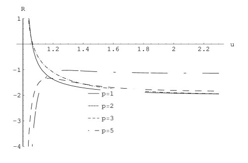
Figure 8: The curves show $\alpha^{\prime}\,R$ as a function of $\tilde{u}={u\over u_{0}}$ for different values of $p$, where $R$ is the scalar curvature of (5.29) for $a=1/5$ and $e=-3/10$.

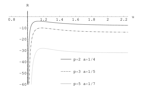
Figure 9: The curves show $\alpha^{\prime}\,R$ for (5.29) as a function of $\tilde{u}={u\over u_{0}}$ for different values of $p$. The values of $a$ and $e$ are such that the solutions satisfy the Maldacena-Nuñez criterion and have a bounded string coupling.

Among the members of the family, those with $a+p\,e+\frac{1}{p+2}\leq 0$ have a bounded string coupling everywhere. And, as it happened with the family of solutions of Section $3.2$, when the inequality is saturated, they are also regular. In fact, the scalar curvature of (5.29) reads,

$$l_{0}{}^{2}\,R = -\left(1+(p+2)\,(a+pe)\right)^{2}\;\frac{1}{f(u)}-(p-1)\,(p+2)+2-2\,(p+2)^{2}\;(a+pe)^{2}$$ (5.30)

$$- \left(1-(p+2)\,(a+pe)\right)^{2}\;f(u)$$ (5.31)

showing explicitly that the curvature is finite at $u\rightarrow u_{0}$ iff the condition $a+p\,e+\frac{1}{p+2}=0$ holds. In this case, the following two solutions emerge.

Solution 1. $a=-\frac{p+1}{p+2}\;\;,\;\;e=\frac{1}{p+2}$

$$G = l_{0}{}^{2}\;\left(-u^{2}\;f(u)\;dx^{0}{}^{2}+u^{2}\;d^{2}\vec{x}+\frac{1}{f(u)}\;\frac{du^{2}}{u^{2}}\right)+\frac{R_{0}{}^{2}}{(l_{0}\,u)^{2}}\;d\theta^{2}$$ (5.32)

$$e^{-2\Phi} = e^{-2\Phi_{0}}\;(l_{0}\,u)^{2}$$ (5.33)

$$F_{p+2} = s(q)\;2\,\sqrt{p+2}\;e^{-\Phi_{0}}\;l_{0}{}^{p+2}\;u^{p+1}\;du\wedge dx^{0}\wedge\dots\wedge dx^{p}$$ (5.34)

It is an $AdS$ like black hole solution, with a running dilaton. Furthermore, it is not difficult to see, following the standard recipe, that in the limit of $u\rightarrow u_{0}$ the euclidean space obtained from the Wick rotation $\tau\equiv i\,x^{0}$ is regular if we impose the periodicity,

$$\tau\sim\tau+\beta\qquad,\qquad\beta\equiv\frac{4\,\pi}{p+2}\,\frac{1}{u_{0}}$$ (5.35)

This is an usual fact in a kind of solutions that we associate to field theories at finite temperature $\beta^{-1}$ [3].

Solution 2. $a=\frac{p^{2}+2p-1}{(p+1)\,(p+2)}\;\;,\;\;e=-\frac{p+3}{(p+1)\,(p+2)}$

$$G = l_{0}{}^{2}\;\left(-\frac{u^{2}}{f(u)^{\frac{p-1}{p+1}}}\;dx^{0}{}^{2}+u^{2}\;f(u)^{\frac{2}{p+1}}\;d^{2}\vec{x}+\frac{1}{f(u)}\;\frac{du^{2}}{u^{2}}\right)+\frac{R_{0}{}^{2}}{(l_{0}\,u)^{2}}\;d\theta^{2}$$ (5.36)

$$e^{-2\Phi} = e^{-2\Phi_{0}}\;(l_{0}\,u)^{2}$$ (5.37)

$$F_{p+2} = s(q)\;2\,\sqrt{p+2}\;e^{-\Phi_{0}}\;l_{0}{}^{p+2}\;u^{p+1}\;du\wedge dx^{0}\wedge\dots\wedge dx^{p}$$ (5.38)

The $D1$-brane case is included in the Solution $1$ through a double Wick rotation, $x^{0}\rightarrow-i\,x^{1}\;,\;x^{1}\rightarrow i\,x^{0}$. We noticed that both solutions are supported by the same dilaton and $RR$ gauge fields, and have the same scalar curvature, which is displayed in Figure $10$.

Figure 10: The curves show $\alpha^{\prime}\,R$ as a function of $\tilde{u}={u\over u_{0}}$ for different values of $p$, where $R$ is the scalar curvature of (5.34) and (5.38).

5.3 $T$-duality.

By applying the rules for $T$-duality transformations (see i.e. [31] and references therein) along the coordinate $\theta$, we can generate from (5.29) another family of solutions. The solutions obtained in this section assumed the proportionality between the functions $f_{1}$ and $f_{2}$, equation (5.7); it is easy to see that this ansätz yields the relation $e^{2\Phi}\propto G_{\theta\theta}$, which in turns yields T-dual solutions with constant dilaton. We get,

$$G = l_{0}{}^{2}\left(-\frac{u^{2}}{f(u)^{a-\frac{1}{p+2}}}\;dx^{0}{}^{2}+\frac{u^{2}}{f(u)^{e-\frac{1}{p+2}}}\;d\vec{x}{}^{2}+\frac{1}{f(u)}\;\frac{du^{2}}{u^{2}}\right.$$ (5.39)

$$+ \left.\left(\frac{\alpha^{\prime}}{R_{0}}\right)^{2}\;f(u)^{a+p\,e+\frac{1}{p+2}}\;u^{2}\;d\theta^{2}\right)$$ (5.40)

$$e^{2\Phi} = \frac{16\,\pi^{2}\,\alpha^{\prime}\,\Lambda^{2}}{(p+3)\,Q_{p}{}^{2}}$$ (5.41)

$$F_{p+3} = s(q)\;2\,\sqrt{p+2}\;e^{-\Phi_{0}}\;\sqrt{\alpha^{\prime}}\;l_{0}{}^{p+2}\;u^{p+1}\;du\wedge dx^{0}\wedge\dots\wedge dx^{p}\wedge d\theta$$ (5.42)

$$\frac{p+1}{p+2} = 2\,a^{2}+p\,(p+1)\,e^{2}+2\,p\,a\,e$$ (5.43)

It can be showed that this is a family of Einstein spaces with Ricci tensor,

$$R_{mn}=-\frac{p+2}{l_{0}{}^{2}}\;G_{mn}$$ (5.44)

All the members are asymptotic at large $u\gg u_{0}$ to $AdS_{1,p+2}$ space (after identifying $x^{p+1}\equiv\frac{\alpha^{\prime}}{R_{0}}\,\theta$). In particular, the T-dual solution to (5.34) results the $AdS_{1,p+2}$ Schwarzchild black hole recently derived in [17], and used in [21], [24], as a model of four dimensional YM theory .

6 Conclusions and perspectives.

In this paper, we have considered $p$-brane solutions to the low energy gravity equations of motion of non critical type II string theories in $D=p+3$ dimensions. We have reduced the problem to the search for the general solution of the system given by equations (2.36), (2.39).

Firstly, we found all the possible uncharged vacuum solutions. Besides $p+1$ Minkowski space-time times the linear dilaton times $S^{1}$, we found the three parameter family of solutions (3.22), that includes the well-known $p+1$ Minkowski space-time times the cigar, and its T-dual $p+1$ Minkowski space-time times the trumpet. In a large region of the parameter space the string coupling remains bounded, and there is a two parameter subfamily that also has bounded scalar curvature.

We were also able to solve completely the problem for all the possible NSNS charged backgrounds, which for $p=1$ represent (the near horizon of) fundamental string solutions. Among the large amount of found solutions, we highlight the fundamental string solution embedded in the cigar vacuum (4.35), recently found in [16], a new solution (4.19) interpretable as a F1 embedded in the linear dilaton vacuum, and a regular two-parameter family asymptotic to $AdS_{1,2}\times S^{1}$.

With regard to RR charged $Dp$-brane solutions, we were able to find analytically a class of solutions obeying a particular constraint. It includes a constant curvature solution asymptotic in the UV to $AdS_{1,p+1}$, that shrinks to $AdS_{2}$ in the IR limit; it is T-dual to $AdS_{1,p+2}$. This solution first appears in [17] as the near horizon of a (numerically found) solution asymptotic to the linear dilaton vacuum. Furthermore, we found a three parameter family of solutions (5.29), that presumably correspond to the near horizon limit of a three parameter family of black $Dp$-brane solutions, embedded in the linear dilaton vacuum, solutions that do not obey our ansätz (5.7) in all the space-time. On the other hand, we conjecture that there should exist $Dp$- branes embedded in the cigar vacuum which are solutions of (2.36), that do not obey our ansätz in any region, and that correspond to those constructed as boundary states in references [32], [33], [34] . This is subject for future work.

The condition that the solutions of (5.29) have a small string coupling reads,

$$e^{2\Phi_{0}}\ll f(u)^{a+p\,e+\frac{1}{p+2}}\;(l_{0}\,u)^{2}$$ (6.1)

For the regular solutions $1$ and $2$ of Section $7$, this condition reduces to,

$$e^{2\Phi_{0}}\ll(l_{0}\,u_{0})^{2}$$ (6.2)

and their curvature is showed in Figure $10$. However, we can consider the region of parameters where $a+p\,e+\frac{1}{p+2}\neq 0$. In that case, the solution will present a curvature singularity in the IR limit, $u\rightarrow u_{0}{}^{+}$. There is, nevertheless, nothing new in the fact that SUGRA solutions one would like to interpret as gravity duals of some field theory in the IR, have curvature or string coupling singularities. A known example having a curvature singularity is the Klebanov-Tseytlin solution [35], the UV limit of the regular Klebanov-Strassler [37], that however is useful in discussing aspects of the dual $N=1$ gauge theory that depend on the UV behavior of the theory, like the chiral anomaly of the R-current [36]. More generically, singular solutions could be useful if they satisfy that $G_{00}$ does not increase as one approaches the singularity, according to the strong form of the Maldacena-Nuñez criterion [38] (see also [39]). For example, the solutions in Figure $9$ satisfy this criterion. On the other hand, if $a+p\,e+\frac{1}{p+2}>0$, the string coupling blows up in the IR and we should switch to its “S-dual” solution, whatever it means. In this respect, the connection of non critical theories with ten dimensional ones worked out in references [40], [41], [42], could be of help.

On the top of the questions that deserve further investigations, it certainly remains to explore the possibility of using (some of) the solutions (5.29) as gravity dual of gauge field theories, along the lines of references [21], [24], and in particular, to understand the role of the exponents on the field theory side. Probably the T-dual versions (5.43) are best settled to this end, because all of them have the same constant dilaton that, being $|Q_{p}|\sim N$, where $N$ is the number of $Dp$-branes (see the discussion in footnote $3$), is given by,

$$g_{s}=e^{\Phi}\sim\frac{1}{N}$$ (6.3)

So, for $N$ large enough, we can trust perturbative string theory for any solution of the family. Furthermore, the computation on the gravity side of the number of degrees of freedom (“entropy”) along the lines of [17] yields,

$$S_{gravity}\sim\frac{N^{2}}{\delta^{p+1}}$$ (6.4)

where $\delta$ is an IR cutoff, which is the result we expect for a $p+2$ dimensional gauge theory with UV cutoff $\delta^{-1}$ [43]. Finally, it can be shown [45] that if the parameters obeys the constraint,

$$a+e>\frac{2}{p+2}$$ (6.5)

then, according to the Wilson loop criterion [44], the theory is confining. We hope to present related results in a future publication [45].

Acknowledgments.

We would like to thank Juan Maldacena for a discussion in the very early stage of these investigations, Jan Troost for useful correspondence, and very specially Jorge Russo for reading the manuscript and making enlightening comments and suggestions.

Appendix A Some useful formulae.

Here we collect properties related with the ansätz for the fields assumed in Section $2.1$,

$$G = -A^{2}\;dx^{0}{}^{2}+\tilde{A}^{2}\;d{\vec{x}}{}^{2}+C^{2}\;d\rho^{2}+\tilde{C}^{2}\;dz^{2}\equiv\eta_{mn}\;\omega^{m}\;\omega^{n}$$ (A.1)

$$A_{p+1} = dx^{0}\wedge\dots\wedge dx^{p}\;E(\rho)$$ (A.2)

$$\Phi = \Phi(\rho)$$ (A.3)

where $\vec{x}$ is a $p$ dimensional vector, and we have introduced the vielbein $\omega^{n}$ and dual vector fields $e_{m}$, $e_{m}(\omega^{n})=\delta_{m}^{n}$, defined by,

$$\begin{array}[]{rclcrcl}\omega^{0}&=&A(\rho)\;dx^{0}&,&\;\;\;\;e_{0}&=&A(\rho)^{-1}\;\partial_{0}\cr\omega^{I}&=&\tilde{A}(\rho)\;dx^{I}&,&\;\;\;\;e_{I}&=&\tilde{A}(\rho)^{-1}\;\partial_{I}\qquad,\qquad I=1,\dots,p\cr\omega^{p+1}&=&C(\rho)\;d\rho&,&\;\;\;\;e_{p+1}&=&C(\rho)^{-1}\;\partial_{\rho}\cr\omega^{p+2}&=&\tilde{C}(\rho)\;dz&,&\;\;\;\;e_{p+2}&=&\tilde{C}(\rho)^{-1}\;\partial_{z}\end{array}$$ (A.8)

A.1 Connections.

As usual, the connections $\omega^{m}{}_{n}$ are completely determined by

• No torsion condition:                  $d\omega^{m}+{\omega^{m}}_{n}\wedge\omega^{n}=0$

• Metricity:                                   $\omega_{mn}\equiv\eta_{mp}\,\omega^{p}{}_{n}=-\omega_{nm}.$

From the direct computation of the coefficients ${\;\alpha^{m}}_{nl}$,

$$d\omega^{m}\equiv{1\over 2}{\alpha^{m}}_{nl}\;\omega^{n}\wedge\omega^{l}\;\;\;,\;\;\;{\alpha^{m}}_{nl}=-{\alpha^{m}}_{ln}$$ (A.9)

we get the connections in the form,

$$\omega_{mn}\equiv\omega_{mnl}\;\omega^{l}\qquad,\qquad\omega_{mnl}={1\over 2}(\alpha_{mnl}-\alpha_{lmn}+\alpha_{nlm})$$ (A.10)

We resume the non zero connections associated with the metric in (A.3),

$$\omega_{0p+1} = {\partial_{\rho}\ln A\over C}\;\omega_{0}=e_{p+1}(\ln A)\;\omega_{0}$$ (A.11)

$$\omega_{Ip+1} = {\partial_{\rho}\ln\tilde{A}\over C}\;\omega_{I}=e_{p+1}(\ln\tilde{A})\;\omega_{I}$$ (A.12)

$$\omega_{p+1,p+2} = -{\partial_{\rho}\ln\tilde{C}\over C}\;\omega_{p+2}=-e_{p+1}(\ln\tilde{C})\;\omega_{p+2}$$ (A.13)

A.2 Covariant derivatives.

We collect here covariant derivatives of interest related to the connections presented before. By definition,

$D_{m}(A_{n})\equiv e_{m}(A_{n})-\omega_{snm}\;A_{s}$

Because in our equations we have scalar functions of $\rho$, it is enough to know a few of them. Let $\phi(\rho)$ be an arbitrary scalar function; then we have the following non zero derivatives (contraction of indices is assumed),

$$D_{p+1}(\phi) = e_{p+1}(\phi)=\frac{1}{C}\,\partial_{\rho}\phi$$ (A.14)

$$D_{0}{}^{2}(\phi) = -\frac{1}{C^{2}}\;\partial_{\rho}\ln A\;\partial_{\rho}\phi$$ (A.15)

$$D_{I}D_{J}(\phi) = \delta_{IJ}\;e_{p+1}(\ln\tilde{A})\;e_{p+1}(\phi)$$ (A.16)

$$D_{p+1}{}^{2}(\phi) = \partial_{\rho}\left({\partial_{\rho}\phi\over C^{2}}\right)+\frac{1}{C^{2}}\;\partial_{\rho}\ln C\;\partial_{\rho}\phi$$ (A.17)

$$D_{p+2}{}^{2}(\phi) = \frac{1}{C^{2}}\;\partial_{\rho}\ln\tilde{C}\;\partial_{\rho}\phi$$ (A.18)

$$D^{2}(\phi) = \frac{1}{F_{1}}\;\partial_{\rho}\left(\frac{F_{1}}{C^{2}}\;\partial_{\rho}\phi\right)=\partial_{\rho}\left(\frac{\partial_{\rho}\phi}{C^{2}}\right)+\frac{1}{C^{2}}\;\partial_{\rho}\ln F_{1}\;\partial_{\rho}\phi$$ (A.19)

$$e^{b\xi}D(e^{-b\xi}\;\psi\;D(\phi)) = \frac{1}{F_{1}\,e^{-b\xi}}\;\partial_{\rho}\left(\frac{F_{1}\,e^{-b\xi}}{C^{2}}\;\psi\;\partial_{\rho}\phi\right)$$ (A.20)

where $F_{1}\equiv A\,\tilde{A}^{p}\,C\,\tilde{C}\;$, $\;\epsilon_{G}=dx^{0}\wedge dx^{1}\wedge\dots\wedge dx^{p}\wedge d\rho\wedge d\theta\;F_{1}\,$.

A.3 Curvature tensor.

By definition,

$$\Re_{mn}\equiv d\omega_{mn}+\omega_{mp}\wedge\omega^{p}{}_{n}=\frac{1}{2}\,\Re_{mnpq}\;\omega^{p}\wedge\omega^{q}$$ (A.22)

The computation yields,

$$\Re_{0I} = D_{0}{}^{2}(\ln\tilde{A})\;\omega_{0}\wedge\omega_{I}$$ (A.23)

$$\Re_{0p+1} = -{1\over{A}}{D_{p+1}}^{2}(A)\;\omega_{0}\wedge\omega_{p+1}$$ (A.24)

$$\Re_{Ip+1} = -{1\over{\tilde{A}}}D_{p+1}{}^{2}(\tilde{A})\;\omega_{I}\wedge\omega_{p+1}$$ (A.25)

$$\Re_{IJ} = -D_{p+1}(\ln\tilde{A})^{2}\;\omega_{I}\wedge\omega_{J}$$ (A.26)

$$\Re_{0p+2} = -\frac{1}{A}D_{p+2}{}^{2}(A)\;\omega_{0}\wedge\omega_{p+2}$$ (A.27)

$$\Re_{Ip+2} = -\frac{1}{\tilde{A}}D_{p+2}{}^{2}(\tilde{A})\;\omega_{I}\wedge\omega_{p+2}$$ (A.28)

$$\Re_{p+1p+2} = -{1\over{\tilde{C}}}D_{p+1}{}^{2}(\tilde{C})\;\omega_{p+1}\wedge\omega_{p+2}$$ (A.29)

A.4 Ricci tensor and Ricci scalar.

From (A.29), we get the following components of the Ricci tensor $R_{mn}\equiv\Re^{p}{}_{mpn}$,

$$R_{00} = D^{2}(\ln A)$$ (A.30)

$$R_{IJ} = -D^{2}(\ln\tilde{A})\;\delta_{IJ}$$ (A.31)

$$R_{p+1p+1} = -D^{2}(\ln C)-{1\over A}\partial_{\rho}\left({\partial_{\rho}A\over C^{2}}\right)-{p\over\tilde{A}}\partial_{\rho}\left({\partial_{\rho}\tilde{A}\over C^{2}}\right)+{1\over C}\partial_{\rho}\left({\partial_{\tilde{\rho}}C\over C^{2}}\right)-{1\over\tilde{C}}\partial_{\rho}\left({\partial_{\rho}\tilde{C}\over C^{2}}\right)$$ (A.32)

$$= -D^{2}(\ln C)-\frac{D_{p+1}{}^{2}(A)}{A}-p\,\frac{D_{p+1}{}^{2}(\tilde{A})}{\tilde{A}}+\frac{D_{p+1}{}^{2}(C)}{C}-\frac{D_{p+1}{}^{2}(\tilde{C})}{\tilde{C}}$$ (A.33)

$$+ \frac{1}{C^{2}}\;\partial_{\rho}\ln C\;\partial_{\rho}\ln\frac{F_{1}}{C^{2}}$$ (A.34)

$$R_{p+2p+2} = -D^{2}(\ln\tilde{C})$$ (A.35)

The curvature scalar results,

$$R = -{2\over C}\partial_{\rho}^{2}\left({1\over C}\right)-D(\ln A)^{2}-p\,D(\ln\tilde{A})^{2}-D(\ln C)^{2}-D(\ln\tilde{C})^{2}$$ (A.36)

$$- 2\,D^{2}(\ln F_{1})+D(\ln F_{1})^{2}$$ (A.37)

A.5 Strength field tensor.

With the ansätz in (2.12) for the $p+1$ form we get,

$$F_{p+2} = dx^{0}\wedge\dots\wedge dx^{p}\;\partial_{\rho}E(\rho)$$ (A.38)

$$\left(F_{p+2}\right)^{2}_{\mu\nu} = -{(\partial_{\rho}E)^{2}\over(A\,\tilde{A}^{p}\,C)^{2}}\;\eta_{\mu\nu}$$ (A.39)

$$\left(F_{p+2}\right)^{2}_{p+1p+1} = -{(\partial_{\rho}E)^{2}\over(A\,\tilde{A}^{p}\,C)^{2}}\;$$ (A.40)

The gauge contribution to the strength field tensor results,

$$T^{A}_{\mu\nu} = -\frac{2-b_{p}}{8}\;\frac{e^{(2+b_{p})\Phi}}{\left(A\,{\tilde{A}}^{p}\,C\right)^{2}}\;\;(\partial_{\rho}E)^{2}\;\eta_{\mu\nu}$$ (A.41)

$$T^{A}_{p+1p+1} = -\frac{2-b_{p}}{8}\;\frac{e^{(2+b_{p})\Phi}}{\left(A\,{\tilde{A}}^{p}\,C\right)^{2}}\;\;(\partial_{\rho}E)^{2}$$ (A.42)

$$T^{A}_{p+2p+2} = \frac{2+b_{p}}{8}\;\frac{e^{(2+b_{p})\Phi}}{\left(A\,{\tilde{A}}^{p}\,C\right)^{2}}\;\;(\partial_{\rho}E)^{2}$$ (A.43)

A.6 The equations of motion.

With the help of the precedent results for the Ricci tensor, strength field tensor, etc., the equations of motion (2.5) for the ansätz (2.12) can be recast in the following way,

$A$-equation

$$e^{2\Phi}D(e^{-2\Phi}D(\ln A))={2-b_{p}\over 8}\;{e^{(b_{p}+2)\Phi}\over(A{\tilde{A}}^{p}\,C)^{2}}\;(\partial_{\rho}E)^{2}$$ (A.44)

$\tilde{A}$-equation

$$e^{2\Phi}D(e^{-2\Phi}D(\ln\tilde{A}))={2-b_{p}\over 8}\;{e^{(b_{p}+2)\Phi}\over(A{\tilde{A}}^{p}\,C)^{2}}\;(\partial_{\rho}E)^{2}$$ (A.45)

$C$-equation

$$- e^{2\Phi}D(e^{-2\Phi}D(\ln C))={D_{p+1}{}^{2}(A)\over A}+p\,{D_{p+1}{}^{2}(\tilde{A})\over\tilde{A}}-{D_{p+1}{}^{2}(C)\over C}+{D_{p+1}{}^{2}(\tilde{C})\over\tilde{C}}$$ (A.46)

$$- 2\,D_{p+1}{}^{2}(\Phi)-\frac{1}{C^{2}}\;\partial_{\rho}\ln C\;\partial_{\rho}\ln\left({F_{1}\over C^{2}}e^{-2\Phi}\right)-\frac{2-b_{p}}{8}\;{e^{(b_{p}+2)\Phi}\over(A{\tilde{A}}^{p}\,C)^{2}}\;(\partial_{\rho}E)^{2}$$ (A.47)

$\tilde{C}$-equation

$$-e^{2\Phi}D(e^{-2\Phi}D(\ln\tilde{C}))={2+b_{p}\over 8}\;{e^{(b_{p}+2)\Phi}\over(A{\tilde{A}}^{p}\,C)^{2}}\;(\partial_{\rho}E)^{2}$$ (A.48)

$\Phi$-equation

$$e^{2\Phi}D(e^{-2\Phi}D(\ln e^{-2\Phi}))=\Lambda^{2}-(p+1)\,{2-b_{p}\over 8}\;{e^{(b_{p}+2)\Phi}\over(A\tilde{A}^{p}\,C)^{2}}\;(\partial_{\rho}E)^{2}$$ (A.49)

E-equation

$$-D\left(\frac{e^{b_{p}\Phi}}{(A{\tilde{A}}^{p})^{2}}\;D(E)\right)=(-)^{p}\,Q_{p}\;\frac{\delta^{2}_{\perp}}{F_{1}}$$ (A.50)

In the last one, the $E$-equation, we used the relation,

$$*F_{p+2}=(-)^{p}\;\frac{\tilde{C}^{2}}{F_{1}}\;\partial_{\rho}E\;dz$$ (A.51)

and assumed a source of the form $\,Q_{p}\,J_{p+1}$,

$$J_{p+1}^{01\dots p}=\frac{\delta^{2}_{\perp}}{\sqrt{-\det G}}=\frac{\delta^{2}_{G^{\perp}}}{A\,\tilde{A}^{p}}\;\;\longrightarrow\;\;J_{p+1}=-\delta^{2}_{G^{\perp}}\;\omega^{0}\wedge\dots\wedge\omega^{p}$$ (A.52)

where $G^{\perp}$ stands for the metric of the space where the flat $p$ brane is localized.

References

- [1] O. Aharony, S. S. Gubser, J. M. Maldacena, H. Ooguri and Y. Oz, Phys. Rept. 323, 183 (2000) [arXiv:hep-th/9905111], and references therein.
- [2] For a short review on some topics, see, J. D. Edelstein and R. Portugues, Fortsch. Phys. 54, 525 (2006) [arXiv:hep-th/0602021].
- [3] E. Witten, “Anti-de Sitter space, thermal phase transition, and confinement in gauge Adv. Theor. Math. Phys. 2, 505 (1998) [arXiv:hep-th/9803131].
- [4] A. M. Polyakov, Int. J. Mod. Phys. A 14, 645 (1999) [arXiv:hep-th/9809057].
- [5] A. M. Polyakov, Phys. Lett. B 103, 207 (1981).
- [6] A. M. Polyakov, Phys. Lett. B 103, 211 (1981).
- [7] P. H. Ginsparg and G. W. Moore, arXiv:hep-th/9304011.
- [8] N. Seiberg, Prog. Theor. Phys. Suppl. 102, 319 (1990).
- [9] D. Kutasov and N. Seiberg, Phys. Lett. B 251, 67 (1990).
- [10] E. Witten, Phys. Rev. D 44, 314 (1991).
- [11] R. Dijkgraaf, H. L. Verlinde and E. P. Verlinde, Nucl. Phys. B 371, 269 (1992).
- [12] G. Mandal, A. M. Sengupta and S. R. Wadia, Mod. Phys. Lett. A 6, 1685 (1991).
- [13] I. Bars and K. Sfetsos, Phys. Rev. D 46, 4510 (1992) [arXiv:hep-th/9206006].
- [14] J. M. Maldacena, Adv. Theor. Math. Phys. 2, 231 (1998) [Int. J. Theor. Phys. 38, 1113 (1999)] [arXiv:hep-th/9711200].
- [15] N. Itzhaki, J. M. Maldacena, J. Sonnenschein and S. Yankielowicz, Phys. Rev. D 58, 046004 (1998) [arXiv:hep-th/9802042].
- [16] A. R. Lugo and M. B. Sturla, Phys. Lett. B 637, 338 (2006) [arXiv:hep-th/0604202].
- [17] S. Kuperstein and J. Sonnenschein, JHEP 0407, 049 (2004) [arXiv:hep-th/0403254].
- [18] I. R. Klebanov and J. M. Maldacena, Int. J. Mod. Phys. A 19, 5003 (2004) [arXiv:hep-th/0409133].
- [19] M. Alishahiha, A. Ghodsi and A. E. Mosaffa, JHEP 0501, 017 (2005) [arXiv:hep-th/0411087].
- [20] F. Bigazzi, R. Casero, A. Paredes and A. L. Cotrone, Fortsch. Phys. 54, 300 (2006).
- [21] S. Kuperstein and J. Sonnenschein, JHEP 0411, 026 (2004) [arXiv:hep-th/0411009].
- [22] A lot of work in the literature is devoted to the WZW model, see for example, J. M. Maldacena and H. Ooguri, J. Math. Phys. 42, 2929 (2001) [arXiv:hep-th/0001053], and references therein.
- [23] E. Alvarez, C. Gomez, L. Hernandez and P. Resco, Nucl. Phys. B 603, 286 (2001) [arXiv:hep-th/0101181].
- [24] R. Casero, A. Paredes and J. Sonnenschein, JHEP 0601, 127 (2006) [arXiv:hep-th/0510110].
- [25] R. C. Myers, Phys. Lett. B 199, 371 (1987).
- [26] J. Polchinski, “String theory, vol. 1”, Cambridge University Press, Cambridge (1998).
- [27] I. Antoniadis, C. Bachas, J. R. Ellis and D. V. Nanopoulos, Phys. Lett. B 257, 278 (1991).
- [28] A. A. Tseytlin and C. Vafa, Nucl. Phys. B 372, 443 (1992) [arXiv:hep-th/9109048].
- [29] E. A. Bergshoeff, A. Collinucci, D. Roest, J. G. Russo and P. K. Townsend, Class. Quant. Grav. 22, 4763 (2005) [arXiv:hep-th/0507143].
- [30] E. Alvarez, C. Gomez and L. Hernandez, Nucl. Phys. B 600, 185 (2001) [arXiv:hep-th/0011105].
- [31] C. V. Johnson, arXiv:hep-th/0007170.
- [32] S. K. Ashok, S. Murthy and J. Troost, Nucl. Phys. B 749, 172 (2006) [arXiv:hep-th/0504079].
- [33] A. Fotopoulos, V. Niarchos and N. Prezas, JHEP 0510, 081 (2005) [arXiv:hep-th/0504010].
- [34] S. Murthy and J. Troost, JHEP 0610, 019 (2006) [arXiv:hep-th/0606203].
- [35] I. R. Klebanov and A. A. Tseytlin, Nucl. Phys. B 578, 123 (2000) [arXiv:hep-th/0002159].
- [36] I. R. Klebanov and M. J. Strassler, JHEP 0008, 052 (2000) [arXiv:hep-th/0007191].
- [37] I. R. Klebanov, P. Ouyang and E. Witten, Phys. Rev. D 65, 105007 (2002) [arXiv:hep-th/0202056].
- [38] J. M. Maldacena and C. Nuñez, Int. J. Mod. Phys. A 16, 822 (2001) [arXiv:hep-th/0007018].
- [39] S. S. Gubser, Adv. Theor. Math. Phys. 4, 679 (2002) [arXiv:hep-th/0002160].
- [40] A. Giveon, D. Kutasov and O. Pelc, JHEP 9910, 035 (1999) [arXiv:hep-th/9907178].
- [41] A. Giveon and D. Kutasov, JHEP 9910, 034 (1999) [arXiv:hep-th/9909110].
- [42] A. Giveon and D. Kutasov, JHEP 0001, 023 (2000) [arXiv:hep-th/9911039].
- [43] L. Susskind and E. Witten, arXiv:hep-th/9805114.
- [44] Y. Kinar, E. Schreiber and J. Sonnenschein, Nucl. Phys. B 566, 103 (2000) [arXiv:hep-th/9811192].
- [45] A. Lugo and M. Sturla, work in progress.