Simulations of astronomical imaging phased arrays

Abstract

We describe a theoretical procedure for analyzing astronomical phased arrays with overlapping beams, and apply the procedure to simulate a simple example. We demonstrate the effect of overlapping beams on the number of degrees of freedom of the array, and on the ability of the array to recover a source. We show that the best images are obtained using overlapping beams, contrary to common practise, and show how the dynamic range of a phased array directly affects the image quality.

1 Introduction

Phased arrays have had many applications in the field of radar. In recent years there has been a considerable increase of interest in radio astronomy applications, with such projects as the Square Kilometer Array (SKA) [4, 17], the Electronic Multibeam Radio Astronomy Concept (EMBRACE) [2], the Karoo Array Telescope (KAT), and the Low Frequency Array (LOFAR) [9]. Furthermore, there are plans to place phased arrays in the focal or aperture planes of single dish telescopes, and as technology improves, phased arrays will be utilized at submillimeter wavelengths in addition to the radio and microwave spectrum.

In designing phased arrays it has been standard practise to ensure that the synthesized beams are mathematically orthogonal, and thus when the incoming field matches one of the beam patterns precisely, only one port of the phased array is excited. Approximate (though not precise) orthogonality of the beams is technically straightforward to achieve, and simplifies the analysis, but, as we shall show, is not necessarily desirable. In particular, in order to achieve orthogonality one needs either to have the beams widely spaced, which leaves large parts of the sky uncovered, or to make the beams as narrow as possible, which increases the sidelobe levels. Recent work on shapelets [7, 6, 16, 3, 11] and other non–orthogonal functions suggest on the contrary that it is desirable for the beams to overlap, such that is not possible for an incoming field to give rise to a signal at one port alone.

In a previous paper [18], we developed a general theory for analysing phased arrays that allows overlapping beams to be modelled. The theory identifies the natural modes of a phased array, namely those orthogonal field patterns to which a phased array can couple, which will not in general be equivalent to the beam patterns. We showed how, once the modes have been identified, sources can be recovered from measured correlations, and noise can be incorporated into the model. The purpose of this paper is to develop the theory, illustrated by simulations, for a particular class of phased array: a regularly spaced array of identical, non–interacting, paraxial horns, equipped with a Butler matrix [12] to form the synthesized beams. The theory we developed previously is much more general, allowing for interaction between the horns, and for wide angle primary beams, as well as placing no restriction, other than linearity, on the type of beam combiner. In particular the theory permits the modelling of phased arrays of planar antennas, operating at short wavelengths. Additionally, extensive work has been done on reducing sidelobes by the use of non–uniform array configurations [8, 10]. Nevertheless, we restrict ourselves in this paper to the simplest type of phased array for two reasons. Firstly, the effects of overlapping beams on image recovery have not previously been fully appreciated, and we wish to demonstrate the effects in the simplest possible system. Secondly, although sidelobes can be reduced by the use of non–uniform arrays, there is still a well known tradeoff between beam width and sidelobe levels, so our results have implication for more sophisticated array geometries.

2 Theory

Consider an array of $M$ non–interacting horns. Let $\widehat{\boldsymbol{\Omega}}$ be the unit vector pointing in the direction of arrival (DoA) for each point on the sky, measured from a reference point in the aperture plane. Because $\widehat{\boldsymbol{\Omega}}$ is constrained to be of unit length, it has only 2 degrees of freedom, and the $x$ and $y$ components $\widehat{\Omega}^{x}$ and $\widehat{\Omega}^{y}$ are the angular coordinates in radians of the associated point on the sky (throughout the paper we use superscripts to denote the Cartesian components of a vector, and subscripts to index horns and ports). Let $\mathrm{d}\Omega$ be an infinitesimal patch of solid angle with DoA vector $\widehat{\boldsymbol{\Omega}}$, and let $\mathcal{A}$ be a patch of solid angle large enough to contain the primary beam (the beam of the horn). The signal at the $m$th horn is then given by

$$y_{m}=\int_{\mathcal{A}}\phi^{*}_{m}(\widehat{\boldsymbol{\Omega}})E(\widehat{\boldsymbol{\Omega}})\mathrm{d}\Omega\;,$$ (1)

where $\phi_{m}(\widehat{\boldsymbol{\Omega}})$ is the beam of the $m$th horn and $E(\widehat{\boldsymbol{\Omega}})$ is the magnitude of the component of the electric field arriving from direction $\widehat{\boldsymbol{\Omega}}$. In this paper we work in terms of scalar fields, for simplicity, but in our previous paper [18] we developed the theory in terms of vector fields, thus allowing polarization to be incorporated.

A phased array is formed by taking linear combinations of the signals from the horns. Assuming that there is no scattering from the beam forming network into the horns, or that any such scattering is linear, the signal at the $p$th port is

$$z_{p}=\sum_{m=1}^{M}S_{pm}y_{m}\;,\qquad p=1\to P\;,$$ (2)

where $S_{pm}$ is the scattering matrix of the beam forming network (which need not be square), and $P$ is the number of ports. We can thus define a synthesized beam $\psi_{p}(\widehat{\boldsymbol{\Omega}})$ associated with the $p$th port by

$$\psi_{p}(\widehat{\boldsymbol{\Omega}})=\sum_{m=1}^{M}S^{*}_{pm}\phi_{m}(\widehat{\boldsymbol{\Omega}})\;,$$ (3)

for then we can write the output of the $p$th port as

$$z_{p}=\int_{\mathcal{A}}\psi^{*}_{p}(\widehat{\boldsymbol{\Omega}})E(\widehat{\boldsymbol{\Omega}})\mathrm{d}\Omega$$ (4)

For partially coherent sources, we can write a similar result in terms of coherence functions:

$$\langle z_{p}z^{*}_{p^{\prime}}\rangle=\int_{\mathcal{A}}\int_{\mathcal{A}}\psi^{*}_{p}(\widehat{\boldsymbol{\Omega}}_{1})\psi_{p^{\prime}}(\widehat{\boldsymbol{\Omega}}_{2})\Gamma(\widehat{\boldsymbol{\Omega}}_{1},\widehat{\boldsymbol{\Omega}}_{2})\mathrm{d}\Omega_{1}\mathrm{d}\Omega_{2}\;,$$ (5)

where

$$\Gamma(\widehat{\boldsymbol{\Omega}}_{1},\widehat{\boldsymbol{\Omega}}_{2})\equiv\langle E(\widehat{\boldsymbol{\Omega}}_{1})E^{*}(\widehat{\boldsymbol{\Omega}}_{2})\rangle$$ (6)

is the mutual coherence function of the field on the sky. For most astronomical sources, $\Gamma(\widehat{\boldsymbol{\Omega}}_{1},\widehat{\boldsymbol{\Omega}}_{2})$ will be diagonal; however if the object being imaged is a maser, it will be spatially coherent, while if a phased array is placed in the focal plane of a telescope, even an incoherent source can give rise to coherent fields.

2.1 Image recovery

Suppose we have measured the outputs $z_{p}$ of a phased array and want to reconstruct the field on the sky. In our previous paper [18] we introduced the idea of using dual beams for this purpose: we now describe this method.

We showed that the beams $\psi_{p}(\widehat{\boldsymbol{\Omega}})$ can be decomposed thus:

$$\psi_{p}(\widehat{\boldsymbol{\Omega}})=\sum_{n}^{N}U^{*}_{pn}\sigma_{n}V_{n}(\widehat{\boldsymbol{\Omega}})\;,$$ (7)

where $\sigma_{n}$ is a real number greater than zero, $N$ is a finite integer, less than or equal to both the number of horns $M$ and the number of ports $P$, and $U_{pn}$ and $V_{n}(\widehat{\boldsymbol{\Omega}})$ satisfy the orthogonality relations

$$\int_{\mathcal{A}}V^{*}_{n}(\widehat{\boldsymbol{\Omega}})V_{n^{\prime}}(\widehat{\boldsymbol{\Omega}})\mathrm{d}\Omega = \delta_{nn^{\prime}}\;,$$ (8)

$$\sum_{p}^{P}U^{*}_{pn}U_{pn^{\prime}} = \delta_{nn^{\prime}}\;.$$ (9)

We have called $V_{n^{\prime}}(\widehat{\boldsymbol{\Omega}})$ the “eigenfields” in previous publications: they are an orthogonal and minimal set of functions the phased array can couple to, and can thus be considered to be its natural modes. In the parlance of the theory of continuous functions, (7) is known as a Hilbert–Schmidt decomposition. When the beams are discretized for numerical work, (7) becomes a singular value decomposition (SVD). The SVD has been used extensively in many applications, and there are numerous algorithms for its computation. Its two primary uses are in data compression and the calculation of generalized inverses; in this paper we use it in the latter capacity. We showed that the dual beams $\widetilde{\psi}_{p}(\widehat{\boldsymbol{\Omega}})$, analagous to the generalized inverse of a matrix [13, 14, 15] may be defined as

$$\widetilde{\psi}_{p}(\widehat{\boldsymbol{\Omega}})=\sum_{n}^{N}U^{*}_{pn}\sigma^{-1}_{n}V_{n}(\widehat{\boldsymbol{\Omega}})\;.$$ (10)

The incident field may then be estimated by

$$\widetilde{E}(\widehat{\boldsymbol{\Omega}})=\sum_{p}^{P}z_{p}\widetilde{\psi}_{p}(\widehat{\boldsymbol{\Omega}})\;.$$ (11)

(11) gives the best estimate of the incoming field in the sense that the error $E(\widehat{\boldsymbol{\Omega}})-\widetilde{E}(\widehat{\boldsymbol{\Omega}})$ is mathematically orthogonal to all of the eigenfields, the synthesized beams, and the dual beams. In the case that the beams span the incoming field then $\widetilde{E}(\widehat{\boldsymbol{\Omega}})=E(\widehat{\boldsymbol{\Omega}})$; if the beams span all possible incoming fields then we say that the beams constitute a frame [5].

In the case of the partially coherent field (5), the coherence of the incoming field can be estimated by

$$\widetilde{\Gamma}(\widehat{\boldsymbol{\Omega}}_{1},\widehat{\boldsymbol{\Omega}}_{2})=\sum_{p,p^{\prime}}^{P}\langle z_{p}z^{*}_{p^{\prime}}\rangle\widetilde{\psi}_{p}(\widehat{\boldsymbol{\Omega}})\widetilde{\psi}_{p^{\prime}}(\widehat{\boldsymbol{\Omega}})\;.$$ (12)

This is also a “best estimate” in the sense that the error $\widetilde{\Gamma}(\widehat{\boldsymbol{\Omega}}_{1},\widehat{\boldsymbol{\Omega}}_{2})-\Gamma(\widehat{\boldsymbol{\Omega}}_{1},\widehat{\boldsymbol{\Omega}}_{2})$ is orthogonal to any dyadic formed from the eigenfields. It is not however constrained to be incoherent. We have addressed this problem in [18], introducing the idea of “interferometric frames”, and we will develop the idea further in future publications; however we note that setting $\widehat{\boldsymbol{\Omega}}_{1}=\widehat{\boldsymbol{\Omega}}_{2}$ in (12) still provides a good estimate of the intensity distribution of the source, and indeed is numerically more efficient than the use of interferometric frames.

2.2 Array of identical paraxial horns with a Butler matrix

If the horns are identical, and their beams are sufficiently narrow to be described by paraxial optics, their beams can be trivially related to the beam of a single horn at an arbitrary reference position by

$$\phi_{m}(\widehat{\boldsymbol{\Omega}})=e^{i\boldsymbol{b}_{m}\cdot\widehat{\boldsymbol{\Omega}}}\phi(\widehat{\boldsymbol{\Omega}})\;,$$ (13)

where $\boldsymbol{b}_{m}$ is the displacement vector of the $m$th horn in wavelengths from the reference position, The normal choice of beam forming network is a Butler matrix, which can be represented by the scattering matrix

$$S_{pm}=e^{i\widehat{\boldsymbol{\alpha}}_{p}\cdot\boldsymbol{b}_{m}}\;,$$ (14)

and gives rise to the synthesized beams

$$\psi_{p}(\widehat{\boldsymbol{\Omega}})=\sum_{m=1}^{M}e^{-i\boldsymbol{b}_{m}\cdot(\widehat{\boldsymbol{\alpha}}_{p}-\widehat{\boldsymbol{\Omega}})}\phi(\widehat{\boldsymbol{\Omega}})\;,$$ (15)

where $\widehat{\boldsymbol{\alpha}}_{p}$ is a DoA unit vector chosen to move the synthesized beams around on the sky. Henceforth in this paper we consider only arrays for which $b_{m}^{z}=0$ and hence $\widehat{\Omega}^{z}$ and $\widehat{\alpha}_{p}^{z}$ can be ignored. In practice a Butler matrix can be constructed from a lossless combination of $90^{\circ}$ hybrid couplers and phase shifters [12]. The reason for using a Butler matrix is that the signal from the $p$th port is

$$z_{p}=\int_{\mathcal{A}}\sum_{m=1}^{M}e^{i\boldsymbol{b}_{m}\cdot(\widehat{\boldsymbol{\alpha}}_{p}-\widehat{\boldsymbol{\Omega}})}\phi^{*}(\widehat{\boldsymbol{\Omega}})E(\widehat{\boldsymbol{\Omega}})\mathrm{d}\Omega\;,$$ (16)

and, for an array with a sufficient number of horns,

$$z_{p}\to\phi^{*}(\widehat{\boldsymbol{\alpha}}_{p})E(\widehat{\boldsymbol{\alpha}}_{p}).$$ (17)

Thus, in the limit of perfect coverage, the signal from each port corresponds to a point on the sky, weighted by the conjugate of the primary beam. However for a real array, the synthesized beams have finite extent, so even with a simple Butler matrix it is straightforward to generate overlapping, non–orthogonal beams; indeed it is necessary to choose the spacing of the horns carefully if near–orthogonal beams are desired. We note that (16) is invariant under the simultaneous transformation

$$\widehat{\boldsymbol{\Omega}} \mapsto C\widehat{\boldsymbol{\Omega}}\;,$$

$$\widehat{\boldsymbol{\alpha}} \mapsto C\widehat{\boldsymbol{\alpha}}\;,$$

$$\boldsymbol{b} \mapsto \frac{1}{C}\boldsymbol{b}\;,$$ (18)

for some non–zero constant $C$. Thus the same behaviour is shown if we scale the baseline vectors in inverse proportion to the angular scales.

We now consider the detailed behaviour of the synthesized beams when the coverage is not perfect, in the sense that the Fourier components of the incident waves are not fully sampled. First we consider the case of a densely packed square array, with dimensions $B^{x}\times B^{y}$ wavelengths. In this case the summation in (15) can be approximated by an integral, resulting in the approximation

$$\psi_{p}(\widehat{\boldsymbol{\Omega}})\sim\textrm{sinc}(B^{x}(\widehat{\Omega}^{x}-\widehat{\alpha}_{p}^{x})/2)\textrm{sinc}(B^{y}(\widehat{\Omega}^{y}-\widehat{\alpha}_{p}^{y})/2)\phi(\widehat{\boldsymbol{\Omega}})\;.$$ (19)

Thus the spatial frequency of the sidelobes and the width of the central lobe of the beam are determined by the size of the array.

Now we consider an array that is less densely packed. The beam patterns will clearly be more complex, but the width of the central lobe and the typical spacing of the sidelobes are expected still to be determined largely by the overall array size. Another effect of the sampling however is to introduce grating lobes. If the position vector of the $p$th horn can be written in the form

$$\boldsymbol{b}_{p}=n_{p}^{1}\Delta b^{1}\boldsymbol{e}_{1}+n_{p}^{2}\Delta b^{2}\boldsymbol{e}_{2}$$ (20)

where $n_{p}^{1}$ and $n_{p}^{2}$ are integers and $\{\boldsymbol{e}_{1},\boldsymbol{e}_{2}\}$ is a set of lattice vectors, then from (15) and (20) we see that

$$\frac{\psi_{p}(\widehat{\boldsymbol{\Omega}})}{\phi(\widehat{\boldsymbol{\Omega}})}=\frac{\psi_{p}(\widehat{\boldsymbol{\Omega}}+m^{1}\frac{2\pi}{\Delta b^{1}}\boldsymbol{\tilde{e}}_{1}+m^{2}\frac{2\pi}{\Delta b^{2}}\boldsymbol{\tilde{e}}_{2})}{\phi(\widehat{\boldsymbol{\Omega}}+m^{1}\frac{2\pi}{\Delta b^{1}}\boldsymbol{\tilde{e}}_{1}+m^{2}\frac{2\pi}{\Delta b^{2}}\boldsymbol{\tilde{e}}_{2})}$$ (21)

for all integers $m^{1}$ and $m^{2}$, where $\{\boldsymbol{\tilde{e}}_{1},\boldsymbol{\tilde{e}}_{2}\}$ is the reciprocal basis satisfying $\boldsymbol{\tilde{e}}_{i}\cdot\boldsymbol{e}_{j}=\delta_{ij}$. The periodicity depends thus on the minimum spacing between horns, not on the overall size of the array, and furthermore does not require the grid of horns to be square or indeed for all positions on the grid to be filled. If the position vectors of the horns cannot be written in the form (20), the strict periodicity will not be seen; nevertheless, significant sidelobes are still likely.

To summarize, we expect to see the following features in the synthesized beams of a regular square array of size $B$ wavelengths and spacing $\Delta B$ wavelengths:

1. A principal lobe of width $\sim\frac{2\pi}{B}$

2. Sidelobes with typical spacing $\sim\frac{2\pi}{B}$

3. Grating lobes with spacing $\sim\frac{2\pi}{\Delta b}$

We have discussed the properties of the synthesized beams; now we discuss practical issues relating to their use. In the past, the approach has been to make the synthesized beams near–orthogonal, but the effect of this is to leave large gaps on the sky that are not covered by any beam, and additionally to increase the level of the sidelobes. As we shall demonstrate, this is an unnecessary restriction on the design of phased arrays, and indeed it is desirable that overlapping beams should be used.

3 Numerical results and discussion

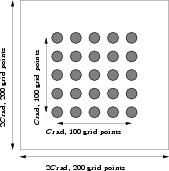
Figure 1: Positions of the sythesized beams on the sky

In this section we simulate phased arrays consisting of a square array of identical non–interacting horns, with Gaussian beam patterns, and equipped with Butler matrices as described in Section 2.2, the beams being given by (15). We use the rescaling given in (2.2). The phase slopes $\widehat{\boldsymbol{\alpha}}_{p}$ are chosen such that the centers of the beams form a square grid of dimension $C$ radians, while the grid used for the numerical integrations has dimension $2C$ radians, and $200\times 200$ grid points (see Figure 1). The horns have Gaussian beams with width $0.5C$ radians. The left hand panel of Figure 2 shows the beam of the horns. The dual beams were obtained from (7) and (10), using the LAPACK [1] “divide and conquer” routine to perform the SVD. In calculating the duals, singular values below one part in $10^{5}$ of the largest singular value were discarded, corresponding to a dynamic range of 100dB. In addition to finding the beams, duals and singular value decomposition, we tested the ability of the array to recover both a fully coherent and a fully incoherent source, using equation (11) and (12) respectively. The test source used is shown in the right hand panel of Figure 2.

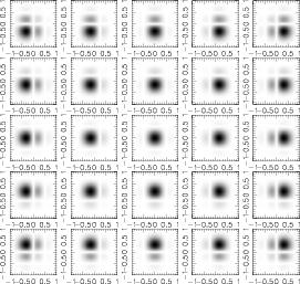
Figure 3: Linear grayscale plots showing the magnitude, as a function of $\widehat{\Omega}^{x}/C$ and $\widehat{\Omega}^{y}/C$, of the synthesized beams of an array with $5\times 5$ horns, total size $10\times 10/C$ wavelengths

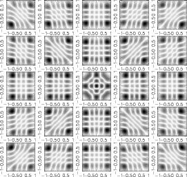
Figure 4: Linear grayscale plots showing the magnitude, as a function of $\widehat{\Omega}^{x}/C$ and $\widehat{\Omega}^{y}/C$, of the dual beams of an array with $5\times 5$ horns, total size $10\times 10/C$ wavelengths

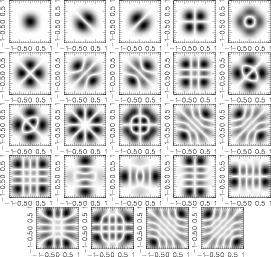
Figure 5: Linear grayscale plots showing the magnitude, as a function of $\widehat{\Omega}^{x}/C$ and $\widehat{\Omega}^{y}/C$, of the eigenfields of an array with $5\times 5$ horns, total size $10\times 10/C$ wavelengths

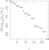
Figure 6: Singular values in dB of an array with$5\times 5$ horns, total size $10\times 10/C$ wavelengths

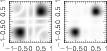
Figure 7: Linear grayscale plots showing the magnitude of a reconstructed coherent source (left), and the intensity of a reconstructed incoherent source (right), as a function of $\widehat{\Omega}^{x}/C$ and $\widehat{\Omega}^{y}/C$, for an array with $5\times 5$ horns, total size $10\times 10/C$ wavelengths

Figures 3 and 4 show the beams and dual beams of a phased array with a square grid of $5\times 5$ horns, of overall size $10/C$ wavelengths, and with $5\times 5$ synthesized beams such that $P=M$. The key features in the synthesized beams are the central maximum, which moves across the sky as $\widehat{\boldsymbol{\alpha}}_{p}$ is varied, and the large sidelobes. As would be expected from the form of the beams, they are far from orthogonal, and the dual beams take a very different form to the beams. Figures 5 and 6 show the corresponding eigenfields (which are the natural modes) and singular values; the singular values are plotted in decibels, normalized to the largest singular value. There are fewer eigenfields than synthesized beams because some of the singular values are below the dynamic range of 100dB below the largest singular value. Note that the lower order eigenfields bear some resemblance to prolate spheroidal wavefunctions, but the higher order ones exhibit unusual and complex geometries. Note also that the integral operator describing the phased array is poorly conditioned but non–singular, because the number of horns is equal to the number of ports. In Figure 7 we show reconstructed fully and mutually coherent and incoherent fields obtained from the array. They have similar features, except that the artefacts are more prominent in the coherent case. We observe the physical significance of the dual beams: their geometry characterizes the artefacts obtained when a reconstruction of the field is performed using the SVD.

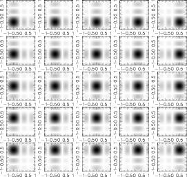
Figure 8: Linear grayscale plots showing the magnitude, as a function of $\widehat{\Omega}^{x}/C$ and $\widehat{\Omega}^{y}/C$, of the synthesized beams of an array with $5\times 5$ horns, total size $10\times 10/C$ wavelengths, and uniform primary beams

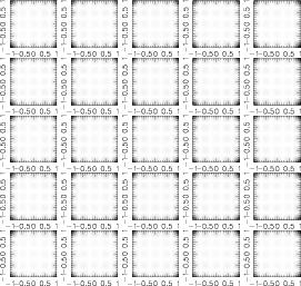
Figure 9: Linear grayscale plots showing the magnitude, as a function of $\widehat{\Omega}^{x}/C$ and $\widehat{\Omega}^{y}/C$, of the dual beams of an array with $5\times 5$ horns, total size $10\times 10/C$ wavelengths, and uniform primary beams

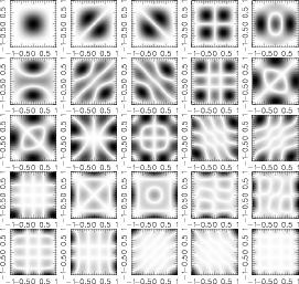
Figure 10: Linear grayscale plots showing the magnitude, as a function of $\widehat{\Omega}^{x}/C$ and $\widehat{\Omega}^{y}/C$, of the eigenfields of an array with $5\times 5$ horns, total size $10\times 10/C$ wavelengths, and uniform primary beams

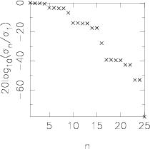
Figure 11: Singular values in dB of an array with$5\times 5$ horns, total size $10\times 10/C$ wavelengths, and uniform primary beams

The synthesized beams depend on both the geometry of the array and the form of the primary beams. To separate these effects we show the beams, dual beams, eigenfields and spectrum of the same phased array as above but with a uniform primary beam. Clearly this is not physically realistic, but it serves to demonstrate the role of the primary beam. The results are shown in Figures 8, 9, 10 and 11. When we compare these results with those obtained with a Gaussian primary beam, we observe that the Gaussian beam has the effect of truncating the synthesized beams at the edges, as expected. An effect of this is to shift the maxima in the sythesized beams towards the center, i.e. the maximum of the $p$th synthesized beams is not in fact at the vector $\widehat{\boldsymbol{\alpha}}_{p}$. The dual beams take a much simpler form without the primary beam; indeed they differ from each other only in the phases, as the amplitudes are all the same. The spectrum shows that the matrix is better conditioned when the primary beam is uniform; this is not surprising as information is expected to be lost when the beams are tapered. The lower order singular vectors are of similar form whether the primary beam is uniform or not, and are merely tapered at the edges by the primary beam; the higher order singular vectors are quite different. This would be expected because, for a tapered beam, the higher order singular vectors are concentrated away from the center.

3.1 Variable number of horns, fixed array size

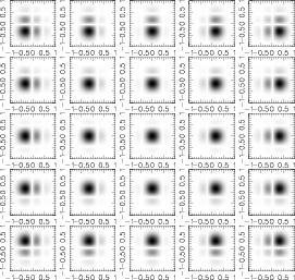
Figure 12: Linear grayscale plots showing the magnitude, as a function of $\widehat{\Omega}^{x}/C$ and $\widehat{\Omega}^{y}/C$, of the synthesized beams of an array with $4\times 4$ horns, total size $10\times 10/C$ wavelengths

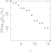
Figure 13: Singular values in dB of an array with $4\times 4$ horns, total size $10\times 10/C$ wavelengths

Now we consider the effect of changing the number of horns, while keeping the size of the array and number of ports fixed. We revert to the Gaussian primary beam. Figures 12 and 13 show the synthesized beams and spectrum for an array with 16 horns in a $4\times 4$ grid (for which $P>M$); we see that the spectrum is truncated to 16 singular values. This is a different effect to the poor conditioning resulting from the overlapping beams seen previously, for here the spectrum falls strictly to zero. Thus the number of horns places an absolute restriction on the number of degrees of freedom of the phased array, while the beam overlap imposes a restriction depending on the dynamic range, which in turn depends on a number of factors including the noise levels. The effect of the reduced number of horns is manifest in the increased magnitude and higher spatial frequency of the sidelobes of the synthesized beams. The higher spatial frequency might be expected from the fact that the gaps between horns are larger, but we observe that this is only evident when the number of horns is fewer than the number of ports.

We also increased the number of horns to $10\times 10$ (such that $P<M$), and found that the results were identical to those with $5\times 5$ ports (data not shown). This can be explained by the fact that the maximum number of degrees of freedom is dictated by the smaller of the number of ports and the number of horns; there is therefore no advantage in increasing the number of horns above the number of ports.

3.2 Variable array size, fixed number of horns

Now we consider the effect of changing the size of the array, while maintaining the same number of horns. We revert to the original number of horns, in a $5\times 5$ array, but with the array dimensions halved. Figures 14 , 15, and 16 show the beams, duals and spectrum of such an array. The size of the synthesized beams increases, while the spatial frequency of sidelobes reduces so much that they are outside the primary beam, as would be expected. The dual beams take on a more complicated and less symmetric form. The spectrum falls more rapidly, as expected from the strongly overlapping beams. Remarkably, it is still possible to recover images with such an array, as shown in Figure 17. Again, the reconstructed fields contain artefacts resembling the dual beams. In practise the quality of image recovery is limited by the dynamic range of the system, as we shall show in Section 3.3.

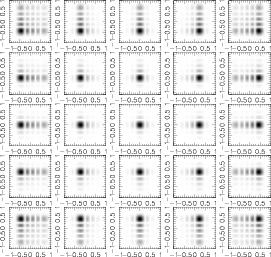
Figure 18: Linear grayscale plots showing the magnitude, as a function of $\widehat{\Omega}^{x}/C$ and $\widehat{\Omega}^{y}/C$, of the synthesized beams of an array with $5\times 5$ horns, total size $20\times 20/C$ wavelengths

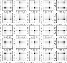
Figure 19: Linear grayscale plots showing the magnitude, as a function of $\widehat{\Omega}^{x}/C$ and $\widehat{\Omega}^{y}/C$, of the dual beams of an array with $5\times 5$ horns, total size $20\times 20/C$ wavelengths

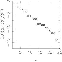
Figure 20: Singular values in dB of an array with $5\times 5$ horns, total size $20\times 20/C$ wavelengths

Now we increase the size of the array, again keeping the number of horns constant. Figures 18 and 19 shows the synthesized beams and duals for an array of twice the original dimensions, while Figure 20 shows the spectrum. We see that as the array size is increased the beams get smaller, and the frequency of the sidelobes increases. The beams also become more orthogonal, such that the duals closely resemble the beams, and the conditioning also improves. However, the reconstructed images in Figure 21 are of poor quality, and appear to be inferior to those obtained with the strongly overlapping beams in Figure 17. The reason is clear: in order to make the central lobes of the synthesized beams narrow enough that the beams are orthogonal, it is necessary to increase the frequency of the sidelobes, thus introducing artefacts into the reconstructed field. Moreover, the higher the frequency of the the sidelobes, the greater their intensity relative to the main lobe, and hence the greater the difficulty in deconvolving the image will be.

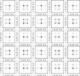
Figure 22: Linear grayscale plots showing the magnitude, as a function of $\widehat{\Omega}^{x}/C$ and $\widehat{\Omega}^{y}/C$, of the synthesized beams of an array with $5\times 5$ horns, total size $40\times 40/C$ wavelengths

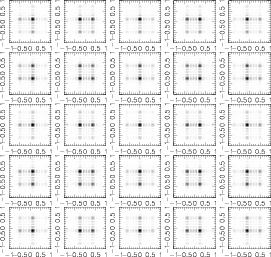
Figure 23: Linear grayscale plots showing the magnitude, as a function of $\widehat{\Omega}^{x}/C$ and $\widehat{\Omega}^{y}/C$, of the dual beams of an array with $5\times 5$ horns, total size $40\times 40/C$ wavelengths: duals

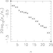
Figure 24: Singular values in dB of an array with $5\times 5$ horns, total size $40\times 40/C$ wavelengths

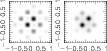
Figure 25: Linear grayscale plots showing the magnitude of a reconstructed coherent source (left), and the intensity of a reconstructed incoherent source (right), as a function of $\widehat{\Omega}^{x}/C$ and $\widehat{\Omega}^{y}/C$, for an array with $5\times 5$ horns, total size $40\times 40/C$ wavelengths

Figures 22, 23 and 24 show the beams, duals and spectrum of an array of 4 times the original dimensions, and the same effects are seen as in Figures 18–20, only more exaggerated. In addition however we see the periodicity in the synthesized beams discussed in Section 2.2, and furthermore the principle maxima in the beams are located in the middle, not at the “correct”, positions, as a result of truncation by the primary beam. This leads to aliasing, and hence to the completely erroneous reconstructed fields in Figure 25.

3.3 Dynamic range

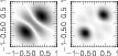
Figure 26: Linear grayscale plots showing the magnitude of a reconstructed coherent source (left), and the intensity of a reconstructed incoherent source (right), as a function of $\widehat{\Omega}^{x}/C$ and $\widehat{\Omega}^{y}/C$, for an array with $5\times 5$ horns, total size $5\times 5/C$ wavelengths, and dynamic range 50dB

The threshold below which singular values must be discarded, which dicates the value of $N$ in (7), is determined by the dynamic range of the system. In the preceding simulations we have used an implied dynamic range of 100dB; we now consider the effect of reducing this to 50dB. In Figure 26 we show the reconstructed fields obtained with this reduced dynamic range for the array of dimensions $5/C$ wavelengths used in Figure 17. We see that the reconstructed coherent field is of inferior quality with the reduced dynamic range. At first sight, the reconstructed incoherent field appears not to be so bad, but on closer inspection we see that the maxima have been shifted towards the center of the image, and away from their true position. This is because the discarded eigenfields are concentrated away from the center and thus contain the necessary information to correctly determine the position of the source. The dynamic range of the instrument is thus crucially important in determining the quality of the reconstructed image. The question we now ask is whether, in the case of limited dynamic range, we can improve the situation by synthesizing more beams.

3.4 Increasing number of synthesized beams

We now examine whether increasing the number of synthesized beams for a given configuration of horns makes any difference to the ability of the array to recover a field. We performed simulations for an array of dimension $5/C$, like that used in Figures 14–17, but with 100 synthesized beams in a $10\times 10$ grid covering the same patch of sky. The results were unchanged to Figures 14–17 (data not shown). Even when the dynamic range is reduced to 50dB, there is no difference obtained by using more beams.

We also consider whether increasing the number of beams has an effect for the array of dimension $20/C$, as used in Figure 21. In this case, the rank is equal to the number of horns; the question is whether the sidelobes can be removed by synthesizing more beams. Increasing the number of ports to 100 once again made no difference; our results strongly suggest that there is no advantage, at least in terms of modal throughput, in making the number of ports different to the number of horns.

4 Conclusion

We have performed simulations of imaging phased arrays, using our previously developed theory to calculate eigenfields and dual beams, and to reconstruct both coherent and incoherent test sources. The beam patterns show all the features one would expect for beams produced by a Butler matrix; the dual beams show complicated behaviour that results in artefacts in the reconstructed sources.

We have demonstrated that mathematically orthogonal beams do not give the best image quality, due to the inevitably increased sidelobe frequency. On the contrary some degree of overlap is desirable; however the overlap should ideally not be so much that the range of singular values exceeds the dynamic range of the system, as this degrades the image. We have looked for and failed to find any advantage in making the number of horns different to the number of ports.

The significance for the design of imaging phased arrays seems to be that, as a general rule, the number of ports should equal the number of horns, and that the beams should be made to overlap as much as the dynamic range of the instrument permits. It follows that improving the dynamic range of a phased array, by reducing noise for instance, will improve the quality of the images not only by reducing the noise in the image, but also by reducing the artefacts.

Figure 2: Linear grayscale plots showing the magnitude, as a function of $\widehat{\Omega}^{x}/C$ and $\widehat{\Omega}^{y}/C$, of the primary beam (left) and test source (right) used in the subsequent simulations

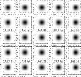
Figure 14: Linear grayscale plots showing the magnitude, as a function of $\widehat{\Omega}^{x}/C$ and $\widehat{\Omega}^{y}/C$, of the synthesized beams of an array with $5\times 5$ horns, total size $5\times 5/C$ wavelengths

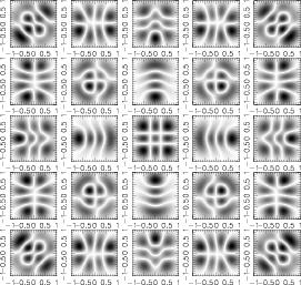
Figure 15: Linear grayscale plots showing the magnitude, as a function of $\widehat{\Omega}^{x}/C$ and $\widehat{\Omega}^{y}/C$, of the synthesized beams of an array with $5\times 5$ horns, total size $5\times 5/C$ wavelengths

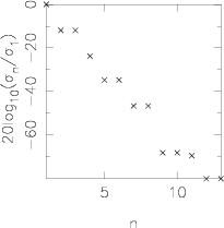
Figure 16: Singular values in dB of an array with $5\times 5$ horns, total size $5\times 5/C$ wavelengths

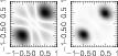
Figure 17: Linear grayscale plots showing the magnitude of a reconstructed coherent source (left), and the intensity of a reconstructed incoherent source (right), as a function of $\widehat{\Omega}^{x}/C$ and $\widehat{\Omega}^{y}/C$, for an array with $5\times 5$ horns, total size $5\times 5/C$ wavelengths

Figure 21: Linear grayscale plots showing the magnitude of a reconstructed coherent source (left), and the intensity of a reconstructed incoherent source (right), as a function of $\widehat{\Omega}^{x}/C$ and $\widehat{\Omega}^{y}/C$, for an array with $5\times 5$ horns, total size $20\times 20/C$ wavelengths

References

- [1] E. Anderson, Z. Bai, C. Bischof, S. Blackford, J. Demmel, J. Dongarra, J. Du Croz, A. Greenbaum, S. Hammarling, A. McKenney, and D. Sorensen. LAPACK Users’ Guide. Society for Industrial and Applied Mathematics, Philadelphia, PA, third edition, 1999.
- [2] A. Ardenne, P. Wilkinson, P. Patel, and J. Vaate. Electronic multi–beam radio astronomy concept: Embrace a demonstrator for the european ska program. Exp. Astron., 17:65–77, 2004.
- [3] R. H. Berry, M. P. Hobson, and S. Withington. Modal decomposition of astronomical images with application to shapelets. MNRAS, 354:199–211, 2004.
- [4] R. Braun. The concept of the square kilometer array interferometer. Proc. High Sensitivity Rad. Astron., pages 260–268, 1997.
- [5] P. G. Casazza. The art of frame theory. Taiwanese J. Math., 4:129–201, 2000.
- [6] I. Daubechies. The wavelet transform, time–frequency localization and signal analysis. IEEE Trans. Inform. Theory, pages 961–1005, 1990.
- [7] I. Daubechies, A. Grossmann, and Y. Meyer. Painless nonorthogonal expansions. J. Math. Phys., 27:1271–1283, 1986.
- [8] S. W. Ellingson. Efficient multibeam synthesis with interference nulling for large arrays. Trans. Antennas Propag., 51:503–511, 2003.
- [9] N. E. Kassim, T. J. W. Lazio, P. S. Ray, P. C. Crane, B. C. Hicks, K. P. Stewart, A. S. Cohen, and W. M. Lane. The low–frequency array (lofar): opening a new window on the universe. Planetary Space Sci., 52(15):1543–1549, 2004.
- [10] C. Lee, D. Leigh, and M. et al. Very fast subarray position calculation for minimizing sidelobes in sparse linear phased arrays. Proc. Eur. Conf. Antennas Propag., page 80.1, 2006.
- [11] R. Masset and A. Refregier. Polar shapelets. MNRAS, 363:197–210, 2005.
- [12] L. Milner and M. Parker. A broadband 8–18ghz 4–input 4–output butler matrix. Proc. SPIE, 6414:641406, 2007.
- [13] E. H. Moore. On the reciprocal of the general algebraic matrix. Bull. Am. Math. Soc., 26:394–395, 1920.
- [14] R. Penrose. A generalized inverse for matrices. Proc. Cambridge Phil. Soc., 51:406–413, 1955.
- [15] R. Penrose. On best approximate solutions of linear equations. Proc. Cambridge Phil. Soc., 52:17–19, 1955.
- [16] A. Refregier. Shapelets: A method for image analysis. MNRAS, 338:35–47, 2003.
- [17] A. van Ardenne, A. Smolders, and G. Hampson. Active adaptive antennas for radio astronomy: Results of the r & d program towards the square kilometer array. Proc. SPIE, 4015, 2000.
- [18] S. Withington, G. Saklatvala, and M. P. Hobson. Theoretical Analysis of Astronomical Phased Arrays. Submitted to J. Opt. A: Pure Appl. Opt., ArXiv e-prints, 707, July 2007.