Relationship between clustering and algorithmic phase transitions in the random k-XORSAT model and its NP-complete extensions

Abstract

We study the performances of stochastic heuristic search algorithms on Uniquely Extendible Constraint Satisfaction Problems with random inputs. We show that, for any heuristic preserving the Poissonian nature of the underlying instance, the (heuristic-dependent) largest ratio $\alpha_{a}$ of constraints per variables for which a search algorithm is likely to find solutions is smaller than the critical ratio $\alpha_{d}$ above which solutions are clustered and highly correlated. In addition we show that the clustering ratio can be reached when the number $k$ of variables per constraints goes to infinity by the so-called Generalized Unit Clause heuristic.

1 Introduction

The application of statistical mechanics ideas and tools to random optimization problems, initiated in the mid-eighties [1], has benefited from a renewed interest from the discovery of phase transitions in Constraint Satisfaction Problems (CSP) fifteen years ago. Briefly speaking, one wants to decide whether a set of randomly drawn constraints over a set of variables admits (at least) one solution. When the number of variables goes to infinity at fixed ratio $\alpha$ of constraints per variable the answer abruptly changes from (almost surely) Yes to No when the ratio crosses some critical value $\alpha_{s}$. Statistical physics studies have pointed out the existence of another phase transition in the Yes region [2, 3]. The set of solutions goes from being connected to a collection of disconnected clusters at some ratio $\alpha_{d}<\alpha_{s}$, a translation in optimization terms of the replica symmetry breaking transition identified by Parisi in mean-field spin glass theory.

It is expected that this clustering transition may have dynamical consequences. As replica symmetry breaking signals a loss of ergodicity, sampling algorithms (e.g. Monte Carlo procedure) run into problems at that transition. A quantitative study of the slowing down of MC scheme was done in [4] for the case of the $k$-XORSAT model where constraints are simply linear equations (modulo 2) over $k$ Boolean variables (for an introduction, see [5] and references therein). Yet, finding a solution should in principle be easier than sampling, and the exact nature of the relationship between the performances of resolution algorithms and the static phase transitions characterizing the solution space is far from being obvious [6]. The present paper is a modest step in elucidating this question for the $k$-XORSAT problem, and some related NP-complete problems sharing the same random structure.

Hereafter we consider simple stochastic search heuristic algorithms working in polynomial (linear) time for solving $k$-XORSAT instances [8, 5]. By successively assigning variables according to some heuristic rules those algorithms either produce a solution, or end up with a contradiction. The probability that a solution is found is a decreasing function of the ratio $\alpha$, and vanishes above some heuristic-dependent ratio $\alpha_{a}$ in the infinite size limit. We show that $\alpha_{a}<\alpha_{d}$ for any assignment heuristic in the class of rules preserving the Poissonian structure of the instance. In addition, we determine the most efficient heuristic, that is, the one maximizing $\alpha_{a}$ in this class and show that for large $k$, the two critical ratios match, $\alpha_{a}(k)\simeq\alpha_{d}(k)\simeq\log k/k$.

The plan of the paper is as follows. In section 2 we define the random $k$-XORSAT decision problem and its extension, as well as the search algorithms studied. Section 3 presents a method to characterize the phase diagrams of those random decision problems, depending on the content (numbers of constraints over $j$ variables, with $j$ ranging from 1 to $k$) of their instances. We show that all important information is encoded in a unique ‘thermodynamical’ potential for the fraction of frozen variables (backbone). The analysis of the dynamical evolution of the instance content is exposed in section 4. These dynamical results are combined with the static phase diagram in section 5 to show that the success-to-failure critical ratio of search heuristic, $\alpha_{a}$, is smaller than the ratio corresponding to the onset of clustering and large backbones, $\alpha_{d}$. We then show that the so-called Generalized Unit Clause heuristic rule is optimal (in the class of Poissonian heuristics) and its critical ratio $\alpha_{a}$ is asymptotically equal to $\alpha_{d}$ in the large $k$ limit. Our results are discussed in section 6.

2 Definitions

2.1 Decision problems

The decision problems we consider in this paper are $(k,d)$-Uniquely Extendible (UE) Constraint Satisfaction Problems (CSP) defined as follows [7]. One considers $N$ variables $x_{i}\in\{0,1,\cdots,d-1\}$. A UE constraint, or clause, is a constraint on $k$ variables such that, if one fixes a subset of $k-1$ variables, the value of the $k$-th variable is uniquely determined. A $(k,d)$-UE-CSP formula is a collection of $M=\alpha N$ clauses, each involving $k$ variables (out of the $N$ available ones). A solution is an assignment of the $N$ variables such that all the clauses are satisfied. $k$-XORSAT corresponds to $d=2$ and is solvable in polynomial time with standard linear algebra techniques. For $d=3$ the problem is still in P, while for $d\geq 4$ it has been shown that $(3,d)$-UE-CSP is NP-complete [7].

A random formula is obtained by choosing, for each clause, the $k$ variables, and the actual UE constraint, uniformly at random. It is known that, in the infinite size limit $N\rightarrow\infty$ and at fixed clause-to-variable ratio $\alpha$, [7, 11, 12, 13]:

• there is a critical ratio $\alpha_{s}(k)$ such that a random $(k,d)$-UE-CSP is almost surely satisfiable (respectively, unsatisfiable) if $\alpha<\alpha_{s}(k)$ (respectively, $\alpha>\alpha_{s}(k)$).

• in the satisfiable phase there is another phase transition at some ratio $\alpha_{d}(k)$ such that:

  - for $\alpha<\alpha_{d}(k)$ the space of solutions is ‘connected’: with high probability there is a path in the set of solutions joining any two solutions such that a step along the path requires to change O(1) variables.

  - for $\alpha>\alpha_{d}(k)$ the space of solution is disconnected into an exponentially large number of clusters, each one enjoying the above connectedness property, and far away from each other (going from one solution in one cluster to another solution in another cluster requires to change $O(N)$ variables). In addition, in each cluster, a finite fraction of variables are frozen i.e. take the same value in all solutions (backbone).

2.2 Search algorithms

We will consider simple algorithms acting on the formula in an attempt to find solutions. Those algorithms were introduced and analyzed by Chao and Franco [8] (see [9] for a review). Briefly speaking, starting from a randomly drawn formula, the algorithm assigns one variable at each time step according to the following principles:

• If there is (at least) one clause of length one (called unit-clause) then satisfy it by adequately assigning its variable. This rule is called unit propagation.

• If all clauses have length two or more, then choose a variable according to some heuristic rules. Two simple rules are:

  - Unit Clause (UC): pick up uniformly at random any variable and set it to a random uniform value in $\{0,\cdots,d-1\}$;

  - Generalized Unit Clause (GUC): pick up uniformly at random one of the shortest clauses, then a variable it this clause, and finally its value.

In this analysis, we will discuss a general heuristics in which the variable to be set is chosen among those that appear in the clauses of length $j$ with some probability $p_{j}(C_{1},\cdots,C_{k})$, depending in general on the number of clauses of length $j$ present in the formula, that we shall call $C_{j}$. Unit propagation implies that if $C_{1}\neq 0$, then $p_{j}=\delta_{j,1}$. We consider also the possibility that the variable is chosen irrespective of the clause length, then $\sum_{j=1}^{k}p_{j}\leq 1$.

Both UC and GUC are special cases of this general class: in UC variables are chosen at random, irrespectively of the clauses they appear in (if any), so that $p_{j}=0$ unless there are unit clauses; GUC corresponds to $p_{j}=\delta_{j,j^{*}}$ where $j^{*}$ is the length of the shortest clause in the system. Notice that since the variables are selected independently of their number of occurrences, the latter remains Poissonian under the action of the algorithm (even though the value of the parameter in the distribution of occurrences may vary). More involved heuristics do exist but will not be analyzed here.

Under the action of the algorithm clauses get reduced (decrease in length) until they disappear once satisfied. The algorithm stops either when all clauses have been satisfied or when two incompatible unit-clauses have been generated e.g. $x=0$ and $x=1$. In the latter case the algorithm outputs ‘I do not know whether there is a solution’, while in the former case the output reads ‘Satisfiable’ and returns a solution to the formula. The probability of success, that is, the probability (over the choices of the algorithms and the formula) of getting the ‘Satisfiable’ output vanishes above some heuristic-dependent ratio $\alpha_{a}(<\alpha_{s})$ in the infinite $N$ limit. This success-to-failure transition coincides with the polynomial-to-exponential transition of backtracking algorithms [5, 10].

3 ‘Thermodynamical’ Characterization of the Space of Solutions

Under the action of the algorithm the length of the clauses changes; therefore the initial $(k,d)$-UE-CSP formula where all clauses have length $k$ evolves into a formula with some distribution of clauses of different lengths. We wish then to characterize the space of solutions of a generic $d$-UE-CSP formula made by $N$ variables and by $\{C_{j}^{0}\}_{j=2,\cdots,k}$ clauses of length $j$, assuming that there are no unit clauses. This characterization will be useful to analyze the performance of search algorithm in the following.

3.1 Leaf removal procedure and its analysis

Our starting observation is that, due to the UE property, when a variable has a unique occurrence in the formula, then the clause it appears in can always be satisfied. Hence the subformula obtained by removing this clause is equivalent (in terms of satisfiability) to the original system [11]. The interest of this remark is that it can be iterated, and more and more clauses eliminated. Monitoring the evolution of the formula under this procedure, called leaf removal, provides us with useful information on the nature of the solution space [12, 13, 14].

One clause is removed at each time step. After $T$ steps we denote by $C_{j}(T)$ the number of clauses of length $j$. Those numbers obey the evolution equations (in expectation),

$$C_{j}(T+1)-C_{j}(T)=-\frac{j\;C_{j}(T)}{\sum_{j^{\prime}=2}^{k}j^{\prime}C_{j^{\prime}}(T)}$$ (1)

where the denominator is the total number of occurrences of all variables appearing in the formula. The r.h.s. of (1) is simply (minus) the probability that the unique-occurrence variable is drawn from a clause of length $j$.

In addition let us define the number $N_{\ell}(T)$ of variables appearing in $\ell$ equations exactly. The evolution equations for those numbers are (in expectation)

$$N_{\ell}(T+1)-N_{\ell}(T)=\sum_{j=2}^{k}\frac{j(j-1)\;C_{j}(T)}{\sum_{j^{\prime}=2}^{k}j^{\prime}C_{j^{\prime}}(T)}\times\left[\frac{(\ell+1)\;N_{\ell+1}(T)-\ell\;N_{\ell}(T)}{\sum_{\ell^{\prime}=0}^{\infty}\ell^{\prime}N_{\ell^{\prime}}(T)}\right]\ -\delta_{\ell,1}+\delta_{\ell,0}\ .$$ (2)

The above is easy to interpret. The second term in the square bracket on the r.h.s. is the average number of removed variables (other than the single-occurrence variable), that is, the average length of the removed clause minus one. The first term expresses that, if one of those variables appeared $\ell+1$ times before its removal, the number of its occurrences has decreased down to $\ell$ after the removal. Finally, the two $\delta$ correspond to the elimination from the system of the single-occurrence variable.

In the large $N$ limit we may turn those finite difference equations over extensive quantities $C_{j},N_{\ell}$ into differential equations for their intensive counterparts $c_{j}=C_{j}/N,n_{\ell}=N_{\ell}/N$ as functions of the reduced number of steps, $\tau=T/N$. The outcome is

$$\frac{dc_{j}}{d\tau} = -\frac{jc_{j}}{{\cal N}}\ ,\ \ \ (j=2,\dots,k)\ ,$$ (3)

$$\frac{dn_{\ell}}{d\tau} = \sum_{j=2}^{k}\frac{j(j-1)c_{j}}{{\cal N}}\left[\frac{(\ell+1)n_{\ell+1}-\ell n_{\ell}}{{\cal N}}\right]-\delta_{\ell,1}+\delta_{\ell,0}\ ,$$ (4)

where ${\cal N}(\tau)=\sum_{j=2}^{k}jc_{j}(\tau)=\sum_{\ell\geq 1}\ell\;n_{\ell}(\tau)$. The initial conditions are

$$c_{j}(0)=\frac{C_{j}^{0}}{N}\ ;\ \ \ \ n_{\ell}(0)=e^{-\lambda_{0}}\frac{(\lambda_{0})^{\ell}}{\ell!}\ ,$$ (5)

where $\lambda_{0}$ is determined by $\sum_{\ell}\ell\ n_{\ell}(0)=\lambda_{0}=\sum_{j}jc_{j}(0)$.

It is easy to check that equations (3) are solved by $c_{j}(\tau)=c_{j}(0)\;b(\tau)^{j}$ provided $\frac{{\cal N}}{b}\frac{db}{d\tau}=-1$. It is convenient to introduce the generating function

$$G(b)=\sum_{j=2}^{k}c_{j}(0)\;b^{j}\ .$$ (6)

Derivative(s) of $G$ with respect to its argument will be denoted by prime(s). We have that ${\cal N}(\tau)=b(\tau)G^{\prime}(b(\tau))$. In addition, we define $\gamma(\tau)=\sum_{j}c_{j}(\tau)=G(b(\tau))$. We deduce the equation for $b(\tau)$:

$$\frac{d\gamma}{d\tau}=\frac{{\cal N}}{b}\frac{db}{d\tau}=-1\ \ \Rightarrow\ \ \tau=\gamma(0)-\gamma(\tau)=\sum_{j=2}^{k}c_{j}(0)(1-b(\tau)^{j})\ .$$ (7)

The interpretation of the equation above is just that at each step of the leaf removal one equation is eliminated.

The solution to (4) remains Poissonian at all times for all $\ell\geq 2$. Substituting $n_{\ell}(\tau)=e^{-\lambda(\tau)}\frac{\lambda(\tau)^{\ell}}{\ell!}$ we obtain an equation for $\lambda(\tau)$:

$$\frac{d\lambda}{d\tau}=-\frac{\sum_{j\geq 2}j(j-1)c_{j}(\tau)}{(\sum_{j\geq 2}jc_{j}(\tau))^{2}}\lambda(\tau)=-\left[\frac{G^{\prime\prime}(b)}{G^{\prime}(b)^{2}}\right]_{b=b(\tau)}\lambda(\tau)\ ,$$ (8)

with the initial condition imposed by $\lambda(0)=\lambda_{0}=\sum_{j}jc_{j}(0)=G^{\prime}(1)$. From (7) we get $\frac{d\tau}{db}=-G^{\prime}(b)$ so that

$$\frac{d\lambda}{db}=\frac{d\lambda}{d\tau}\frac{d\tau}{db}=\frac{G^{\prime\prime}(b)}{G^{\prime}(b)}\lambda\ ,$$ (9)

which is solved by

$$\lambda(b)=G^{\prime}(b)\ ,$$ (10)

where the normalization is fixed by the initial condition for $\lambda$. (7) and (10) determine $b(\tau)$ and $\lambda(\tau)$, which describe the evolution of the formula under the action of the leaf removal algorithm.

3.2 Static Phase Transitions

The structure of the subformula remaining at the end of the leaf-removal (if any) is indicative of the nature of the phase corresponding to typical formulas, uniformly drawn at fixed $\{C_{j}^{0}\}$. Three phases are possible: the unclustered phase where formulas are satisfiable and the solutions form a unique cluster; the clustered phase where solutions are divided into many clusters; and the unsat phase where the typical formula is not satisfiable

1. Clustering transition: The leaf removal algorithm starts from $b=1$, then $b$ decreases according to (7) and the algorithm stops at the largest value of $b$ such that $n_{1}=0$, i.e. there are no more variables with unique occurrence. We have

   $$n_{1} = \sum_{j=2}^{k}jc_{j}-\sum_{\ell>1}\ell n_{\ell}=bG^{\prime}(b)-\sum_{\ell>1}\ell e^{-\lambda(b)}\frac{\lambda(b)^{\ell}}{\ell!}$$

   $$= b\lambda(b)-e^{-\lambda(b)}\lambda(b)\left[e^{\lambda(b)}-1\right]=\lambda(b)\left[b-1+e^{-\lambda(b)}\right]\ ,$$

   therefore

   $$n_{1}=0\ \ \ \Leftrightarrow\ \ \ 1-b=e^{-\lambda(b)}=e^{-G^{\prime}(b)}\ .$$ (11)

   This equation always has the solution $b=0$, that gives $c_{j}=0$ for all $j$ when the algorithm stops. This corresponds to a backbone-free formula whose solution space is connected. On the other hand, if this equation admits non-trivial solutions $b>0$, the algorithm stops when $b$ is equal to the largest of them, i.e. it is unable to eliminate all clauses in the formula. Then the space is clustered and the largest solution represents the fraction of variables in the backbone of each cluster [12, 13].

   In the pure $(k,d)$-UE-CSP case, i.e. when $c^{0}_{j}=\alpha\delta_{j,k}$, the critical ratio at which clustering appears decreases with $k$, from $\alpha_{d}(3)\simeq 0.818$ to $\alpha_{d}(k)\simeq\log k/k$ at large $k$.

2. Sat/unsat transition: The formula is satisfiable when the subformula left by the removal algorithm has a solution. This happens with high probability if and only if the number of equations, given by $G(b)$, is smaller than the number of variables, $\sum_{\ell\geq 2}n_{\ell}$ [12, 13]. Using the condition $n_{1}=0$, the satisfiability condition is

   $$G(b)\leq b+(1-b)\log(1-b)\ .$$ (12)

   For $(k,d)$-UE-CSP, the critical ratio at which formulas go from typically satisfiable to typically unsatisfiable increases with $k$, from $\alpha_{s}(3)\simeq 0.918$ to $\alpha_{d}(k)\rightarrow 1$ at large $k$.

3.3 The potential for the backbone

The outcome of the previous section can be summarized as follows. We considered a formula specified by a set $\{c^{0}_{j}\}_{j=2,\cdots,k}$, or equivalently by the generating function (6). In the following we will drop the superscript $0$ to simplify the notation. We define the potential

$$V(b)=-G(b)+b+(1-b)\log(1-b)\ .$$ (13)

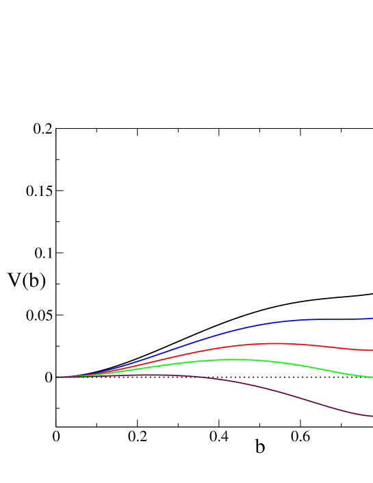
The condition $n_{1}=0$ (11), is equivalent to $V^{\prime}(b)=0$. Thus, if $V(b)$ has a single minimum in $b=0$, the solution space is not clustered, while if there is another minimum at $b\neq 0$, there are clusters. Moreover, the condition for satisfiability (12), is that at the secondary minimum $V(b)\geq 0$. Examples are given in figure 2.

The sat/unsat surface $\Sigma_{s}$, that separates the sat and the unsat phase, is defined by the condition:

$$\Sigma_{s}\equiv\{c_{j}:V(b)=0\ \mbox{and}\ V^{\prime}(b)=0\ \mbox{admit a solution}\ b>0\}\ .$$ (14)

The clustering surface $\Sigma_{d}$, that separates the clustered and unclustered regions, is defined similarly by

$$\Sigma_{d}\equiv\{c_{j}:V^{\prime}(b)=0\ \mbox{and}\ V^{\prime\prime}(b)=0\ \mbox{admit a solution}\ b>0\}\ .$$ (15)

The equations above have to be interpreted as coupled equations for $(b,c_{j})$; therefore $\Sigma_{s},\Sigma_{d}$ have dimension $k-2$ and are surfaces in the space $\{c_{j}\}_{j=2,\cdots,k}$ of dimension $k-1$. Note that in (14) and (15), one must always choose the largest solution for $b$, to which we will refer as $b_{s}$ and $b_{d}$, respectively.

In addition to the previous sets, in the following a special role will be played by the condition $2c_{2}=1$, or equivalently $V^{\prime\prime}(0)=0$, that defines the contradiction surface $\Sigma_{q}$:

$$\Sigma_{q}\equiv\{c_{j}:V^{\prime\prime}(0)=0\}\ .$$ (16)

The surface $\Sigma_{q}$ is simply a hyperplane of dimension $k-2$.

3.4 The phase diagram

Figure 1: (Left) Schematic phase diagram of $k$$=$4-UE-CSP. The full (black) curve is the surface $\Sigma_{d}$, the dot-dashed (red) surface is $\Sigma_{s}$. The two surfaces meet along a portion of the line $\Sigma_{crit}$, defined by $c_{2}=1/2$ and $c_{3}=1/6$ and represented as a dashed (blue) line. (Right, top and bottom) The sections of $\Sigma_{d}$ (full, black) and of $\Sigma_{s}$ (dot-dashed, red), at fixed $c_{2}$ (= 0, 0.1, 0.2, 0.3, 0.4, 0.5 from top to bottom) as a function of $c_{3}$ on the top panel, and at fixed $c_{4}$ (= 0, 0.1, 0.2, 0.3, 0.4, 0.5, 0.6, 0.7 from top to bottom) as a function of $c_{2}$ in the bottom one. The lines corresponding to $c_{4}=0$ also represent the phase diagram of 3-UE-CSP.

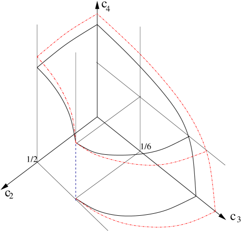
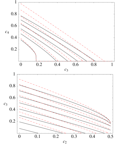
We draw a phase diagram in the space of the $c_{j}$ by representing surfaces $\Sigma_{s},\Sigma_{d},\Sigma_{q}$. We focus on the region $c_{j}\in[0,1]$ for $j=3,\ldots,k$ and $c_{2}\in[0,1/2]$. Indeed, if one of the $c_{j}>1$, the system is surely in the unsat phase [7] while if $c_{2}>1/2$ the algorithm discussed above find a contradiction with very high probability.

Examples of the phase diagram are in figure 1 for $k=3$ and $k=4$. There are some special “lines” (i.e. intersections of surfaces) on which we will concentrate.

1. Recall that $\Sigma_{q}$ is defined by $V^{\prime\prime}(0)=0$ and note that $V^{\prime}(0)=0$ for all $b$, $c_{j}$. Thus, on $\Sigma_{q}$, the point $b=0$ is a solution of both equations (14) and (15). The surfaces $\Sigma_{s},\Sigma_{d}$ are defined by the existence of solutions with $b>0$, but they might intersect $\Sigma_{q}$ if for some values of $\{c_{j}\}$ the solution with $b>0$ merges with the solution $b=0$. This happen when $V^{\prime\prime\prime}(0)=0$, as this is the limiting case in which a saddle at $b=b_{d}>0$ and a secondary minimum at $b=b_{s}>0$ can merge for $b_{d},b_{s}\rightarrow 0$. The condition $V^{\prime\prime\prime}(0)=0$ is equivalent to $c_{3}=1/6$, and this defines the $k-3$-dimensional surface

   $$\Sigma_{crit}\equiv\{c_{j}:c_{2}=1/2,c_{3}=1/6\}\ ,$$ (17)

   to which we will refer as critical surface. It is easy to see that the three surfaces $\Sigma_{s},\Sigma_{d},\Sigma_{q}$ are tangent to each other on the region of the critical surface where they intersect. To show that one must consider a displacement $c_{3}=1/6+\varepsilon$ and show that (15), (14) admit a solution with $b_{s},b_{d}\sim\varepsilon$ if $c_{2}-1/2\sim\varepsilon^{2}$. We say that in this case the phase transitions are of second order because the order parameter $b$ vanishes continuously at the transition.

2. There is no a priori reason for which the three surfaces must cross at $\Sigma_{crit}$. In fact, the solutions at $b>0$ might also disappear discontinuously, like in figure 2, and the surfaces $\Sigma_{s}$ and $\Sigma_{d}$ can intersect the surface $\Sigma_{q}$ in regions different from $\Sigma_{crit}$. This does not happen for $k=3$ but happens for $k=4$ for large $c_{4}$, see figure 1. In this case the transition is called first order because the order parameter jumps at the transition.

The generic phase diagram for all $k$ has the shape of the one for $k=4$ which we report in figure 1, left panel.

4 Search Trajectories in the Space of Formulas

The heuristics we defined in section 2 enjoy the property that, after any number of steps of the algorithm, the reduced formula is uniformly distributed over the set of remaining $N-T$ variables conditioned to the numbers $C_{j}(T)$ of clauses of length $j$ ($=2,...,k$) [8, 9]. This statistical property, combined with the concentration phenomenon taking place in the large $N$ limit, allows us to study the evolution of the average clauses densities $c_{j}(t)=C_{j}(T)/N$ on the time scale $t=T/N$ (fraction of assigned variables), which defines a trajectory in the $c_{j}$’s space. Note that these $c_{j}(t)$ are defined with respect to $N$, therefore the actual clause density for the reduced system of $N-T$ variables are $\widetilde{c}_{j}(t)=c_{j}(t)/(1-t)$. The trajectory of the $\widetilde{c}_{j}(t)$ moves in the $c_{j}$ space of the previous section.

Initially we have $c_{j}(0)=\alpha\;\delta_{jk}$, i.e. the evolution starts on the $c_{k}$ axis at $c_{k}=\alpha$. The evolution equation for the densities take the form of first order differential equations,

$$\dot{c}_{j}=\frac{(j+1)c_{j+1}-jc_{j}}{1-t}-\rho_{j}(t)\ .$$ (18)

The interpretation of the equations above is the following. Let us consider an interval $[t,t+dt]$ of continuous time that corresponds to $\Delta T\sim Ndt$ time steps of the algorithm. The first term on the r.h.s. arises from the decrease by one of the length of the clauses that contained the variable just assigned by the algorithms during this interval. The second term corresponds to an additional loss of clauses which is present when the variable is selected from a clause of length $j$: as the heuristics explicitly chooses an equation (and a variable therein) of length $j$ with probability $p_{j}$ (see section 2), this equation will be reduced irrespectively of the number of other occurrences of the variable. Hence $\rho_{j}(t)$ is given, for $j\geq 1$, by

$$\rho_{j}(t)=\lim_{\Delta T\rightarrow\infty}\lim_{N\rightarrow\infty}\frac{1}{\Delta T}\sum_{T=tN}^{tN+\Delta T-1}\left(p_{j}-p_{j+1}\right)\equiv\left\langle p_{j}-p_{j+1}\right\rangle\ ,$$ (19)

where both $p_{j},p_{j+1}$ depend on their arguments (numbers of clauses) and $\left\langle\bullet\right\rangle$ represents the average over $\Delta T$ defined in (19). Here $p_{k+1}\equiv 0$. Note that the case $j=1$ is special as all clauses of length one that are produced are immediately eliminated. On average

$$\rho_{1}\equiv\frac{2c_{2}}{1-t}$$ (20)

clauses of length 2 become of length 1 and are then eliminated by unit propagation. The total fraction of eliminated clauses is

$$\dot{\gamma}(t)\equiv-\sum_{j=2}^{k}\dot{c}_{j}(t)=\frac{2c_{2}(t)}{1-t}+\sum_{j=2}^{k}\rho_{j}(t)=\sum_{j=1}^{k}\rho_{j}(t)\leq 1\ ,$$ (21)

where the last inequality follows from (19). As only clauses of length one are eliminated, the violation of (21) can only happen if too many such clauses are generated. This corresponds to $\rho_{1}\rightarrow 1^{-}$; in this case a contradiction occurs with high probability and the algorithm stops with the ‘Don’t know’ output. When $\rho_{1}\rightarrow 1^{-}$, the algorithm makes only unit propagations and $\rho_{j}\rightarrow 0^{+}$ for all $j\geq 2$. For this reason we called the plane $\rho_{1}=1$, i.e. $\widetilde{c}_{2}=1/2$, contradiction surface.

4.1 Unit Clause (UC)

In the UC heuristic variables are chosen at random when there is no unit clause. Hence $\rho_{j}=0$ for $j=2,\cdots,k$. The solution to (18) is $c_{j}(t)=\alpha{k\choose j}(1-t)^{j}t^{k-j}$. The algorithm will generate a contradiction with high probability (w.h.p.) if the average number of unit clauses starts to build-up, i.e. if $2c_{2}(t)/(1-t)\geq 1$. This gives an equation for the value of $\alpha$ at which the probability that the algorithm finds a solution vanishes: for $k=3$, $\alpha_{a}^{\mathrm{(UC)}}=2/3$.

4.2 Generalized Unit Clause (GUC)

In the GUC heuristic the algorithm always fixes a variable appearing in the shortest clauses. In the continuum limit $c_{j}=0$ for $j$ smaller than a given value; therefore we define

$$j^{*}(t)=\min\{j:c_{j}(t)>0\}\ ,$$ (22)

the minimal length of clauses with positive densities. We also define

$$t^{*}(j)=\min[t:c_{j-1}(t)>0]$$ (23)

the time at which $j^{*}$ jumps down from $j$ to $j-1$. Essentially, the algorithm picks one clause of length $j^{*}$ and assigns successively all the variables in this clause until the clause disappears. But in doing so, other clauses of length $j<j^{*}$ are generated and have to be eliminated to recover the situation in which $C_{j}=0$ for all $j<j^{*}$; for this reason $\rho_{j^{*}}$ is not given exactly by $1/j^{*}$. When the number of generated clauses is so high that the algorithm is unable to remove them, $c_{j^{*}-1}$ becomes different from 0 and $j^{*}$ jumps down by 1. The resulting motion equations for the clause densities are, for $j\geq j^{*}(t)$:

$$\dot{c}_{j}(t)=\frac{(j+1)c_{j+1}(t)-jc_{j}(t)}{1-t}-\delta_{j,j^{*}(t)}\left(\frac{1}{j}-\frac{(j-1)c_{j}(t)}{1-t}\right)\ .$$ (24)

The transition times $t^{*}$ are given by

$$\frac{c_{j}(t^{*}(j))}{1-t}=\frac{1}{j(j-1)}\ ,$$ (25)

where the algorithm is no more able to remove the clauses of length $j^{*}$ because too many clauses of length $j^{*}-1$ are being generated by propagations.

Comparing with (18) above, we observe that in the interval $t\in[t^{*}(j+1),t^{*}(j)]$, where $j^{*}=j$, only two $\rho_{j}$ are different from 0:

$$\rho_{j^{*}}=\frac{1}{j^{*}}-\frac{(j^{*}-1)c_{j^{*}}(t)}{1-t}\ ,\ \ \ \ \rho_{j^{*}-1}=\frac{j^{*}c_{j^{*}}(t)}{1-t}\ ,$$ (26)

the first representing clauses of length $j^{*}$ which are directly eliminated, the second representing the clauses of length $j^{*}-1$ that are produced and subsequently eliminated in the process. In this interval of time, the ratio $c_{j^{*}}(t)/(1-t)$ increases from 0 to $1/j^{*}/(j^{*}-1)$ from condition (25). Then

$$\frac{1}{j^{*}(t)}\leq\dot{\gamma}(t)=(\rho_{j^{*}}+\rho_{j^{*}-1})\leq\frac{1}{j^{*}(t)-1}\ ,$$ (27)

which is consistent with (but stronger than) (21) above.

5 Analysis of the “dynamic” phase diagram

Figure 2: An example of the potential $V(b;t,\alpha)$ plotted (from top to bottom) at times $t=\{0,t_{d}=0.02957,0.07327,t_{s}=0.11697,0.20642\}$ during the evolution of a $(3,d)$-UE-CSP formula with $\alpha=0.8$ under the UC heuristic. In the unclustered region it is a convex function of $b$ with a global minimum in $b=0$. On the clustering line $t_{d}$ it first develops a secondary minimum. On the sat/unsat line the value of $V$ at the secondary minimum becomes equal to 0.

Consider now a given heuristic, and a generic $(k,d)$-UE-CSP formula specified by its clause-to-variable ratio $\alpha$. The formula, in the $c_{j}$ space, starts on the axis $c_{k}$ at $c_{k}=\alpha$. The evolution of the formula under the action of the algorithm is represented by a trajectory $\{c_{j}(t,\alpha)\}_{j=2,\cdots,k}$ or equivalently by $G(b;t,\alpha)=\sum_{j=2}^{k}b^{j}c_{j}(t,\alpha)$, that depends on $\alpha$ through the initial condition $G(b;0,\alpha)=\alpha b^{k}$. We define a potential $V(b;t,\alpha)$ by replacing in (13) $G(b)\rightarrow G(b;t,\alpha)/(1-t)$; the normalization $(1-t)$ is due to the fact that the $c_{j}=C_{j}/N$ are divided by $N$ instead of $N-T$.

We follow the evolution of the formula by looking at the times at which the trajectory starting at $c_{k}=\alpha$ at time $0$ crosses the surfaces $\Sigma_{s},\Sigma_{d},\Sigma_{q}$ defined in section 3.3, which we call $t_{s}(\alpha),t_{d}(\alpha),t_{q}(\alpha)$ respectively. As an example, in figure 2 we report the potential at different times during the evolution of a formula according to the UC heuristic for $\alpha>\alpha_{a}^{(UC)}$.

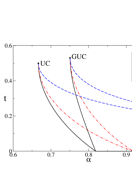
We draw a “dynamic phase diagram” by representing in the $(t,\alpha)$ plane the lines separating the unclustered, clustered, unsat and contradiction phases, which we call $\alpha_{d}(t),\alpha_{s}(t),\alpha_{q}(t)$ and are just the inverse of the times defined above. Examples in the case of the UC and GUC heuristics are given in figure 3.

From the general properties of the function $V(b;t,\alpha)$ we can deduce a number of properties of the lines $\alpha_{d}(t),\alpha_{s}(t),\alpha_{q}(t)$. We will show that the three lines intersect at a “critical point” $(t_{a},\alpha_{a})$, located at $\alpha_{a}\leq\alpha_{d}$, under the more general conditions. This implies that the algorithm stops working at the value $\alpha_{a}\leq\alpha_{d}$, which is our central result: Poissonian search algorithm cannot find a solution in polynomial time in the clustered region.

5.1 Equations for the transition lines

Figure 3: (Left) Phase boundary lines in the $(t,\alpha)$ plane for the UC and GUC heuristics for $k=3$. The three lines meet at the critical point $(t_{a},\alpha_{a})$ at which the algorithm is no more able to find a solution (black dot). (Right) The generic shape of the clustering and of the sat/unsat lines. The possibility of a maximum cannot be excluded, but in any case $t$ must be a single-valued function of $\alpha$, meaning that if the algorithm enters the cluster (or unsat) phase it cannot escape at later times.

The generating function $G(b;t,\alpha)$ satisfy an evolution equation which is easily derived from (18):

$$\dot{G}(b;t,\alpha) = \frac{1-b}{1-t}G^{\prime}(b;t,\alpha)-F(b;t,\alpha)\ ,$$ (28)

$$F(b;t,\alpha) \equiv \frac{2c_{2}(t)}{1-t}b+\sum_{j=2}^{k}\rho_{j}(t)b^{j}=\sum_{j=1}^{k}\rho_{j}(t)b^{j}\ .$$ (29)

Performing the total derivative with respect to $t$ of the first condition ($V^{\prime}=0$) in (15) for $(\alpha_{d},b_{d})$ and using the second condition, $V^{\prime\prime}=0$, we have

$$\frac{\partial V^{\prime}}{\partial\alpha}\frac{d\alpha_{d}}{dt}+\dot{V}^{\prime}=0\ \ \ \ \Rightarrow\ \ \ \ \frac{d\alpha_{d}}{dt}=-\frac{\dot{V}^{\prime}(b_{d};t,\alpha_{d})}{\frac{\partial V^{\prime}}{\partial\alpha}(b_{d};t,\alpha_{d})}\ .$$ (30)

Using the definition (13) we have

$$\dot{V}^{\prime}(b;t,\alpha) = -\frac{1}{1-t}\left[\dot{G}^{\prime}(b;t,\alpha)+\frac{G^{\prime}(b;t,\alpha)}{1-t}\right]\ ,$$ (31)

$$\frac{\partial V^{\prime}}{\partial\alpha} = -\frac{1}{1-t}\frac{\partial G^{\prime}}{\partial\alpha}=-\frac{1}{1-t}\sum_{j\geq 2}jb^{j-1}\frac{\partial c_{j}(t,\alpha)}{\partial\alpha}\ .$$ (32)

Then

$$\frac{d\alpha_{d}}{dt}=-\left.\frac{\dot{G}^{\prime}(b;t,\alpha)+\frac{G^{\prime}(b;t,\alpha)}{1-t}}{\partial_{\alpha}G^{\prime}(b;t,\alpha)}\right|_{\alpha=\alpha_{d}(t),b=b_{d}(t)}\ .$$ (33)

Using (28) and differentiating with respect to $b$ we have

$$\dot{G}^{\prime}(b;t,\alpha)+\frac{G^{\prime}(b;t,\alpha)}{1-t}=\frac{1-b}{1-t}G^{\prime\prime}(b;t,\alpha)-F^{\prime}(b;t,\alpha)\ .$$ (34)

Now using $V^{\prime\prime}(b;t,\alpha)=-\frac{G^{\prime\prime}(b;t,\alpha)}{1-t}+\frac{1}{1-b}$ and $V^{\prime\prime}(b_{d},t)=0$ we have $\frac{1-b}{1-t}G^{\prime\prime}(b;t,\alpha)=1$ for $b=b_{d}$ and finally we get

$$\frac{d\alpha_{d}}{dt}=-\left.\frac{1-F^{\prime}(b;t,\alpha)}{\partial_{\alpha}G^{\prime}(b;t,\alpha)}\right|_{\alpha=\alpha_{d}(t),b=b_{d}(t)}\ .$$ (35)

A very similar reasoning leads to the following equation for the sat/unsat line:

$$\frac{d\alpha_{s}}{dt}=-\left.\frac{b-F(b;t,\alpha)}{\partial_{\alpha}G(b;t,\alpha)}\right|_{\alpha=\alpha_{s}(t),b=b_{s}(t)}\ .$$ (36)

The equation for the contradiction line is easily derived from its definition $\widetilde{c}_{2}(t,\alpha)=\frac{c_{2}(t,\alpha)}{1-t}=\frac{1}{2}$, which immediately gives

$$\frac{d\alpha_{q}}{dt}=-\left.\frac{1+2\dot{c}_{2}(t,\alpha)}{2\partial_{\alpha}c_{2}(t,\alpha)}\right|_{\alpha=\alpha_{q}(t)}\ .$$ (37)

5.2 General properties of the transition lines

We wish to show that the transition lines $t_{d}(\alpha)$,$t_{s}(\alpha)$ and $t_{q}(\alpha)$ in the $(\alpha,t)$ plane are single-valued functions of $\alpha$, and that they meet in a point $(\alpha_{a},t_{a})$ where they have infinite slope and are therefore tangent to each other; the value $\alpha_{a}$ correspond to a trajectory which is tangent to the crytical surface $\Sigma_{crit}$.

Our argument goes as follows:

1. We defined $\alpha_{a}$ as the value of $\alpha$ for which the probability of finding a solution for the chosen heuristic vanishes. Then the trajectory corresponding to any $\alpha>\alpha_{a}$ must cross the contradiction surface, while the trajectory corresponding to any $\alpha<\alpha_{a}$ must not cross it, so that the trajectory corresponding to $\alpha_{a}$ must be tangent to the contradiction surface $\Sigma_{q}$. The latter trajectory is tangent to $\Sigma_{q}$ when $\widetilde{c}_{2}(t)=1/2$, $\frac{d}{dt}\widetilde{c}_{2}(t)=0$; the solution to these conditions gives $t_{a}$ and $\alpha_{a}$.
   Moreover, $\widetilde{c}_{2}(t)=1/2$ implies that $\rho_{1}=1$ which then implies $\rho_{j}=0$ for all $j\geq 2$, as already discussed. Then we have

   $$\frac{d}{dt}\widetilde{c}_{2}(t)=\frac{d}{dt}\frac{2c_{2}(t)}{1-t}=\frac{2\dot{c}_{2}(t)}{1-t}+\frac{2c_{2}(t)}{(1-t)^{2}}=0\ \ \ \Rightarrow\ \ \ \dot{c}_{2}(t)=-\frac{c_{2}(t)}{1-t}=-\frac{1}{2}\ ,$$ (38)

   which, together with the equations of motion (18) and $\rho_{2}=0$ gives

   $$-\frac{c_{2}(t)}{1-t}=\frac{dc_{2}(t)}{dt}=\frac{3c_{3}(t)-2c_{2}(t)}{1-t}\ \ \ \Rightarrow\ \ \ \widetilde{c}_{3}(t)=\frac{c_{3}(t)}{1-t}=\frac{1}{3}\frac{c_{2}(t)}{1-t}=\frac{1}{6}\ .$$ (39)

   Therefore the point where the trajectory for $\alpha=\alpha_{a}$ is tangent to the contradiction surface belongs to the critical surface $\Sigma_{crit}$. From equation (37) it is clear that since $\dot{c}_{2}=-1/2$, the function $t_{q}(\alpha)$ has infinite slope in $(t_{a},\alpha_{a})$, as in figure 3.

2. Next we show that the numerators of the fractions appearing in $\dot{\alpha}_{d}(t)$ and $\dot{\alpha}_{s}(t)$ are strictly positive if $t<t_{q}(\alpha)$, i.e. in before a contradiction is found. Using the definition (19) we can write:

   $$F(b;t,\alpha) = \sum_{j=1}^{k}\rho_{j}(t)b^{j}=b\left[\left\langle p_{1}\right\rangle+\sum_{j=2}^{k}b^{j-2}(b-1)\left\langle p_{j}\right\rangle\right]\ ,$$ (40)

   $$F^{\prime}(b;t,\alpha) = \sum_{j=1}^{k}j\rho_{j}(t)b^{j-1}=\left\langle p_{1}\right\rangle+\sum_{j=2}^{k}b^{j-2}\left[1-j(1-b)\right]\left\langle p_{j}\right\rangle\,.$$

   The coefficients in front of $\left\langle p_{j}\right\rangle\geq 0$ in the sums above are always smaller than 1, independently of $j$, so that

   $$F(b;t,\alpha) \leq b\left[\left\langle p_{1}\right\rangle+\sum_{j=2}^{k}\left\langle p_{j}\right\rangle\right]\leq b\ ,$$ (41)

   $$F^{\prime}(b;t,\alpha) \leq \left\langle p_{1}\right\rangle+\sum_{j=2}^{k}\left\langle p_{j}\right\rangle\leq 1\,.$$ (42)

   The functions $F(b;t,\alpha)$ and $F^{\prime}(b;t,\alpha)$ are to be computed in $b=b_{s}(t,\alpha)$ or $b=b_{d}(t,\alpha)$ in equations (35) and (36). Both $b_{s}$ and $b_{d}$ are strictly smaller than $1$ for all $(t,\alpha)$, as one can directly show from their definitions because $V^{\prime}(b\rightarrow 1)\rightarrow\infty$. Then the coefficients in the sums in (40) are strictly smaller than $1$, and the only solution to $F=b$ or $F^{\prime}=1$ is $\left\langle p_{j}\right\rangle=\delta_{1j}$, which happens only on the contradiction line.

3. The denominators in equations (35), (36) are surely positive at $t=0$, as $G(b;0,\alpha)=\alpha b^{k}$ independently of the heuristic. If they remain positive at all times, then $\dot{\alpha}_{d}(t),\dot{\alpha}_{s}(t)\leq 0$ at all times, or equivalently $\frac{dt_{d}}{d\alpha},\frac{dt_{s}}{d\alpha}\leq 0$ at all $\alpha$, so that $t_{d},t_{s}$ always increase on decreasing $\alpha$.
   The other possibility is that the denominator in (35) crosses zero and become negative, leading to a maximum in $t_{d}(\alpha)$, which will then decrease on decreasing $\alpha$. Possibly the denominators can vanish again, giving rise to a sequence of maxima and minima, see right panel of figure 3.
   What is important is that the numerator is always strictly positive, and as a consequence $t_{d}(\alpha)$ or $t_{s}(\alpha)$ are single-valued functions of $\alpha$. In fact, for $t_{d}(\alpha)$ or $t_{s}(\alpha)$ to be multiple-valued functions of $\alpha$, at some point their slope must become infinite, which is excluded by the analysis above.

4. The statement above, that $t_{d}(\alpha)$ and $t_{s}(\alpha)$ are single valued functions of $\alpha$, implies that if a trajectory enters the clustered or unsat phase, it cannot exit from it. This is enough to show that $\alpha_{a}\leq\alpha_{d}$; in fact, the trajectory for $\alpha=\alpha_{a}$ cannot start inside the clustered phase, as it would not be able to escape and reach the origin, which is required to find a solution.

5. In general the function $\widetilde{c}_{2}(t)$ increases until it reaches a maximum and then decreases to 0. For $\alpha=\alpha_{a}$ the value at the maximum is $\widetilde{c}_{2}=1/2$. For $\alpha>\alpha_{a}$, the value at the maximum is $\widetilde{c}_{2}>1/2$, therefore the contradiction $\widetilde{c}_{2}=1/2$ is reached before the maximum, when $\widetilde{c}_{2}$ is still increasing. Then $\frac{d}{dt}\widetilde{c}_{2}>0$ at the contradiction point. Performing a simple computation similar to equations (38), (39), one can show that the trajectories for $\alpha>\alpha_{a}$ meet the contradiction surface at $\widetilde{c}_{3}>1/6$. Notice then that, as it is evident in figure 1, the trajectories corresponding to $\alpha>\alpha_{a}$ must enter first the clustered and then the unsat phases in order to reach the contradiction surface, therefore for $\alpha<\alpha_{a}$ one has $t_{d}(\alpha)<t_{s}(\alpha)<t_{q}(\alpha)$. On the contrary the trajectories corresponding to $\alpha<\alpha_{a}$ must stay away from the clustering and sat/unsat surfaces, otherwise they could not exit and should meet the contradiction surface: therefore for any $\alpha<\alpha_{a}$, $t_{d}(\alpha)$ and $t_{s}(\alpha)$ do not exist. For $\alpha\rightarrow\alpha_{a}^{+}$, as the surfaces $\Sigma_{d},\Sigma_{s},\Sigma_{q}$ are tangent in $\Sigma_{crit}$, one has $t_{d}(\alpha_{a})=t_{s}(\alpha_{a})=t_{q}(\alpha_{a})=t_{a}$ and the three curves have infinite slope as all the numerators in equations (35), (36), (37) vanish on the contradiction surface. This is indeed what is observed in figure 3 for the UC and GUC heuristics, and this argument confirms that this is the generic behavior for all the heuristics in the class considered here.

This structure is particularly evident for UC, where

$$G^{\mathrm{(UC)}}(b;t,\alpha)=\alpha[1-(1-b)(1-t)]^{k}-\alpha t^{k-1}[kb(1-t)+t]\ .$$ (43)

From (43) it is straightforward to check that $\partial_{\alpha}G(b;t,\alpha)>0$, $\partial_{\alpha}G^{\prime}(b;t,\alpha)>0$, if $b>0$. Then, as $F(b;t,\alpha)=\frac{2bc_{2}(t)}{1-t}$ for UC, both $\dot{\alpha}_{d}(t)$ and $\dot{\alpha}_{s}(t)$ are proportional to $\frac{2c_{2}(t)}{1-t}-1$. This means that $\alpha_{s}$,$\alpha_{d}$ are decreasing functions of $t$ below the contradiction line.

The conclusion is that for a generic Poissonian heuristic, the three lines cross at a critical point $(t_{a},\alpha_{a})$ which depends on the heuristic. Above $\alpha_{a}$ the heuristic will cross all the lines and find a contradiction. From the properties of the dynamical line, we have that generically $\alpha_{a}\leq\alpha_{d}$, that is no Poissonian search heuristic can find a solution in polynomial time above $\alpha_{d}$, as stated at the beginning of this section. The natural question is then if there exists an heuristic that saturates the bound, i.e. such that $\alpha_{a}=\alpha_{d}$. From the discussion above it is clear that this is possible only if $\dot{\alpha}_{d}(t)\equiv 0$, i.e. the dynamical line in the $(t,\alpha)$ plane is a straight vertical line, which is possible only if the numerator in (35) is identically vanishing.

5.3 Optimality of GUC

It is quite easy to see that GUC is the heuristic that locally optimizes the numerator in (35). Indeed, from the definition $F^{\prime}(b;t,\alpha)=\sum_{j=1}^{k}jb^{j-1}\rho_{j}$ and the bound $F^{\prime}(1,t)\leq 1$, it is clear that $F^{\prime}(b;t,\alpha)$ is maximized by maximizing $\rho_{j}$ for the smallest possible $j$, i.e. by picking clauses from the shortest possible ones, that is GUC. Unfortunately a general proof of the optimality of GUC for finite $k$ seems difficult, because one should prove that GUC optimizes globally the clustering line, and also control the denominator in (35). In this section we will show that for $k\rightarrow\infty$, GUC is optimal in the sense that $\dot{\alpha}_{d}\equiv 0$ and $\alpha_{d}=\alpha_{a}$ at leading order in $k$.

From the definition $\gamma(t)=-\sum_{j=2}^{k}c_{j}(t)$ and integrating over time the bound (27), we have for GUC:

$$\alpha-\int_{0}^{t}\frac{dt^{\prime}}{j^{*}(t^{\prime})-1}\leq-\gamma(t)\leq\alpha-\int_{0}^{t}\frac{dt^{\prime}}{j^{*}(t^{\prime})}\ .$$ (44)

or, equivalently,

$$\alpha-\sum_{j}\frac{t^{*}(j)-t^{*}(j+1)}{j-1}\leq-\gamma(t)\leq\alpha-\sum_{j}\frac{t^{*}(j)-t^{*}(j+1)}{j}\ .$$ (45)

where the sums are limited to the values of $j$ that are reached during the search. In the large $k$ limit, provided the hypothesis

$$t^{*}(j)-t^{*}(j+1)=\frac{1}{k}+o(1/k)$$ (46)

holds for most $j$, we obtain

$$-\gamma(t)\simeq\alpha-\frac{1}{k}\sum_{j^{*}(t)}^{k}\frac{1}{j}\ .$$ (47)

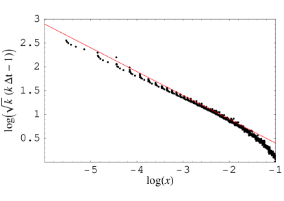
The hypothesis (46) is well supported by numerical data, as shown in figure 4. As the sum of the inverse of the first $k$ integers is equivalent to $\log k$ (harmonic number) we see that the minimal value of $j^{*}$ over $t$ is much larger than 2 if $\alpha$ is much smaller than $\log k/k$. Therefore

$$\alpha_{a}\geq\frac{\log k}{k}\ .$$ (48)

The r.h.s. of the above inequality coincides with the asymptotic scaling of the clustering critical ratio (section 3.2). Since the results of the previous section require that $\alpha_{a}\leq\alpha_{d}$, we obtain that $\alpha_{a}^{\mathrm{(}GUC)}=\alpha_{d}\simeq\log k/k$ at the leading order in $k\rightarrow\infty$. As a comparison, it is easy to see that for UC the threshold for large $k$ is $\alpha_{a}^{\mathrm{(}UC)}\simeq e/k$, which is therefore much lower than the threshold for GUC.

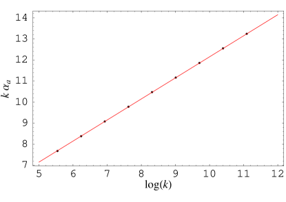
These arguments are supported by numerical simulations that we performed up to $k=2^{16}$, in which the equations of motion (24) are integrated as finite differences equations for all values of $j$ (see figure 4). The numerical investigation confirms that $k\alpha_{a}^{\mathrm{(}GUC)}$ is very well fitted by $\log k+2.15$ for $k$ in the range $2^{8}\div 2^{16}$. Moreover, a finite size scaling analysis (with respect to $k$) of the data shown in figure 4 shows that

$$k[t^{*}(j)-t^{*}(j+1)]=1+k^{\nu}\times f(j/k)$$ (49)

where $f(x)$ is a function independent on $k$ which behaves as $x^{-\mu}$ for $x$ close to 0. From the numerical data, it appears that $\nu=\mu=0.5$, which confirms that the first correction to the leading term $\log k/k$ is of order $1/k$.

Figure 4: Finite size scaling results for GUC at large $k$. Top Left Each curve shows the values of $k[t^{*}(j)-t^{*}(j+1)]$ as a function of $j/k$ for $k=2^{8},2^{9},\dots,2^{16}$ (from the farthest to the closest curve to 1), and was obtained by integrating the equations of motion (24) by finite differences. For each $k$, the value of $\alpha$ used is $\alpha_{a}^{\mathrm{GUC}}(k)$, determined as the value of $\alpha$ for which the maximum reached by $2c_{2}(t)/(1-t)$ is 1. Top Right Data points of $\alpha_{a}^{\mathrm{GUC}}(k)$ versus $\log k/k+2.15/k$ (full red line). Bottom left The same data as above, plotted as $\{k\times[t^{*}(j)-t^{*}(j+1)]\}\times k^{1/2}$. The curves “collapse”, showing $f(x)$ and confirming the value of $\nu=1/2$. Bottom right By plotting the same curves on logarithmic scale it is easily seen that for $x$ close to 0 $f(x)\simeq x^{-\mu}$ with $\mu=1/2$, corresponding to the slope of the full red line.

6 Conclusions

One of the main results of this paper, that is, that linear-time search heuristic are not able to solve instances in the clustered phase of UE-CSP problems should be interpreted with care. In XORSAT-like models the clustering transition coincide with the emergence of strong correlations between variables in solutions, while the two phenomena generally define two distinct critical ratios for other random decision problems [15, 16]. From an intuitive point of view it is expected that the performances of search heuristics are affected by correlations between variables rather than the clustering of solutions. Indeed, as the search algorithms investigated here do not allow for backtracking or corrections of wrongly assigned variables, very strong correlations between $O(N)$ variables (recall that the backbone includes $O(N)$ variables in the clustered phase) are likely to result in $e^{-O(N)}$ probabilities of success for the algorithm.

Extending the present work to the random Satisfiability ($k$-SAT) problem would be interesting from this point of view, because even if the clustering and freezing transition coincide at leading order for $k\rightarrow\infty$ [3], their finite $k$ values are different in this case. Moreover, in some similar problems ($k$-COL [17] and 1-in-$k$-SAT [18]) it has been proven that search algorithms similar to the ones investigated here are efficient beyond the point where the replica-symmetry-breaking solution is stable. Therefore these algorithms might beat the clustering threshold in these problems. Note however that in these cases the transition is continuous, so that the structure of the clusters is expected to be very different from the one of XORSAT.

In addition, while the Generalized Unit Clause heuristic is here shown to be optimal for the $k$-XORSAT problem and to saturate the clustering ratio when $k\rightarrow\infty$, it is certainly not the case of the $k$-SAT problem. Determining a provably optimal search heuristic for this problem remains an open problem.

References

- [1] Mézard M, Parisi G and Virasoro M A 1987 Spin glass theory and beyond (Singapore: World Scientific)
- [2] Biroli G, Monasson R and Weigt M 2000 Eur. Phys. J. B 14 551
- [3] Krzakala F, Montanari A, Ricci-Tersenghi F, Semerjian G and Zdeborová L 2007 Proc. Natl. Acad. Sci. USA 104 10318
- [4] Montanari A and Semerjian G 2006 J. Stat. Phys. 124 103
- [5] Monasson R 2007 Introduction to Phase Transitions in Random Optimization Problems, Lecture Notes of the Les Houches Summer School on Complex Systems, Elsevier
- [6] Krzakala F and Kurchan J 2007 Phys. Rev. E 76 021122
- [7] Connamacher H 2004 A Random Constraint Satisfaction Problem That Seems Hard for DPLL, Proceedings of the Seventh International Conference on Theory and Applications of Satisfiability Testing
-
[8]
Chao M T and Franco J 1990
Information Science 51 289
Chao M T and Franco J 1986 SIAM Journal on Computing 15 1106 - [9] Achlioptas D 2001 Theor. Comp. Sci. 265 159
- [10] Achlioptas D, Beame P and Molloy M 2004 J. Comput. Syst. Sci. 68 238
- [11] Dubois O and Mandler J 2002 The 3-XORSAT Threshold, Proceedings of the 43rd Symposium on Foundations of Computer Science
- [12] Mézard M, Ricci-Tersenghi F and Zecchina R, 2003 J. Stat. Phys. 111 505
- [13] Cocco S, Dubois O, Mandler J and Monasson R 2003 Phys. Rev. Lett. 90 047205
- [14] Weigt M 2002 Eur. Phys. J. B 28 369
- [15] Semerjian G 2007 On the freezing of variables in random constraint satisfaction problems Preprint arXiv:cond-mat/07052147 (J.Stat.Phys. in press)
- [16] Krzakala F and Zdeborová L 2007 Phys. Rev. E 76 031131
- [17] Achlioptas D and Moore C 2003 J. Comput. Syst. Sci. 67 441
- [18] Raymond J, Sportiello A and Zdeborová L 2007 Phys. Rev. E 76 011101