On the relation between the Schmidt and Kennicutt-Schmidt star formation laws and its implications for numerical simulations

Abstract

When averaged over large scales, star formation in galaxies is observed to follow the empirical Kennicutt-Schmidt (KS) law for surface densities above a constant threshold. While the observed law involves surface densities, theoretical models and simulations generally work with volume density laws (i.e. Schmidt laws). We derive analytic relations between star formation laws expressed in terms of surface densities, volume densities, and pressures and we show how these relations depend on parameters such as the effective equation of state of the multiphase interstellar medium. Our analytic relations enable us to implement observed surface density laws into simulations. Because the parameters of our prescription for star formation are observables, we are not free to tune them to match the observations. We test our theoretical framework using high-resolution simulations of isolated disc galaxies that assume an effective equation of state for the multiphase interstellar medium. We are able to reproduce the star formation threshold and both the slope and the normalisation of arbitrary input KS laws without tuning any parameters and with very little scatter, even for unstable galaxies and even if we use poor numerical resolution. Moreover, we can do so for arbitrary effective equations of state. Our prescription therefore enables simulations of galaxies to bypass our current inability to simulate the formation of stars. On the other hand, the fact that we can reproduce arbitrary input thresholds and KS laws, rather than just the particular ones picked out by nature, indicates that simulations that lack the physics and/or resolution to simulate the multiphase interstellar medium can only provide limited insight into the origin of the observed star formation laws.

1 Introduction

The efficiency of star formation (SF) and its environmental dependence are fundamental, but poorly understood, ingredients for models of the formation and evolution of galaxies. Fortunately, for many purposes, the models do not require a detailed understanding of SF in order to make progress. Our lack of understanding can often be bypassed by using empirical scaling relations which give the efficiency of SF averaged over scales that are large compared to those of individual star clusters. Such scaling relations can be built into semi-analytic models and numerical simulations of galaxy formation, allowing the SF process to be treated as a black box calibrated to reproduce the observations.

Observationally, a combination of two SF laws is known to describe the efficiency of SF reasonably well for nearby galaxies (e.g. Kennicutt, 1998a): a SF threshold and a Kennicutt-Schmidt (KS) law:

$$\dot{\Sigma}_{\ast}=\left\{\begin{array}[]{lr}0&\mbox{ if }\Sigma_{\rm g}<\Sigma_{\rm c}\\ A\left(\Sigma_{\rm g}/1~{}\mbox{M}_{\sun}\,\mbox{pc}^{-2}\right)^{n}&\mbox{ if }\Sigma_{\rm g}\geq\Sigma_{\rm c}\end{array}\right.$$ (1)

where $\dot{\Sigma}_{\ast}$ is the rate of SF per unit area and per unit time, $\Sigma_{\rm g}$ is the gas surface density, and $\Sigma_{\rm c}$ is the threshold surface density for SF. It is important to distinguish the empirical KS law, $\dot{\Sigma}_{\ast}\propto\Sigma_{\rm g}^{n}$ from the Schmidt (1959) law, $\dot{\rho}_{\ast}\propto\rho_{\rm g}^{n_{S}}$, which is often assumed in theoretical models. We will reserve $n$ exclusively for KS (i.e. surface density) laws and will use $n_{S}$ to denote the power-law index of Schmidt (i.e. volume density) laws.

The existence of a surface density threshold for SF has long been explained in terms of the Toomre (1964) criterion for instability (e.g. Quirk, 1972; Kennicutt, 1989; Martin & Kennicutt, 2001), usually under the assumption of a constant velocity dispersion. This explanation was, however, criticized by Schaye (2004, hereafter S04; see also Schaye 2007), who argued that the 2-D Toomre analysis is not applicable to the warm interstellar medium (ISM) in the outer parts of disc galaxies and that it fares less well in comparison to observations than a simple constant surface density threshold, even allowing for an ad-hoc rescaling of the critical Toomre Q-parameter, as in Kennicutt (1989) and subsequent studies.

The fact that a constant threshold of $\Sigma_{\rm c}\sim 10~{}\mbox{M}_{\sun}\,\mbox{pc}^{-2}$ works well empirically, had been known for some time (e.g. Guiderdoni, 1987; Skillman, 1987). Elmegreen & Parravano (1994) emphasized that the need for a cold gas phase imposes a pressure threshold. S04 showed that the transition from the warm to the cold gas phase triggers gravitational instability on a wide range of scales. He demonstrated that this thermo-gravitational instability can account for the observed SF threshold, which he predicted to fall in the range $\Sigma_{\rm c}\approx 3$–$10~{}\mbox{M}_{\sun}\,\mbox{pc}^{-2}$ (corresponding to a critical pressure $P_{\rm c}/k\sim 10^{2}$–$10^{3}~{}{\rm cm}^{-3}\,\mbox{K}$ and a critical volume density $n_{\rm H}\sim 10^{-2}$–$10^{-1}~{}{\rm cm}^{-3}$), with weak dependencies on the metallicity, UV radiation field, turbulent pressure, and the mass fraction in gas. Conversely, below the threshold the presence of ionizing radiation keeps the gas warm ($T\sim 10^{4}~{}\mbox{K}$) and stable. The model can therefore also account for the observed constant velocity dispersion of $\approx 8~{}{\rm km}\,{\rm s}^{-1}$ in the outer parts of disc galaxies (e.g. Meurer et al., 1996). Several recent studies have found that the S04 criterion can account for high-resolution observations of SF in nearby disc galaxies (e.g. de Blok & Walter, 2006; Auld et al., 2006) and of the formation of star clusters in tidal arms (Maybhate et al., 2007). The study by de Blok & Walter (2006) is particularly relevant because it avoids azimuthal smoothing, which is inappropriate for local thresholds and which has often confused comparisons between theories of local SF thresholds and observation.

For $\Sigma_{\rm g}\gg\Sigma_{\rm c}$, many studies have found that the simple KS law, with $n\approx 1$–2, can well represent the global, disc-averaged star formation rate (SFR) over at least 5 decades in $\Sigma_{\rm g}$ (see Kennicutt 1998a for a review). Kennicutt (1998b) found

$$\dot{\Sigma}_{\ast}=(2.5\pm 0.7)\times 10^{-4}\,\mbox{M}_{\sun}\,\mbox{yr}^{-1}\,\mbox{kpc}^{-2}\left({\Sigma_{\rm g}\over 1~{}\mbox{M}_{\sun}\,\mbox{pc}^{-2}}\right)^{(1.4\pm 0.15)}$$ (2)

as the best fit for his sample of 97 galaxies spanning 5 orders of magnitude in $\Sigma_{\rm g}$, ranging from quiescently star-forming disc galaxies to starbursts. The KS law can also be expressed in terms of the gas consumption time-scale

$$t_{\rm g} \equiv {\Sigma_{\rm g}\over\dot{\Sigma}_{\ast}}=A^{-1}\left(1~{}\mbox{M}_{\sun}\,\mbox{pc}^{-2}\right)^{n}\Sigma_{\rm g}^{1-n}$$ (3)

$$= (4\pm 1)\times 10^{9}~{}{\rm yr}\left({\Sigma_{\rm g}\over 1~{}\mbox{M}_{\sun}\,\mbox{pc}^{-2}}\right)^{-(0.4\pm 0.15)}.$$ (4)

The same law is also found to be a good description of the relation between the SFR and gas surface density when they are azimuthally averaged in radial bins (e.g. Zhang, Fall, & Whitmore, 2001; Wong & Blitz, 2002; Komugi et al., 2005; Boissier et al., 2006; Schuster et al., 2007) and even when they are measured in local cylindrical bins, although in that case the coefficient $A$ may be somewhat smaller (Kennicutt et al., 2007).

Note that the agreement between the azimuthally averaged and globally averaged (i.e., averaged over an entire galaxy) SF laws is surprising. Since the observed KS law is non-linear (i.e. $n\neq 1$), the global law should only equal the local one if individual galaxies have constant surface densities. The fact that the same law works in both cases therefore implies that, in terms of their SF properties, galaxies have effectively constant surface densities. This will be approximately true if the global SFR is dominated by the nucleus.

The KS law depends on the total gas surface density, but several studies have claimed that the exponent $n\approx 1.4$ is only valid for molecular gas and that including atomic gas results in larger exponents (e.g. Wong & Blitz, 2002; Heyer et al., 2004). However, the H i surface density is observed to saturate at $\Sigma_{\rm HI}\sim 10~{}\mbox{M}_{\sun}\,\mbox{pc}^{-2}$, which can be explained as the result of the formation of a cold gas phase in clouds with surface densities that exceed this critical value (Schaye, 2001b). Such clouds will become unstable and will eventually become mostly molecular, unless the process is halted by SF and associated feedback processes. Since, not coincidentally (S04), this surface density is similar to the threshold for SF, H i will contribute significantly to (or even dominate) the gas surface density for densities below or around the threshold. It is therefore not surprising that studies focusing on this low density regime, where a significant fraction of the gas at a fixed radius will have a surface density below the SF threshold, find steeper KS laws. Empirical prescriptions that take into account the molecular fraction may work better in this regime (Blitz & Rosolowsky, 2006). This does, however, not undermine the validity of the KS law for $\Sigma_{\rm g}\gg\Sigma_{\rm c}$.

Many theories have been proposed to explain the observed KS law (e.g. Silk, 1997; Tan, 2000; Elmegreen, 2002; Krumholz & McKee, 2005; Tutukov, 2006). Most rely in some way or another on the assumption that the SFR is proportional to the gas density over the dynamical time-scale,

$$\dot{\rho}_{\ast}=\epsilon{\rho_{\rm g}\over t_{\rm dyn}}\sim\epsilon G^{1/2}\rho_{\rm g}^{3/2},$$ (5)

where $\epsilon$ is the SF efficiency per dynamical time. If $\epsilon$ is independent of the density, then the result is a Schmidt law with exponent $n_{S}=1.5$. If, moreover, the scale height ($H\sim\Sigma_{\rm g}/\rho_{\rm g}$) is also constant, then we have a KS law with exponent 1.5, which agrees with the empirically determined value at the 1$\sigma$ level. Note, however, that the assumption of a constant scale height is non-trivial. We will show that this assumption is unnecessary, generally incorrect, and that dropping it gives us considerable insight as well as a much more accurate recipe for the implementation of SF laws in numerical simulations.

Numerical simulations of the formation of galaxies (e.g. Cen & Ostriker, 1992; Summers, 1993; Navarro & White, 1993; Steinmetz & Mueller, 1994; Mihos & Hernquist, 1994; Katz, Weinberg, & Hernquist, 1996; Gnedin, 1996; Gerritsen & Icke, 1997; Yepes et al., 1997; Springel, 2000; Thacker & Couchman, 2000; Kay et al., 2002; Kawata & Gibson, 2003; Kravtsov, 2003; Springel & Hernquist, 2003; Sommer-Larsen, Götz, & Portinari, 2003; Marri & White, 2003; Okamoto et al., 2003; Tasker & Bryan, 2006), as well as semi-analytic models (e.g. Kauffmann, White, & Guiderdoni, 1993) generally use a Schmidt law of the form (5), although other types of models have been proposed (e.g. Li et al., 2005; Booth, Theuns, & Okamoto, 2007) and some models use different exponents for the Schmidt law (e.g. $n_{S}=1$; Kravtsov, 2003). The Schmidt law is usually combined with a threshold volume density, $\rho_{\rm c}$, and an upper limit on the allowed temperature for SF. Other requirements, such as converging flows and Jeans instability are sometimes invoked, but these are often sensitive to resolution and tend to be relatively unimportant if the problem is numerically resolved. The efficiency per dynamical time and the threshold volume density are the main free parameters, which are tuned to make the simulations fit some observable, e.g. the observed SF threshold and KS law for the case of simulations of isolated galaxies.

In the next section we will derive the relation between the KS and Schmidt laws analytically. We will show that the success of the simulations depends on parameters that are generally ignored, such as the effective equation of state of the multiphase gas and the gas fraction. In section 3 we will provide a recipe to reproduce arbitrary KS laws for arbitrary equations of state and gas fractions. Contrary to other prescriptions, the parameters of our module cannot be tuned because their values are derived analytically from the observed surface density threshold and KS law. In section 4 we will then use high-resolution hydrodynamical simulations to show that our recipe works extremely well. Despite the absence of tunable parameters, our prescription is able to reproduce observed SF laws with much higher precision than has been possible in the past.

2 Relating surface density, volume density, and pressure laws

The KS law involves surface densities, whereas the Schmidt law deals with volume densities. Prescriptions for SF in three-dimensional simulations of galaxy formation cannot be expressed in terms of surface densities, but do aim to match the observed KS law. Although related, there are important differences between volume and surface density laws. In the literature it is often assumed that the exponents of the corresponding KS and Schmidt power laws are the same, but, as we shall see, this is generally not true.

The KS law describes the SFR when averaged over scales that are large compared with individual star clusters. In our study of its relation with the Schmidt law, we will therefore assume that the volume densities, as well as the pressure, are averaged over similar scales. This is precisely what is relevant for simulations of galaxy formation which currently lack both the resolution and the physical ingredients that are necessary to model the multiphase ISM.

2.1 Thresholds

Volume and surface densities can be related as follows (Schaye, 2001a, S04). If self-gravity is important, the density will typically fluctuate on the local Jeans scale. For the case of self-gravitating discs, this implies that the scale height will be of the order the local Jeans scale. Hence, the gas column density is of the order of the “Jeans column density”

$$\Sigma_{\rm g} \sim \Sigma_{\rm g,J}\equiv\rho_{\rm g}L_{\rm J}$$ (6)

$$= \left({\gamma k\over\mu GX}\right)^{1/2}(fn_{\rm H}T)^{1/2}$$ (7)

$$= \left({\gamma\over G}\right)^{1/2}(f_{\rm g}P_{\rm tot})^{1/2},$$ (8)

where $\gamma$ is the ratio of specific heats, $X$ the hydrogen mass fraction, $f\equiv f_{\rm g}/f_{\rm th}$, with $f_{\rm g}$ the mass fraction in gas (within a scale height of the gas) and $f_{\rm th}$ the fraction of the midplane pressure that is thermal, and $P_{\rm tot}$ is the total midplane pressure (i.e., including both thermal and non-thermal components). Putting in numbers yields

$$\Sigma_{\rm g} \approx 29~{}\mbox{M}_{\sun}\,\mbox{pc}^{-2}~{}f^{1/2}\left({T\over 10^{4}~{}\mbox{K}}\right)^{1/2}\left({n_{\rm H}\over 1~{}{\rm cm}^{-3}}\right)^{1/2}$$ (9)

$$\approx 28~{}\mbox{M}_{\sun}\,\mbox{pc}^{-2}~{}f_{\rm g}^{1/2}\left({P_{\rm tot}/k\over 10^{4}~{}{\rm cm}^{-3}\,\mbox{K}}\right)^{1/2},$$ (10)

where we assumed $\gamma=5/3$, $\mu=1.23$ and $X=0.752$.

If the gas is far from local hydrostatic equilibrium, then the scale height differs substantially from the Jeans length. Far out of equilibrium means in this case that either $t_{\rm dyn}\ll t_{\rm sc}$ or $t_{\rm dyn}\gg t_{\rm sc}$, where $t_{\rm sc}\equiv H/c_{s}$ is the local sound crossing time, with $H$ the scale height and $c_{s,{\rm eff}}=(\gamma P_{\rm tot}/\rho_{\rm g})^{1/2}$ the effective sound speed. If left undisturbed, the gas will return to local equilibrium on the time-scale $\min(t_{\rm dyn},t_{\rm sc})$, which is very short for the densities of interest here ($t_{\rm dyn}\sim 1/\sqrt{G\rho}\approx 8\times 10^{7}~{}{\rm yr}~{}f_{\rm g}^{1/2}\left(n_{\rm H}/1~{}{\rm cm}^{-3}\right)^{-1/2}$). Note that if the entire disc were far from hydrostatic equilibrium, then the scale height would fluctuate strongly everywhere, contrary to what is observed.

Following S04, equations (7) and (8) can be used to convert the observed surface density threshold for SF into a threshold volume density or a threshold pressure. Assuming that $f\sim f_{\rm g}\sim 1$ and $T\sim 10^{4}~{}\mbox{K}$ at the threshold for SF, and using his prediction for the surface density threshold, $\Sigma_{\rm c}\sim 3$–$10~{}\mbox{M}_{\sun}\,\mbox{pc}^{-2}$, we obtain $n_{\rm H,c}\sim 10^{-2}$–$10^{-1}~{}{\rm cm}^{-3}$ or $P_{\rm tot,c}/k\sim 10^{2}$–$10^{3}~{}{\rm cm}^{-3}\,\mbox{K}$. This agrees well with the recipes used in numerical simulations, which typically set $n_{\rm H,c}\sim 10^{-1}~{}{\rm cm}^{-3}$, although some studies of individual galaxies have used much higher values (e.g., $n_{\rm H,c}=50~{}{\rm cm}^{-3}$ for Kravtsov 2003 and $10^{3}~{}{\rm cm}^{-3}$ for Li et al. 2005).

2.2 KS laws

Using (8) we can write the gas consumption time-scale (3) as

$$t_{\rm g}=A^{-1}\left(1~{}\mbox{M}_{\sun}\,\mbox{pc}^{-2}\right)^{n}\left({\gamma\over G}f_{\rm g}P_{\rm tot}\right)^{(1-n)/2}.$$ (11)

Hence, we can write the Schmidt law as

$$\dot{\rho}_{\ast}\equiv{\rho_{\rm g}\over t_{\rm g}}=A\left(1~{}\mbox{M}_{\sun}\,\mbox{pc}^{-2}\right)^{-n}\left({\gamma\over G}f_{\rm g}P_{\rm tot}\right)^{(n-1)/2}\rho_{\rm g}.$$ (12)

We could write this expression somewhat differently by making use of the ideal gas law, eliminating either $\rho_{\rm g}$ or $P_{\rm tot}$, but at the cost of introducing an explicit dependence on $T$. However, the Schmidt law can be further simplified if we assume that the effective equation of state of the multiphase ISM, when averaged over large scales, is polytropic

$$P_{\rm tot}=P_{\rm tot,c}\left({\rho_{\rm g}\over\rho_{\rm g,c}}\right)^{\gamma_{\rm eff}},$$ (13)

where $\gamma_{\rm eff}$ is the polytropic index, not to be confused with the ratio of specific heats $\gamma$. This assumption allows us to eliminate one variable and we can write,

$$\dot{\rho}_{\ast} = A\left(1~{}\mbox{M}_{\sun}\,\mbox{pc}^{-2}\right)^{-n}$$ (14)

$$\times\left({\gamma\over G}f_{\rm g}P_{\rm c}\right)^{(n-1)/2}\rho_{\rm g,c}\left({\rho_{\rm g}\over\rho_{\rm g,c}}\right)^{{(n-1)\gamma_{\rm eff}\over 2}+1}.$$

We can see from equation (14) that the power-law index of the Schmidt law is in general not the same as the power-law index of the corresponding KS law. For a polytropic equation of state we have

$$n_{S}={(n-1)\gamma_{\rm eff}\over 2}+1$$ (15)

or, equivalently,

$$n={2(n_{S}-1)\over\gamma_{\rm eff}}+1.$$ (16)

Hence, the two power-law indices are equal if $\gamma_{\rm eff}=2$ (see also Springel, 2000), but for any other equation of state equality requires $n=1=n_{S}$.

Simulations of galaxy formation that do not explicitly impose an equation of state for gas with a density that exceeds the SF threshold, typically predict that the star forming gas is isothermal, $T(\rho_{\rm g}>\rho_{\rm c})\sim 10^{4}~{}\mbox{K}$, because the cooling function cuts off sharply at $10^{4}~{}\mbox{K}$ if molecular cooling is not included. Using $\gamma_{\rm eff}=1$ gives $n=2$ for the commonly used Schmidt law index $n_{S}=1.5$. To obtain the observed value of $n=1.4$, one would need to use $n_{S}=1.2$. To obtain $n=1.4$ using $n_{S}=1.5$, the simulations would need to have $\gamma_{\rm eff}=2.5$.

Equation (14) shows that the Schmidt law depends also on the gas fraction, albeit weakly: $\dot{\rho}_{\ast}\propto f_{\rm g}^{(n-1)/2}$. For $n=1.4$ this gives $\dot{\rho}_{\ast}\propto f_{\rm g}^{0.2}$. If the gas fraction depends on the gas density, then this will change the relation between $n$ and $n_{S}$ somewhat. If the gas fraction were to decrease with increasing density, then the effective value of $n_{S}$ would be somewhat smaller (greater) for fixed $n>1$ ($n<1$). Conversely, a given Schmidt law would correspond to a somewhat steeper (shallower) KS law for $n_{S}>1$ ($n_{S}<1$).

3 Application to simulations

The observed SF threshold, $\Sigma_{\rm c}$, can be converted into a threshold for $n_{\rm H}$ or $P_{\rm tot}$ using equations (7) and (8), respectively. If the local gas fraction is not known a priori, as will generally be the case for ab initio simulations, then it is necessary to assume a constant value. Similarly, the fraction of the pressure that is thermal will generally also need to be fixed. Following S04, we advise assuming $f_{\rm g}=f_{\rm th}=1$. At the threshold, in the outer parts of galaxies, the disc is mostly gaseous, there is no SF to inject turbulent energy, and the gas is kept warm by UV (background) radiation. In fact, the thermal velocity dispersion can by itself account for the observed line widths in the outer disc, leaving little room for turbulence (S04). When using a volume density threshold, we therefore advise using $T=10^{4}~{}\mbox{K}$, appropriate for self-gravitating disc with $\Sigma_{\rm g}\sim\Sigma_{\rm c}$ (S04). We expect the gas to be mostly in atomic form at the threshold and therefore advise using the corresponding value of the mean particle weight $\mu$.

Only gas with a temperature below some critical value $T_{\rm c}$ should be allowed to form stars. For simulations that lack either the physics (e.g. molecular cooling and radiative transfer) or the resolution to model the formation of a cold gas phase, critical temperatures in the range $10^{4}~{}\mbox{K}\ll T_{\rm c}\la 10^{5}~{}\mbox{K}$ are appropriate. An upper limit on the temperature is necessary to prevent hot gas from forming stars before it cools. This is particularly important for models that employ a pressure threshold, rather than a volume density threshold, because hot gas can exceed such a threshold even for $\rho_{\rm g}\ll\rho_{\rm g,c}(T=10^{4}~{}\mbox{K})$. The results are insensitive to the exact value of $T_{\rm c}$, as long as it is much greater than the value below which the cooling time rises sharply ($\sim 10^{4}~{}\mbox{K}$ for most simulations of galaxy formation) and as long as it is not much greater than the value for which the cooling time is minimum ($\sim 10^{5}~{}\mbox{K}$). We use $T_{\rm c}=10^{5}~{}\mbox{K}$.

Cosmological simulations should also employ a threshold density contrast to avoid spurious SF at very high redshift ($z\ga 10^{2}$), when the mean density of the universe is similar to the proper density threshold. It is common to choose a value similar to the density contrast at the virial radius of a collapsed object, $\Delta_{\rm c}\equiv\rho_{\rm g}/\bar{\rho}_{\rm g}\sim 60$. The precise value is unimportant, as long as $10\ll\Delta_{\rm c}<\rho_{\rm g,c}/\bar{\rho}_{\rm g}(z_{\rm c})$, where $z_{\rm c}$ is the redshift at which the first resolved objects collapse in the simulation.

The observed KS law, with its normalisation $A$ and slope $n$, can be implemented as the corresponding Schmidt law, equation (12), or, if a polytropic equation of state is assumed, equation (14). However, since simulations require $\dot{m}_{\ast}$ rather than $\dot{\rho}_{\ast}$, the SFR can be expressed as a function of the total pressure, without any direct dependence on either density or temperature:

$$\dot{m}_{\ast} \equiv {m_{\rm g}\over t_{\rm g}}=m_{\rm g}{\dot{\rho}_{\ast}\over\rho_{\rm g}}$$ (17)

$$= A\left(1~{}\mbox{M}_{\sun}\,\mbox{pc}^{-2}\right)^{-n}m_{\rm g}\left({\gamma\over G}f_{\rm g}P_{\rm tot}\right)^{(n-1)/2},$$ (18)

where $m_{\rm g}$ is the gas mass of the element for which we want to compute $\dot{m}_{\ast}$, and we used (11). This equation can be converted to a function of $\rho_{\rm g}$, $T$ and $\mu$ using the ideal gas law, or it can be rewritten as a function of $\rho_{\rm g}$ if a monotonic equation of state is assumed. However, by implementing the SF law in the form of equation (18), the same expression can be used regardless of whether an effective equation of state is assumed.

Putting in numbers, we obtain

$$t_{\rm g}\approx 1.67\times 10^{9}~{}{\rm yr}\left({f_{\rm g}P_{\rm tot}/k\over 10^{3}~{}{\rm cm}^{-3}\,\mbox{K}}\right)^{-0.2}$$ (19)

and

$$\dot{m}_{\ast}=5.99\times 10^{-10}~{}{{\rm M}_{\odot}}\,{\rm yr}^{-1}\left({m_{\rm g}\over 1~{}{{\rm M}_{\odot}}}\right)\left({f_{\rm g}P_{\rm tot}/k\over 10^{3}~{}{\rm cm}^{-3}\,\mbox{K}}\right)^{0.2}$$ (20)

for the observed KS law (equation [2]) and $\gamma=5/3$. As for the threshold, it will generally be necessary to assume a constant value of $f$ (note that $f_{\rm g}P_{\rm tot}=fP_{\rm th}$). Fortunately, the dependence on $f$ is very weak for the observed value of $n$ ($\dot{m}_{\ast}\propto f^{0.2}$ for $n=1.4$).

Simulations must interpret the SF law stochastically. That is, the probability that a gas element with SFR $\dot{\rho}_{\ast}$ is converted into a star particle in a time step $\Delta t$ is

$$Prob=\min\left({\Delta t\over t_{\rm g}},1\right)=\min\left({\dot{m}_{\ast}\Delta t\over m_{\rm g}},1\right),$$ (21)

where the gas consumption time-scale and the SFR are given by equations (11) and (18), respectively. Since the masses of star particles typically exceed the mass of individual stars by many orders of magnitude, they are to be interpreted as simple stellar populations. Simulations that allow gas elements to spawn multiple star particles, rather than converting entire gas elements into star particles, should scale the probability for SF accordingly: $P\rightarrow P^{\prime}=Pm_{\rm g}/m_{\ast}$.

As an aside, we note that spawning multiple generations of star particles per gas element, an approach frequently used in the literature, can have undesirable consequences. Suppose, for example, that star particles inject energy from core collapse supernovae into the surrounding gas particles or, in the case of mesh codes, into the nearest cell(s). This is a strategy that is commonly used to mimic the effect of feedback from SF. As $m_{\ast}/m_{\rm g}$ is decreased, the change in the energy per unit mass of the receiving gas elements, and therefore their temperature increase, will be correspondingly reduced. Because the cooling time is sensitive to the temperature, this will change the efficiency of the feedback. Adding the energy in kinetic form does not alleviate this problem: decreasing $m_{\ast}/m_{\rm g}$ will lead to lower velocities and thus smaller post-shock temperatures. Kicking the neighboring gas elements with a fixed velocity, but with a probability proportional to the stellar mass formed also does not solve the problem. As $m_{\ast}/m_{\rm g}$ is decreased, the creation of star particles would be less and less likely to be accompanied by a kick, allowing most of the SF events to proceed without any feedback to accompany them.

3.1 The effective equation of state

Simulations that do not attempt to simulate star (cluster) formation from first principles, i.e., simulations that lack the resolution and/or the physics to model a multiphase ISM, will benefit from the SF recipe presented here. However, since star forming gas (i.e. gas with $P_{\rm tot}>P_{\rm c}$ and $T<T_{\rm c}$) is predicted to be multiphase, one cannot interpret the temperature predicted by the simulation for this gas in the usual way. It therefore also does not make sense to compute cooling rates, since those depend on the actual kinetic temperature of the gas. Instead, it is preferable to specify an effective equation of state a priori. Assuming a specific equation of state makes explicit what can and what cannot be simulated, does not waste resources on calculations that are wrong, and also allows one to prevent some numerical problems, as we shall see below.

Although it is possible to devise semi-analytic sub-grid models that predict the effective pressure of the multiphase ISM as a function of the average density of the gas represented by a resolution element (e.g. Yepes et al., 1997; Springel & Hernquist, 2003), we prefer, for simplicity, to use a polytropic equation of state, equation (13).

The choice of effective polytropic index $\gamma_{\rm eff}$, not to be confused with the ratio of specific heats $\gamma$, can be important. Larger values result in a steeper increase of the pressure with the gas (volume) density and thus, for $n>1$, a shorter gas consumption time-scale at a fixed density. This means that the maximum densities in the simulation will become smaller and the stellar distribution less concentrated.

For a polytropic equation of state $P_{\rm tot}\propto\rho_{\rm g}^{\gamma_{\rm eff}}$, the Jeans length and mass scale as

$$L_{\rm J} \propto f_{\rm g}^{1/2}\rho_{\rm g}^{(\gamma_{\rm eff}-2)/2}$$ (22)

$$M_{\rm J} \propto f_{\rm g}^{3/2}\rho_{\rm g}^{(3\gamma_{\rm eff}-4)/2}.$$ (23)

Hence, $\gamma_{\rm eff}=4/3$ gives a Jeans mass independent of the gas density and a Jeans length that scales as $L_{\rm J}\propto\rho_{\rm g}^{-1/3}$. If we take $\gamma_{\rm eff}=2$, then the Jeans length will be constant, whereas $M_{\rm J}\propto\rho_{\rm g}$. Hence, for $\gamma_{\rm eff}\geq 2$ we do not expect self-gravity to promote further collapse, for $4/3<\gamma_{\rm eff}<2$ we expect gas clouds to collapse without fragmenting, and for $\gamma_{\rm eff}<4/3$ we expect both collapse and, possibly, fragmentation.

A Jeans mass that does not decrease with increasing density is desirable from a numerical point of view. The alternative, a Jeans mass that decreases with density, will lead to a situation in which particles have masses greater than the local Jeans mass, which is known to lead to artificial fragmentation (Bate & Burkert, 1997). A polytropic index $\gamma_{\rm eff}=4/3$ allows one to prevent the strong artifacts that result from the inability to resolve the Jeans mass, while at the same time allowing collapse to proceed.

For Smoothed Particle Hydrodynamics (SPH) simulations $\gamma_{\rm eff}=4/3$ not only fixes the ratio of the Jeans mass and the mass resolution, it does the same for the ratio of the Jeans length and the spatial resolution. Provided the gravitationally softening is chosen sufficiently small, the spatial resolution scales with the SPH kernel $h$ and thus as $h\propto(m_{\rm g}/\rho_{\rm g})^{1/3}\propto(m_{\rm g}/M_{\rm J})^{1/3}L_{\rm J}$, where $m_{\rm g}$ is the particle mass. Hence, if $m_{\rm g}/M_{\rm J}$ is independent of the density, then so is $h/L_{\rm J}$. For $\gamma_{\rm eff}=4/3$ and a suitable choice of the particle mass, the SPH resolution will thus always be sufficient, leaving the gravitational softening as the limiting factor. We therefore use $\gamma_{\rm eff}=4/3$ as our default value, but will also explore the effect of varying the polytropic index.

Note that although our prescription for SF is designed to result in a fixed KS law, regardless of the equation of state, this does not mean that simulation predictions are independent of the equation of state. The effective equation of state affects the gas distribution and hence the SF history of ab initio simulations of the formation of galaxies.

4 Simulations

Table 1: Simulations parameters: initial disc gas fraction, $f_{\rm g}$; total number of particles, $N_{\rm tot}$; total number of gas particles in the disc, $N_{\rm disc}$; mass of baryonic particles, $m_{\rm b}$; mass of dark matter particles, $m_{\rm DM}$; gravitational softening of baryonic particles, $\epsilon_{\rm b}$; gravitational softening of dark matter particles, $\epsilon_{\rm DM}$; effective polytropic index, $\gamma_{\rm eff}$; KS law exponent, $n$; gas surface density threshold for SF, $\Sigma_{\rm c}$; initial, central gas surface density, $\Sigma_{0}$; wind feedback included, (Wind). Values different from the fiducial ones are shown in bold.

Simulation	$f_{\rm g}$	$N_{\rm tot}$	$N_{\rm disc}$	$m_{\rm b}$	$m_{\rm DM}$	$\epsilon_{\rm b}$	$\epsilon_{\rm dm}$	$\gamma_{\rm eff}$	$n$	$\Sigma_{\rm c}$	$\Sigma_{0}$	Wind
				$h^{-1}\,\mbox{M}_{\odot}$	$h^{-1}\,\mbox{M}_{\odot}$	$h^{-1}\,\mbox{pc}$	$h^{-1}\,\mbox{pc}$			$\mbox{M}_{\sun}\,\mbox{pc}^{-2}$	$\mbox{M}_{\sun}\,\mbox{pc}^{-2}$
fid	0.3	5,000,494	235,294	$5.1\times 10^{4}$	$2.4\times 10^{5}$	10	17	$4/3$	1.4	7.3	228	N
f10	0.1	5,000,494	78,431	$5.1\times 10^{4}$	$2.4\times 10^{5}$	10	17	$4/3$	1.4	7.3	76	N
f90	0.9	5,000,494	705,882	$5.1\times 10^{4}$	$2.4\times 10^{5}$	10	17	$4/3$	1.4	7.3	684	N
gamma1	0.3	5,000,494	235,294	$5.1\times 10^{4}$	$2.4\times 10^{5}$	10	17	1	1.4	7.3	228	N
gamma5/3	0.3	5,000,494	235,294	$5.1\times 10^{4}$	$2.4\times 10^{5}$	10	17	5/3	1.4	7.3	228	N
n1.7	0.3	5,000,494	235,294	$5.1\times 10^{4}$	$2.4\times 10^{5}$	10	17	$4/3$	1.7	7.3	228	N
sigma2.3	0.3	5,000,494	235,294	$5.1\times 10^{4}$	$2.4\times 10^{5}$	10	17	$4/3$	1.4	2.3	228	N
sigma23	0.3	5,000,494	235,294	$5.1\times 10^{4}$	$2.4\times 10^{5}$	10	17	$4/3$	1.4	23	228	N
wind	0.3	5,000,494	235,294	$5.1\times 10^{4}$	$2.4\times 10^{5}$	10	17	$4/3$	1.4	7.3	228	Y
lowres8	0.3	625,059	29,411	$\mathbf{4.1\times 10^{5}}$	$\mathbf{1.9\times 10^{6}}$	20	34	$4/3$	1.4	7.3	228	N
lowres64	0.3	78,131	3,676	$\mathbf{3.3\times 10^{6}}$	$\mathbf{1.5\times 10^{7}}$	40	68	$4/3$	1.4	7.3	228	N
lowres512	0.3	9,765	459	$\mathbf{2.6\times 10^{7}}$	$\mathbf{1.2\times 10^{8}}$	80	136	$4/3$	1.4	7.3	228	N

We ran a suite of 12 numerical simulations of an isolated disc galaxy, varying physical and numerical parameters to test the theoretical analysis of the relation between the KS and Schmidt laws presented in §2, as well as its implementation as a recipe for SF as described in §3. Before showing the results, we will describe the simulation setup and the different runs we carried out.

4.1 Code and initial conditions

We used a modified version of the code Gadget (Springel, Yoshida, & White, 2001; Springel, 2005), which is a $N$-body TreePM/SPH code.

We implemented the prescription for SF described in section 3. Unless stated otherwise, our models used a SF threshold of $7.3~{}\mbox{M}_{\sun}\,\mbox{pc}^{-2}$, the observed KS law (eq. [2]), a polytropic equation of state with index $\gamma_{\rm eff}=4/3$ normalised to $T/\mu=10^{4}~{}\mbox{K}/0.59$ at the threshold, and a gas fraction $f_{\rm g}=0.3$ which is the initial disc gas fraction of our fiducial model.

A new module for feedback from star formation, which will be described elsewhere (Dalla Vecchia et al., in preparation), was also implemented, but except for one of our runs, feedback was not included in the simulations presented here. Radiative cooling and heating was included using tables for hydrogen and helium, assuming ionization equilibrium in the presence of the Haardt & Madau (2001) model for the $z=0$ UV background radiation from quasars and galaxies. The cooling tables were generated using the publicly available package cloudy (Ferland, 2000).

Figure 1: Face-on projections of the disc gas distributions for model fid at times, from left to right, $t=[25,125,250]~{}\mbox{Myr}$. All images are $20~{}h^{-1}\,\mbox{kpc}$ on a side and use the same logarithmic colour scale. The stellar disc, the bulge and the halo are not shown.

The initial conditions were generated with a code kindly provided to us by Volker Springel. A detailed description of the algorithm is given in Springel, Di Matteo, & Hernquist (2005). Here we provide only a brief summary.

The model consists of a dark matter halo, a stellar bulge, and an exponential disc containing both stars and gas. The total mass is $10^{12}~{}h^{-1}\,{{\rm M}_{\odot}}$ (we use $h=0.73$) and the circular velocity at the virial radius is $163~{}{\rm km}\,{\rm s}^{-1}$. The dark matter halo and the stellar bulge both follow Hernquist (1990) profiles. The Hernquist profile is scaled to match the inner density profile of a Navarro, Frenk, & White (1996) profile with concentration parameter $c=9$ and a mass within the virial radius equal to the total mass of the Hernquist profile. The halo has a dimensionless spin parameter $\lambda=0.033$. The radial disc scale length is $2.47~{}h^{-1}\,\mbox{kpc}$ and was computed by relating it to the disc angular momentum following Mo, Mao, & White (1998); Springel, Di Matteo, & Hernquist (2005). The disc contains 4 percent of both the total angular momentum and the total mass. The bulge contains 1.4 percent of the total mass and has a scale length one tenth of that of the disc. The bulge has no net rotation, while the dark matter halo and disc have the same specific angular momentum. The vertical distribution of the stellar disc follows the profile of an isothermal sheet with a constant scale height set to 10 percent of the radial disc scale length (i.e. $0.247~{}h^{-1}\,\mbox{kpc}$). The vertical gas distribution is set up in hydrostatic equilibrium using an iterative procedure.

We set the mass of baryonic particles to

$$m_{\rm b}={M_{\rm J}(\rho_{\rm g,c})\over N_{\rm resol}N_{\rm ngb}},$$ (24)

where $M_{\rm J}(\rho_{\rm g,c})$ is the Jeans mass at the SF threshold for our fiducial model (recall that the Jeans mass is independent of the density for $\gamma_{\rm eff}=4/3$), $N_{\rm ngb}=48$ is the number of particles within the SPH kernel and $N_{\rm resol}$ is the factor by which the Jeans mass exceeds the kernel mass. This choice of mass resolution implies

$$h = \left({3N_{\rm ngb}m_{\rm b}\over 4\pi\rho_{\rm g}}\right)^{1/3}$$ (25)

$$= \left({1\over 8N_{\rm resol}}\right)^{1/3}L_{\rm J}(\rho_{\rm g,c})\left(\rho_{\rm g}\over\rho_{\rm g,c}\right)^{2/3-\gamma_{\rm eff}/2}$$ (26)

where $h$ is the SPH kernel and we made use of equations (22) and (24) and we assumed $f_{\rm g}$ to be constant. For our fiducial value of $\gamma_{\rm eff}$ this becomes $h/L_{\rm J}=(1/8N_{\rm resol})^{1/3}$, independent of the density. We chose $N_{\rm resol}=6$ which guarantees that we resolve the Jeans mass and (in terms of the SPH smoothing) the Jeans length throughout the disc, easily satisfying the resolution criterion of Bate & Burkert (1997). Thus, our baryonic particles have mass $m_{\rm b}=5.1\times 10^{4}~{}h^{-1}\,{{\rm M}_{\odot}}$. The dark matter particle mass was taken to be higher by a factor $(\Omega_{\rm m}-\Omega_{\rm b})/\Omega_{\rm b}\approx 4.6$. For most of our runs the total number of particles in the simulation is 5,000,494, of which 235,294 are gas particles in the disc.

The gravitational softening length was set to $\epsilon_{\rm b}=10~{}h^{-1}\,\mbox{pc}$ for the baryons and to $(m_{\rm dm}/m_{\rm b})^{1/3}\epsilon_{\rm b}\approx 17~{}h^{-1}\,\mbox{pc}$ for the dark matter. This is sufficiently small to resolve the Jeans length by at least two softening lengths up to gas surface densities of $\sim 10^{4.5-5}~{}\mbox{M}_{\sun}\,\mbox{pc}^{-2}$, which greatly exceeds our central surface density of $\Sigma_{0}\approx 2.3\times 10^{2}~{}\mbox{M}_{\sun}\,\mbox{pc}^{-2}$. Note, however, that because our gravitational softening can be smaller than the SPH kernel, spurious fragmentation is possible in regions where the local Jeans length is smaller than the SPH kernel (e.g. Bate & Burkert, 1997), as may happen for polytropic indices smaller than $4/3$.

4.2 Runs

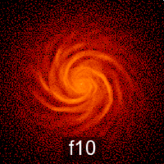
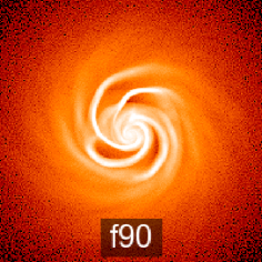
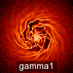
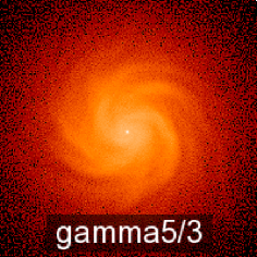
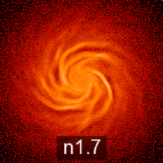
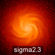
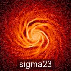
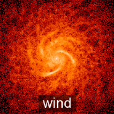
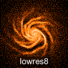
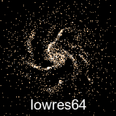
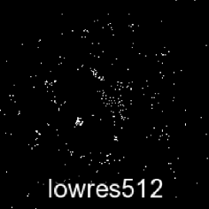
Table 1 lists all the simulations we have carried out and gives the values of all the parameters that are varied. Our fiducial simulation is labelled fid. Models f10 and f90 use initial disc gas fractions of 10 and 90 percent, respectively, compared with 30 percent for our fiducial model. The number of particles used in these runs is scaled accordingly, so that the particle mass remains constant. Models gamma1 and gamma5/3 use effective polytropic indices $\gamma_{\rm eff}=1$ and $5/3$ (i.e. isothermal and adiabatic), respectively, rather than our default value of $4/3$. Run n1.7 uses $n=1.7$ as the power-law index of the KS law instead of our default value of 1.4. Models sigma2.3 and sigma23 have threshold volume densities that are an order of magnitude lower and higher, respectively, than our default value of $n_{\rm H,c}=0.1~{}{\rm cm}^{-3}$. Because we keep $T/\mu$ at the threshold fixed, this yields critical surface densities that differ by $\sqrt{10}$ from the fiducial value (see eq. 7). Model wind includes galactic winds, whereas the fiducial model does not. Our recipe for generating galactic winds will be described elsewhere, but we note here that it results in much stronger perturbations to the galaxy than the widely used model of Springel & Hernquist (2003). Finally, runs lowres8, lowres64, and lowres512 use particle masses that are greater than those used in our fiducial model by factors of 8, 64 and 512, respectively. The spatial resolution (i.e. the gravitational softening length) is increased by factors of 2, 4 and 8, respectively.

Figure 2: Face-on projections of the disc gas surface densities for all models listed in Table 1. All images are $20~{}h^{-1}\,\mbox{kpc}$ on a side, use the same logarithmic colour scale, and correspond to time $t=10^{2}$ Myr. The stellar disc, bulge and the halo are not shown. Each panel is labelled by the model ID, as used in Table 1.

Figure 3: Comparison of the SF histories of the different simulations. The thick solid line in each plot shows the SF history of our fiducial model, fid. The other curves are labelled in the legends of the individual panels.

4.3 Results

4.3.1 Global properties

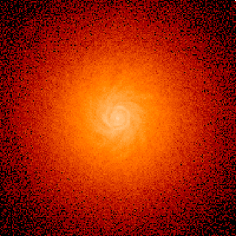
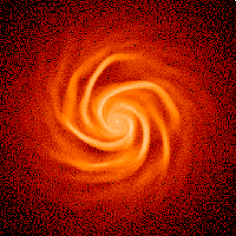
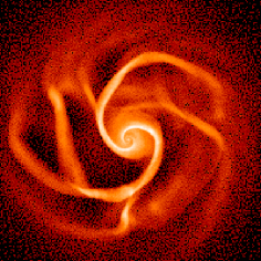
Figure 1 shows how our fiducial model evolves. From left to right, the panels show face-on projections of the disc gas distribution at times 25, 125, and 250 Myr after the start of the run. Spiral arms develop rapidly, even though the discs were initially axisymmetric. By time $T=250$ Myr, the spiral arms are starting to fragment.

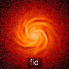
Figure 2 compares the face-on projections of the disc gas surface density for all runs. Because our galaxies have a fixed disc mass, a higher gas fraction implies higher gas surface densities, which results in sharper spiral arms. Increasing the polytropic index makes the galaxies more diffuse, which is not surprising given that both the Jeans length (22) and mass (23) are increasing functions of $\gamma_{\rm eff}$. On the other hand, model gamma1, which uses an isothermal effective equation of state, becomes unstable and fragments in small clumps. The same behaviour is visible in the models of Li et al. (2005) and Springel, Di Matteo, & Hernquist (2005). As we will demonstrate below, this simulation reproduces the desired local KS law, despite the strong instability. Increasing the slope of the KS law does not have much effect on the morphology of the galaxy. Including galactic winds makes the spiral arms more diffuse and results in the generation of low density bubbles in the outer disc. Increasing (decreasing) the SF threshold results in sharper (more diffuse) spiral arms. Again, this can be understood in terms of the Jeans scales, which decrease with the gas density. While model lowres8 still looks reasonably smooth, spurious fragmentation is visible in runs lowres64 and particularly in lowres512.

We show in Figure 3 a comparison of the SF histories integrated over the entire galaxy from $t=0$ till $t=400$ Myr, which is when we stopped the runs. The SFR of the fiducial simulation declines gently due to gas consumption. The same behaviour is seen in most of the other runs, with the exception of the models that we showed to be unstable in Fig. 2, gamma1 and lowres512, as well as f90 which becomes unstable shortly after the snapshot shown in Fig. 2. For these unstable models the SFR increases due to fragmentation, although gas consumption eventually forces it to decline.

Models f10 and f90 have initial gas fractions that differ by a factor of 3 from model fid. Since the total disc mass is fixed, this means that the gas surface densities differ by the same factor. Neglecting the change in the total gas mass above the SF threshold, which is justified since the SFR is dominated by dense gas, we would expect the SFRs to differ initially by about a factor $3^{1.4}$. This corresponds to 0.67 dex and agrees nearly perfectly with the simulation results.

The SF history of model sigma2.3, which has a critical surface density smaller than the fiducial model by 0.5 dex, is nearly indistinguishable from that of the fiducial run. This is because surface densities below the fiducial threshold contribute very little to the total SFR. As expected, model sigma23 is initially below the fiducial one because of the higher SF threshold. As the gas collapses to higher densities, so does the total gas mass above the threshold surface density. The SFR therefore increases slightly, temporarily surpassing that of model fid because it is forming stars in gas at higher surface densities, until gas consumption forces it to decline.

Run gamma5/3, which has a stiffer equation of state, is very similar to model fid. Note, however, that ab initio models (i.e. simulations which model the formation of galaxies) could still show significant differences between the SF histories of simulations using different equations of state. This would, however, not mean that the predicted KS laws are different, which we shall show below is not the case. It would merely indicate that the equation of state affects the gas distribution. Indeed, run gamma1, which has a softer equation of state, has a much higher SFR because the gas distribution changed as a result of fragmentation. But, as we shall show below, the local KS law still holds.

Decreasing the mass (spatial) resolution by a factor 8 (2) does not result in a significantly different SF history, indicating that our fiducial simulation has converged. Decreasing the resolution further does, however, lead to differences because the disc becomes unstable. Again, we shall see that this does not imply that the KS laws differ.

Increasing the slope of the KS law naturally leads to a higher SFR, although it eventually drops below the fiducial rate due to the fast gas consumption. Finally, including feedback from SF in the form of winds reduces the SFR. It takes some time for the difference to develop because the initial conditions were the same, i.e., the starting point is not affected by the winds.

4.3.2 Local properties

Figure 4: KS law for simulations f10 (left panel), fid (middle panel) and f90 (right panel) at $t=100~{}\mbox{Myr}$. Filled circles indicate SFR per unit area as a function of the gas surface density, both averaged azimuthally in radial bins containing a a fixed gas mass. The dot-dashed lines show the input KS law and threshold surface density for the fiducial simulation. The dotted lines show the expected scaling with the gas fraction (see the text for details). Data points with $\dot{\Sigma}_{\ast}<10^{-6}~{}\mbox{M}_{\sun}\,\mbox{yr}^{-1}\,\mbox{kpc}^{-2}$ are set equal to this value for clarity. The agreement between the input SF law and the simulation results is clearly excellent.

Figure 5: As Fig. 4 but for simulations gamma5/3 (left panel), gamma1 (middle panel) and gamma1 with cylindrical binning (right panel). The local KS law reproduces the input law everywhere, but for unstable regions of the disc this is only visible if we use local bins rather than azimuthal averages.

We now come to the most relevant results from the simulations, the SF threshold and the local KS law. Unless noted otherwise, we tested the KS law by projecting the gas density and SFR along the minor axis, and measuring their values in radial, concentric bins containing a fixed gas mass (corresponding to 2000 particles for run fid). For comparison, we explored two other ways of binning the data: radial bins spanning an azimuthal angle $\Delta\phi\ll 2\pi$ and randomly distributed cylinders containing a fixed number of particles. All three methods give nearly identical results if the disc is stable. All plots in this section are for $t=100$ Myr and can therefore be compared directly to Figure 2.

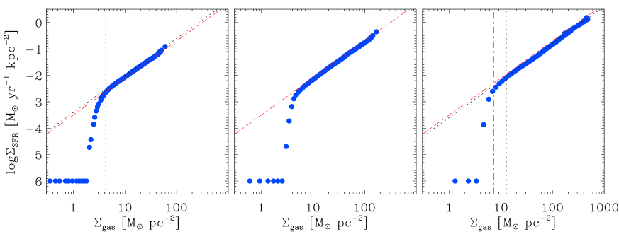
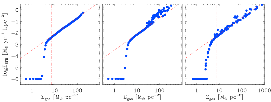
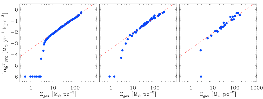
The data points in Figure 4 show the SFR per unit area as a function of the gas surface density, both averaged azimuthally, for simulations f10, fid and f90. In this figure and also in the remaining ones, all bins for which $\dot{\Sigma}_{\ast}<10^{-6}~{}\mbox{M}_{\sun}\,\mbox{yr}^{-1}\,\mbox{kpc}^{-2}$ have been set equal to this value for clarity. The red dot-dashed lines are not fits to the data points, but show the input KS law and SF threshold.

The agreement between the simulation results and the input KS law is nearly perfect, both in terms of its normalisation and slope. In fact, the agreement is better than could have been expected, given that the analytic formulas derived in §2.2 are no more accurate than the arbitrariness in the definition of the Jeans length, roughly a factor $\sqrt{\pi}$. However, from equations (7) and (14), we can see that this would only change the normalisation of the Schmidt law by a factor $\pi^{(n-1)/2}$, which is 0.1 dex for $n=1.4$, and that the slope would not be affected at all. Furthermore, S04 showed that for our definition of the Jeans length, (7) agrees with the exact solution for an isothermal, gaseous disc to within 2 percent.

The SFR clearly declines relatively sharply below a surface density threshold that is in good agreement with the input value. The fact that the agreement is less good for the threshold than for the KS law is not unexpected. For a fixed volume density, the corresponding surface density is proportional to the Jeans length. Therefore, discrepancies of the order of $\sqrt{\pi}$ (0.6 dex) are to be expected, but the difference is actually somewhat smaller than that, Note that the sharpness of the radial cut off in the SFR is sensitive to the way in which the simulation results are binned. Because the galaxies are not axisymmetric, azimuthal averaging smooths out the threshold, even if it is sharp locally.

All three simulations use the same values for the threshold volume density $\rho_{\rm g,c}$ and for the normalization of the SF law. That is, we always used the fiducial value $f_{\rm g}=0.3$ for the calculation of $\rho_{\rm g,c}$ from the input surface density threshold using equation (7), and also in the implemented KS law, equation (20). We neglected the weak dependence of the SF law on the gas fraction because we only know the initial disc gas fraction. The gas fraction appearing in the equations depends on both radius (due to the non-negligible contribution of the bulge near the center and the dark halo in the outer parts) and time (due to gas consumption).

The dotted lines in the left and right panels of Fig. 4 show the expected SF threshold and KS law assuming that the gas fraction appearing in the equations is identical to the initial disc gas fraction. As for the uncertainty due to the arbitrariness in the definition of the Jeans length, the dependence on the gas fraction is only significant for the critical surface density and even here it is weak. While run f10 reproduces the expected threshold better if the gas fraction is taken into account, the opposite is true for run f90. It appears that the initial disc gas fraction does change the threshold surface density, but the effect is weaker than the naive scaling indicated by the dotted lines.

Changing the effective equation of state of the star forming gas has the largest impact on the appearance of the gas disc (Fig. 2). Figure 5 shows the adiabatic (gamma5/3, left panel) and isothermal (gamma1, middle panel) runs, which can also be compared with the fiducial model shown in the middle panel of Fig. 4. The adiabatic and fiducial runs are nearly identical and both agree extremely well with the input SF law. This shows that we have succeeded in implementing local KS laws in a way that is independent of the effective equation of state. Clearly, in this respect our analytic theory describes the simulated galaxies very well.

At first sight, the isothermal run (middle panel) appears to overestimate the SFR by factors of a few for high surface densities ($\Sigma_{\rm g}>20~{}\mbox{M}_{\sun}\,\mbox{pc}^{-2}$). The disagreement is limited to the region of the disc that is unstable (Fig. 2). However, what we are seeing here is not a break-down of our theory, but rather an artifact caused by azimuthal smoothing. In the unstable region the departures from axisymmetry become very large and, at a fixed radius, the surface density fluctuates strongly. Because the KS law is supra-linear ($n>1$), azimuthal averaging will result in the inference of a steeper KS law.

We can remedy the binning problem by avoiding azimuthal smoothing. In the right panel of Fig. 5 we show the results for cylindrical binning. We use an equal number of bins as in the other panels, but center them on randomly chosen gas particles. For each bin we average $\dot{\Sigma}_{\ast}$ and $\Sigma_{\rm g}$ over a cylinder that contains a fixed number of particles. We chose bins of 100 particles as a compromise between the need to suppress noise (smaller for bigger bins) and the need for small spatial bins (using $\gg 100$ particles per bin leads to the same problem as we had for azimuthal binning). Clearly, purely local binning, which is more appropriate but more noisy than azimuthal binning, reveals that even this manifestly unstable disc follows the local KS law exactly as predicted.

Figure 6 demonstrates that the success of our model is not confined to one particular form of the KS law. If we change the slope of the input law from $n=1.4$ (open data points) to $n=1.7$ (filled data points), the simulation still reproduces the expected relation. As before, the very small deviations at high surface densities are caused by the decrease in the gas fraction due to gas consumption. For model n1.7 this happens at a smaller surface density because it has a higher SFR (for fixed $\Sigma_{\rm g}$).

Figure 6: As Fig. 4 but for models n1.7 (filled circles) and fid (open circles). The prescription for SF can match different input slopes of the KS law.

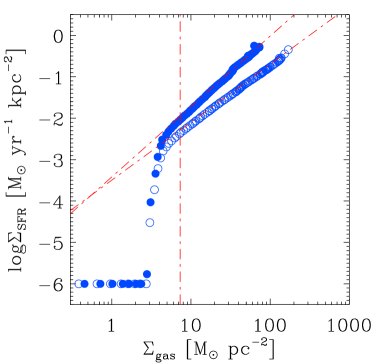
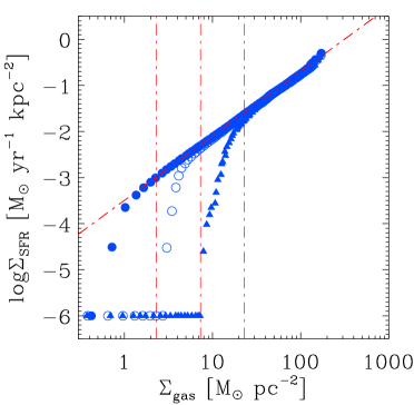
Figure 7 shows the effect of changing the surface density threshold. Comparing runs sigma2.3 (filled circles), fid (open circles) and sigma23 (filled triangles), it is clear that $\Sigma_{\rm c}$ scales as predicted.

Figure 7: As Fig. 4 but for models sigma2.3 (filled circles), fid (open circles) and sigma23 (filled triangles). The models match the desired SF thresholds.

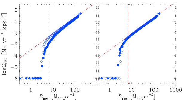
It may be argued that our model, which relies on the assumption that galaxy discs are self-gravitating, would break down for galaxies that are perturbed, although the results for the strongly unstable models suggest otherwise. It is therefore interesting to see how the model fares if we introduce a violent form of feedback from SF. As can be seen from Figures 2 and 3, our prescription for winds (which we will describe elsewhere) clearly has a dramatic effect on both the appearance and the SF history of the galaxy. Nevertheless, as is shown in the left panel of Figure 8, the simulation including winds (filled circles) still agrees with the input KS law with very little scatter. For surface densities around the threshold, the predicted SFR falls somewhat below the input KS law. The reason is that at these low densities the wind energy is dissipated sufficiently slowly that a significant part of the gas surface density is made up of ejected gas, which resides far above the disc and has volume densities that are too low to partake in the SF. In the right-hand panel of Figure 8 we again show models fid and wind, but this time we integrate only out to a scale height of 1 kpc. While this makes no difference for our fiducial model, it brings model wind in nearly perfect agreement with the input KS law.

Figure 8: As Fig. 4 but for models wind (filled circles) and fid (open circles). In the right hand panel $\dot{\Sigma}_{\ast}$ and $\Sigma_{\rm g}$ include only gas within a scale height of 1 kpc, while in the left panel we integrate to infinity, as was in the other figures. The model including galactic winds matches the input KS law very well, although it falls slightly below the fiducial model for densities around the threshold value. Excluding ejected gas (right panel) removes even this small discrepancy.

Finally, we show the results of a convergence test in Figure 9. Reducing the mass resolution by factors of 8 (lowres8, left panel), 64 (lowres64, middle panel) or even 512 (lowres512, right panel) does not undermine the agreement between the simulation results and the input SF law. This is quite remarkable, given that the two lowest resolution runs suffer strongly from spurious fragmentation (see Fig. 2). Note that the slight discrepancy for the lowest resolution model is most likely due to azimuthal binning (we cannot verify this because there are not enough particles for spatially resolved binning).

Figure 9: As Fig. 4 but for models lowres8 (left panel), lowres64 (middle panel) and lowres512 (right panel). The simulations match the input SF law, even for very low resolutions.

5 Discussion and conclusions

Star formation (SF) is poorly understood, but observations have revealed the existence of useful laws to describe its behaviour when averaged over scales that are large compared to individual star clusters. SF is suppressed if the local gas surface density falls below $\Sigma_{\rm c}\sim 3$–$10~{}\mbox{M}_{\sun}\,\mbox{pc}^{-2}$, while for higher densities a Kennicutt-Schmidt (KS) law, i.e. $\dot{\Sigma}_{\ast}\propto\Sigma_{\rm g}^{n}$, is a good description of the data. When averaged over entire galaxies, $n=1.4$ is a good fit and the same law may also hold locally, although this is less well established. If the local KS law is supra-linear ($n>1$), then the global law can only be identical if the total SF rate is dominated by a small region, e.g. the nucleus.

In S04 we provided a theoretical explanation for the existence of SF thresholds, showing that the surface density threshold for the formation of a cold gas phase agrees with the observationally determined SF threshold and that this transition triggers gravitational instability. S04 also provided a method for the implementation of arbitrary surface density thresholds in numerical simulations. Here, we have extended the work of S04 to KS laws. Although we have not offered an explanation for the observed KS law, we have provided a theory that relates various SF laws, that sheds new light on previous attempts to account for the observed KS law, and that enables the implementation of arbitrary SF laws into simulations of the formation and evolution of galaxies.

We showed that the KS law is primarily a pressure law since, as is well known, $\Sigma_{\rm g}\propto P_{\rm tot}^{1/2}$ for a self-gravitating disc, although the relation depends also on the gas fraction. The KS law is related to the Schmidt law, i.e. $\dot{\rho}_{\ast}\propto\rho_{\rm g}^{n_{S}}$, but the relation depends on the scale height and its dependence on the surface density. In general, the relation between surface and volume densities depends on the effective equation of state of the multiphase ISM and also on both the gas fraction and the fraction of the pressure that is thermal: $\Sigma_{\rm g}\propto f_{\rm g}^{1/2}f_{\rm th}^{-1/2}T^{1/2}\rho_{\rm g}^{1/2}$. For a polytropic effective equation of state, i.e. $P_{\rm tot}\propto\rho_{\rm g}^{\gamma_{\rm eff}}$, the power-law indices of the Schmidt and KS laws are related via $n=1+2(n_{S}-1)/\gamma_{\rm eff}$ if the gas fraction is independent of the density. More generally, the various SF laws, including their normalisations, can be related via the equations given in section 2.

Unless the SF laws are linear (i.e. $n=1=n_{S}$), the slopes of the Schmidt and KS laws will generally differ and the relation between the two will depend on the effective equation of state. Theoretical models have often ignored this difference and the dependence on the effective equation of state. For example, simulations and semi-analytic models typically assume a $n_{S}=1.5$ Schmidt law motivated by the fact that it implies a gas consumption time-scale proportional to the dynamical time ($\rho_{\rm g}/\dot{\rho}_{\ast}\propto\rho_{\rm g}^{-1/2}$) if, and this is sometimes forgotten, the SF efficiency per dynamical time is independent of the density. It is often mentioned that $n_{S}=1.5$ is also consistent with the observed KS law, $n=1.4\pm 0.1$. However, for $n_{S}=1.5$ to give $n=1.4$ we require $\gamma_{\rm eff}=2.5$ which is extreme and much greater than assumed/predicted by any of the simulations.

As long as simulations of galaxies lack the physics and/or resolution to model the multiphase ISM, in particular molecular cooling, radiative transfer, and efficient feedback from stellar winds and supernovae, they will require prescriptions for SF that can be calibrated to match observed scaling laws. We argued that such simulations should use an effective equation of state above the SF threshold, where the ISM is predicted to be multiphase. A polytropic index of $\gamma_{\rm eff}=4/3$ is particularly attractive from a numerical point of view since it results in a constant Jeans mass (and, for the case of SPH simulations, a constant ratio of the SPH kernel to the Jeans length), while the Jeans length still decreases with density. This choice therefore minimises resolution effects without directly suppressing collapse.

Because the observed SF laws involve surface densities whereas simulations require volume densities or pressures, our work is ideally suited for the implementation of arbitrary KS laws into simulations of galaxies. In particular, equation (18) expresses the star formation rate per resolution element in terms of its total total pressure and can thus be used even if the polytropic index depends on the density or if no effective equation of state is imposed.

Our equations enable us to predict many of the predictions of such simulations regarding large-scale SF laws, even though our theoretical framework does not explain why real galaxies follow such laws. The fact that we can predict simulation predictions once we know the sub-grid SF implementation, implies that simulations of galaxies that do not try to actually simulate the multiphase ISM, can only provide limited insight into the origin of the observed SF laws.

We discussed how to implement arbitrary KS laws into simulations that do not attempt to simulate the multiphase ISM and did so ourselves for the smoothed particle hydrodynamics code gadget. We used this code to test our analytical relations using high-resolution simulations of an isolated disc galaxy. We found that the simulations follow the predicted relations nearly perfectly. The surface density threshold and both the normalisation and the slope of the KS law are reproduced with hardly any scatter and without any tunable parameters. Moreover, this success is not limited to the SF laws that happen to describe the real universe, we can reproduce arbitrary input laws, again without tuning any parameters.

The agreement between theory and numerical experiment remains excellent if we include violent feedback from SF or use extremely low resolution. The only significant deviations that we found, occurred in unstable galaxies in which the spiral arms have fragmented. However, even these manifestly unstable galaxies turned out to follow the theoretical relations closely. The apparent discrepancy between the input and output SF laws turned out to be an artifact of azimuthal smoothing, which becomes inappropriate once the galaxy becomes fragmented.

Finally, we would like to stress that to better constrain the models, it is extremely important to get better observational constraints on the local SF threshold and the local KS law for a representative sample of galaxies. Even azimuthal smoothing should be avoided if at all possible, as it greatly confuses the comparison between theory and observations.

References

- Auld et al. (2006) Auld R., de Blok W. J. G., Bell E., Davies J. I., 2006, MNRAS, 366, 1475
- Bate & Burkert (1997) Bate M. R., Burkert A., 1997, MNRAS, 288, 1060
- Blitz & Rosolowsky (2006) Blitz L., Rosolowsky E., 2006, ApJ, 650, 933
- Boissier et al. (2006) Boissier S., et al., 2006, astro, arXiv:astro-ph/0609071
- Booth, Theuns, & Okamoto (2007) Booth C. M., Theuns T., Okamoto T., 2007, MNRAS, 376, 1588
- Cen & Ostriker (1992) Cen R., Ostriker J. P., 1992, ApJ, 399, L113
- de Blok & Walter (2006) de Blok W. J. G., Walter F., 2006, AJ, 131, 363
- Elmegreen (2002) Elmegreen B. G., 2002, ApJ, 577, 206
- Elmegreen & Parravano (1994) Elmegreen B. G., Parravano A., 1994, ApJ, 435, L121
- Ferland (2000) Ferland, G. J. 2000, Revista Mexicana de Astronomia y Astrofisica Conference Series, 9, 153
- Gerritsen & Icke (1997) Gerritsen J. P. E., Icke V., 1997, A&A, 325, 972
- Gnedin (1996) Gnedin N. Y., 1996, ApJ, 456, 1
- Guiderdoni (1987) Guiderdoni B., 1987, A&A, 172, 27
- Haardt & Madau (2001) Haardt, F., & Madau, P. 2001, to be published in the proceedings of XXXVI Rencontres de Moriond, astro-ph/0106018
- Hernquist (1990) Hernquist L., 1990, ApJ, 356, 359
- Heyer et al. (2004) Heyer M. H., Corbelli E., Schneider S. E., Young J. S., 2004, ApJ, 602, 723
- Katz (1992) Katz N., 1992, ApJ, 391, 502
- Katz, Weinberg, & Hernquist (1996) Katz N., Weinberg D. H., Hernquist L., 1996, ApJS, 105, 19
- Kauffmann, White, & Guiderdoni (1993) Kauffmann G., White S. D. M., Guiderdoni B., 1993, MNRAS, 264, 201
- Kawata & Gibson (2003) Kawata D., Gibson B. K., 2003, MNRAS, 340, 908
- Kay et al. (2002) Kay S. T., Pearce F. R., Frenk C. S., Jenkins A., 2002, MNRAS, 330, 113
- Kennicutt (1989) Kennicutt R. C., Jr., 1989, ApJ, 344, 685
- Kennicutt (1998a) Kennicutt R. C., Jr., 1998a, ARA&A, 36, 189
- Kennicutt (1998b) Kennicutt R. C., Jr., 1998b, ApJ, 498, 541
- Kennicutt et al. (2007) Kennicutt R. C., Jr., et al., 2007, arXiv, 708, arXiv:0708.0922
- Komugi et al. (2005) Komugi S., Sofue Y., Nakanishi H., Onodera S., Egusa F., 2005, PASJ, 57, 733
- Kravtsov (2003) Kravtsov A. V., 2003, ApJ, 590, L1
- Krumholz & McKee (2005) Krumholz M. R., McKee C. F., 2005, ApJ, 630, 250
- Li et al. (2005) Li Y., Mac Low M.-M., Klessen R. S., 2005, ApJ, 626, 823
- Li, Mac Low, & Klessen (2006) Li Y., Mac Low M.-M., Klessen R. S., 2006, ApJ, 639, 879
- Marri & White (2003) Marri S., White S. D. M., 2003, MNRAS, 345, 561
- Martin & Kennicutt (2001) Martin C. L., Kennicutt R. C., Jr., 2001, ApJ, 555, 301
- Maybhate et al. (2007) Maybhate A., Masiero J., Hibbard J. E., Charlton J. C., Palma C., Knierman K. A., English J., 2007, arXiv, 707, arXiv:0707.3582
- Meurer et al. (1996) Meurer G. R., Carignan C., Beaulieu S. F., Freeman K. C., 1996, AJ, 111, 1551
- Mihos & Hernquist (1994) Mihos J. C., Hernquist L., 1994, ApJ, 437, 611
- Mo, Mao, & White (1998) Mo H. J., Mao S., White S. D. M., 1998, MNRAS, 295, 319
- Olling (1995) Olling R. P., 1995, AJ, 110, 591
- Navarro & White (1993) Navarro J. F., White S. D. M., 1993, MNRAS, 265, 271
- Navarro, Frenk, & White (1996) Navarro J. F., Frenk C. S., White S. D. M., 1996, ApJ, 462, 563
- Okamoto et al. (2003) Okamoto T., Jenkins A., Eke V. R., Quilis V., Frenk C. S., 2003, MNRAS, 345, 429
- Quirk (1972) Quirk W. J., 1972, ApJ, 176, L9
- Schaye (2001a) Schaye J., 2001a, ApJ, 559, 507
- Schaye (2001b) Schaye J., 2001b, ApJ, 562, L95
- Schaye (2004) Schaye J., 2004, ApJ, 609, 667 (S04)
- Schaye (2007) Schaye, J. 2007, in IAU Symp. 244, arXiv:0708.3366
- Schmidt (1959) Schmidt M., 1959, ApJ, 129, 243
- Schuster et al. (2007) Schuster K. F., Kramer C., Hitschfeld M., Garcia-Burillo S., Mookerjea B., 2007, A&A, 461, 143
- Silk (1997) Silk J., 1997, ApJ, 481, 703
- Skillman (1987) Skillman E. D., 1987, sfig.conf, 263
- Sommer-Larsen, Götz, & Portinari (2003) Sommer-Larsen J., Götz M., Portinari L., 2003, ApJ, 596, 47
- Springel (2000) Springel V., 2000, MNRAS, 312, 859
- Springel, Yoshida, & White (2001) Springel V., Yoshida N., White S. D. M., 2001, NewA, 6, 79
- Springel & Hernquist (2003) Springel V., Hernquist L., 2003, MNRAS, 339, 289
- Springel (2005) Springel V., 2005, MNRAS, 364, 1105
- Springel, Di Matteo, & Hernquist (2005) Springel V., Di Matteo T., Hernquist L., 2005, MNRAS, 361, 776
- Steinmetz & Mueller (1994) Steinmetz M., Mueller E., 1994, A&A, 281, L97
- Summers (1993) Summers F. J., 1993, PhD thesis, Univ. California
- Tan (2000) Tan J. C., 2000, ApJ, 536, 173
- Tasker & Bryan (2006) Tasker E. J., Bryan G. L., 2006, ApJ, 641, 878
- Thacker & Couchman (2000) Thacker R. J., Couchman H. M. P., 2000, ApJ, 545, 728
- Toomre (1964) Toomre A., 1964, ApJ, 139, 1217
- Tutukov (2006) Tutukov A. V., 2006, ARep, 50, 526
- Wong & Blitz (2002) Wong T., Blitz L., 2002, ApJ, 569, 157
- Yepes et al. (1997) Yepes G., Kates R., Khokhlov A., Klypin A., 1997, MNRAS, 284, 235
- Zhang, Fall, & Whitmore (2001) Zhang Q., Fall S. M., Whitmore B. C., 2001, ApJ, 561, 727