Networks of Polynomial Pieces with Application to the Analysis of Point Clouds and Images

Abstract

We consider Hölder smoothness classes of surfaces for which we construct piecewise polynomial approximation networks, which are graphs with polynomial pieces as nodes and edges between polynomial pieces that are in ‘good continuation’ of each other. Little known to the community, a similar construction was used by Kolmogorov and Tikhomirov in their proof of their celebrated entropy results for Hölder classes.

We show how to use such networks in the context of detecting geometric objects buried in noise to approximate the scan statistic, yielding an optimization problem akin to the Traveling Salesman. In the same context, we describe an alternative approach based on computing the longest path in the network after appropriate thresholding.

For the special case of curves, we also formalize the notion of ‘good continuation’ between beamlets in any dimension, obtaining more economical piecewise linear approximation networks for curves.

We include some numerical experiments illustrating the use of the beamlet network in characterizing the filamentarity content of 3D datasets, and show that even a rudimentary notion of good continuity may bring substantial improvement.

Keywords and Phrases: Detection of filaments; Multiscale analysis; Beamlets; Extracting information from graphs; Hölder smoothness classes; Piecewise polynomials.

Acknowledgments: The authors are grateful to the anonymous referees and editors for their careful reading of an earlier version of the manuscript and their constructive comments. The first author was partially supported by NSF grant DMS-0603890.

1 Introduction

1.1 From function approximation to set approximation

An important trend in Approximation Theory and Harmonic Analysis focuses on designing dictionaries (e.g. orthonormal bases) $\{\phi_{n}\}$ well-adapted to a given function class ${\cal F}$, in the sense that any $f\in{\cal F}$ is well-approximated by a linear combination of a few functions from the dictionary:

$$f\doteq\sum_{n\in N(f)}a_{n}\phi_{n}.$$ (1)

Examples of dictionaries include the Fourier basis, polynomials, splines MR1045442 , radial basis functions, wavelets MR1614527 and others such as wedgelets wedgelets , platelets 1199635 , bandelets MR2128287 , rigelets MR1857974 , curvelets MR2012649 , chirplets chirp-tech .

In the context of function estimation in additive white noise johnstone1998feg ; MR1635414 ; MR1256530 , approximations by sums of atoms as in (1) are particularly suitable. Consider instead a setting where a geometric object (i.e. a set) is buried in noise or clutter, a setting considered e.g. in 2D-beamlets ; MGD . This is for example relevant in target tracking, where the object of interest is the target’s trajectory often modeled as a curve. In this setting, set approximation plays the role of function approximation, and the aim of the present paper is to develop strategies to compute approximations of sets by unions of simple building blocks akin to how beamlets are used to approximate curves in 2D-beamlets .

Since a set may be equivalently represented by its indicator function, approximation of sets may appear to be a special case of approximation of functions. Though indeed closely related, function approximation does not directly translate into set approximation. In part, this comes from the fact that the image of a sum of functions is in general not the union of the functions’ images. However, when a parametrization of the set is available, approximating the parametrization in piecewise fashion (i.e. when the supports of the functions involved in the sum do not overlap) does result in a proper approximation of the set itself. This is for example the case when the set is the graph of a function, considered in kor-tsy ; wedgelets in the context of image processing.

The selection of building blocks in set approximation is also not necessarily parallel to that of atoms in function approximation. The main difference is in the fact that overlapping building blocks create redundancy, while atoms with overlapping supports may cancel each other in appropriate ways to fit the target function, e.g. in trigonometric, polynomial or wavelet expansions. Typically, the approximation (1) is constructed by first computing the coefficients $a_{n}$, often as the inner product of $f$ and $\phi_{n}$, and then keeping the largest ones in absolute value, which is in effect equivalent to thresholding MR1256530 . A similar strategy may be implemented for sets, where building blocks with the most overlap with the set (as a fraction of their size) are selected; this corresponds to the simplest beamlet-based algorithm presented in 2D-beamlets . However, the result is often redundant, as nearby building blocks tend to have a similar overlap with a given set. This is avoided in the beamlet-based coder for curves introduced in 1518933 , by choosing at most one beamlet per dyadic square in a a given recursive dyadic partitioning. The strategy we adopt here consists of looking for a union of building blocks that obey some sort of ‘good continuation’. In the approximation of curves, this corresponds to the most complex algorithm presented in 2D-beamlets which amounts to chaining beamlets together that share one endpoint and have similar orientations. This is formalized in MSDFS for curves that are graphs of Hölder functions and in MR2379113 for chirps (highly oscillating functions), chaining chirplets in good continuation. Good-continuation principles are also considered in 766676 ; MR2036391 inspired by the Gestalt theory of vision, with applications to the detection of (parametric) geometric object in images.

1.2 Networks of polynomial pieces

We define a network of polynomial pieces to be a graph with nodes indexing polynomial pieces and edges between polynomial pieces in good-continuation. (We use the word ‘network’ instead of ‘graph’ so as to avoid confusion with the notion of ‘graph of a function’.) We construct such networks to approximate surfaces of varying dimension and smoothness. Just as beamlets are line-segments spanning a wide range of location, orientations and scale, so do the polynomial pieces. The networks are akin to that of MSDFS in that the notion of good-continuation is explicit and the scales are not mixed together, thus better adapted to surfaces with homogeneous smoothness, e.g. graphs of Hölder functions. We do, however, suggest ways to go multiscale.

In the 1950’s, Kolmogorov and Tikhomirov used piecewise polynomial approximations together with a similar kind of good-continuation notion to bound the $\epsilon$-entropy of Hölder function classes kolmogorov . Our construction may be seen as a formalization of their approach, with emphasis on the approximation of sets instead of functions. Note that this ancestry was discovered after the fact; the present perspective was indeed independently suggested in ery-thesis with the intention of generalizing the system used in MSDFS .

1.3 The special case of beamlets

Beamlets were introduced in 2D-beamlets for the explicit purpose of approximating curves in 2D, with a 3D version latter developed in 3D-beamlets . A variety of algorithms are proposed in 2D-beamlets , where the more elaborate ones are based on the chaining of beamlets in good continuation. However, the notion of good-continuation remains implicit and only palpable through numerical experiments.

We formalize here this notion of good-continuation for beamlets. This was previously done in MSDFS for a beamlet-like system built to detect graphs of Hölder functions. In the resulting beamlet network, small beamlets have a large number of neighbors; this seems unavoidable if the network is to enable accurate approximation of curves. To address this issue, we develop an alternative network of line-segments, with emphasis on developing an economical system both in terms of number of nodes and connectivity.

1.4 Application to the analysis of point clouds and images

1.4.1 Detection of geometric objects

Consider a simple model for detection, where we observe a point cloud (i.e. a spatial point process) and the goal is to decide whether the points were generated uniformly at random or a fraction of them were sampled from a geometric object (i.e. a surface) belonging to a given class.

This is a standard setting where the scan statistic is used GlaNauWal ; GlaBal , which consists in computing the largest number of points belonging to one of the objects of interest. Though the scan statistic achieves the best known detection rates, both for parametric MGD and nonparametric CTD classes of objects, it is not computationally friendly as it involves an optimization over a large (function) class of objects, though there are exceptions CTD-DP . Instead, we propose to replace the optimization over the class of objects with an optimization over paths in an approximating network. The idea of replacing an optimization over a function space with an optimization over a carefully constructed graph is quite natural, and in fact appears in other situations, e.g. in the computation of minimal surfaces 1238310 ; 10.1109/ICCV.2005.252 ; kirsanov2004dgm ; Hu_optimalminimum-surface . In our particular case, the resulting optimization problem is akin to the Budget-Reward problem DasHesSon ; though still NP-hard, this problem admits polynomial time approximations. Moreover, we show that this approximation achieves the best known detection rates.

Note that the optimization above is computationally more tractable (e.g. using dynamic programming ideas) when the network is direct and acyclic, which is the case for example in multiframe target tracking; see e.g. IMA_MFD , where a beamlet network is used to track the time-space primitives.

We also consider an alternative approach based on computing the size of the longest path in the network after thresholding, which is suggested in 2D-beamlets . Dynamic programming ideas may also be implemented here, as done in MSDFS . We show that this method also achieves the best known detection rates.

We mention that the same approaches may be implemented in the setting of an image, where a geometric object is buried in white Gaussian noise.

1.4.2 Characterization of spatial distributions

In Astrophysics, the study of the galaxy distribution involves quantifying the content in filaments, sheets and blobs in 3D galaxy catalogs MarSaa ; sdss . Ultimately, scientists would like to know which of the many cosmological models is best (and well) supported by observations. Practically, the task is to meaningfully compare simulated galaxy distributions from various cosmological models with the observed galaxy distribution.

With the presence of highly anisotropic features such as filaments, traditional tools for analyzing spatial data become irrelevant, among them the classical two-point correlation function. Instead, a method based on beamlets is very attractive, as beamlets provide good approximations for filaments. And indeed, spie-beamlets presents evidence that beamlets are useful at separating various cosmological models, even though the algorithm implemented in spie-beamlets is of the simplest kind and in particular does not involve chaining (i.e. good-continuation). We perform a number of numerical experiments on simulated data that show that chaining may bring substantial improvement.

Note that such tools are in demand in other scientific fields, such as Medical Imaging, for example in the examination of vascular networks APPLIC_3D_NETWORK or cancer cells APPLIC_FILAMENT_IN_CELLS .

1.5 Contents

The contents are organized as follow. In Section 2, we introduce piecewise polynomial networks designed to approximate surfaces of any intrinsic dimension and (Hölder) smoothness. In Section 3, we consider the detection of geometric objects buried in noise and develop methods based on these networks. In Section 4, we formalize a notion of good-continuation for beamlets in arbitrary dimension and show that the resulting network has desirable approximation properties for curves. In Section 5, we perform some numerical experiments showing that the notion of good-continuation may bring practical improvement. Some of the proofs and technical arguments are gathered in the Appendix.

2 Networks of Polynomial Pieces

We build an explicit, algorithmically friendly approximating network for Hölder surfaces, i.e. graphs or images of Hölder functions. As a Hölder function is well-approximated locally by a polynomial, in fact its Taylor expansion, it is natural to construct piecewise polynomial approximations. The idea is to partition the unit hypercube into smaller hypercubes and in each smaller hypercube provide a choice of approximation by polynomials; since the functions we consider are uniformly smooth, approximations in nearby hypercubes should be close, which we formalize as a neighboring condition. We thus form a network with nodes indexing polynomial pieces and edges linking those in good-continuation, restricting the possible combinations to those useful in approximating functions of given smoothness, in such a way that functions and certain connected components in this network are in correspondence. Though we build a different network for each smoothness class, it is possible to discretize the range of parameters resulting in a dyadic organization of this family of networks by scale.

Little known to the community, a similar construction was used by Kolmogorov and Tikhomirov in their seminal work on $\epsilon$-entropy of Hölder function classes (and others) MR0124720 ; kolmogorov . Note that the present construction was independently suggested in ery-thesis , as a generalization of the beamlet-like system used in MSDFS .

We first introduce some notation. For $i\in\{1,\dots,k\}$, let ${\bf e}_{i}$ denote the $i$th canonical vector in $\mathbb{R}^{k}$. For a vector ${\bf x}=(x_{1},\dots,x_{k})\in\mathbb{R}^{k}$, its supnorm is defined as $\|{\bf x}\|=\max\{|x_{i}|:i=1,\dots,k\}$. For ${\bf s}=(s_{1},\dots,s_{k})\in\mathbb{N}^{k}$, let ${\bf s}!=s_{1}!\cdots s_{k}!$ and $|{\bf s}|=s_{1}+\cdots+s_{k}$. For a function $f$ and ${\bf s}=(s_{1},\dots,s_{k})\in\mathbb{N}^{k}$, $f^{({\bf s})}=\partial_{x_{1}}^{s_{1}}\cdots\partial_{x_{k}}^{s_{k}}f$.

We define the following constants:

$$c_{1}=\sum_{|{\bf s}|=\lfloor\alpha\rfloor}\frac{1}{{\bf s}!},\qquad c_{2}=\sum_{|{\bf s}|\leq\lfloor\alpha\rfloor}\frac{2^{-|{\bf s}|}}{{\bf s}!}.$$ (2)

Note that $c_{1}\leq\exp(k)$ and $c_{2}\leq\exp(k/2)$.

2.1 Hölder smoothness classes

For $\alpha,\beta>0$, define ${\cal H}^{k}(\alpha,\beta)$ as the Hölder smoothness class of $\lfloor\alpha\rfloor$-times differentiable functions functions $f:[0,1]^{k}\rightarrow[0,1]$ satisfying:

$$|f^{({\bf s})}({\bf x})| \leq\beta,\quad\forall{\bf x}\in[0,1]^{k},\ \forall{\bf s}\in\mathbb{N}^{k},|{\bf s}|\leq\lfloor\alpha\rfloor;$$ (3)

$$|f^{({\bf s})}({\bf y})-f^{({\bf s})}({\bf x})| \leq\beta\|{\bf y}-{\bf x}\|^{\alpha-\lfloor\alpha\rfloor},\quad\forall{\bf x},{\bf y}\in[0,1]^{k},\ \forall{\bf s}\in\mathbb{N}^{k},|{\bf s}|=\lfloor\alpha\rfloor.$$ (4)

Example.

($k=1$, $\alpha\in(1,2]$)

$$|f^{{}^{\prime}}(x)| \leq\beta,\quad\forall x\in[0,1];$$

$$|f^{{}^{\prime}}(y)-f^{{}^{\prime}}(x)| \leq\beta|y-x|^{\alpha-1},\quad\forall x,y\in[0,1].$$

Functions in ${\cal H}^{k}(\alpha,\beta)$ are uniformly well-approximated locally by polynomials, specifically their Taylor expansions. For $f\in{\cal H}^{k}(\alpha,\beta)$ and ${\bf x}\in[0,1]^{k}$, the Taylor expansion of $f$ at ${\bf x}$ of degree $\lfloor\alpha\rfloor$ is defined as follows:

$$\dot{f}_{\bf x}({\bf y})=\sum_{|{\bf s}|\leq\lfloor\alpha\rfloor}f^{({\bf s})}({\bf x})\ \prod_{i=1}^{d}\frac{(y_{i}-x_{i})^{s_{i}}}{s_{i}!}.$$

Example.

($k=1$, $\alpha\in(1,2]$)

$$\dot{f}_{x}(y)=f(x)+f^{{}^{\prime}}(x)(y-x).$$

Lemma 2.1.

For any $f\in{\cal H}^{k}(\alpha,\beta)$,

$$|f({\bf y})-\dot{f}_{\bf x}({\bf y})|\leq c_{1}\beta\|{\bf y}-{\bf x}\|^{\alpha},\quad\forall{\bf x},{\bf y}\in[0,1]^{k}.$$

Proof.

A Taylor approximation of degree $\lfloor\alpha\rfloor$ gives:

$$f({\bf y})=\dot{f}_{\bf x}({\bf y})+\sum_{|{\bf s}|=\lfloor\alpha\rfloor}(f^{({\bf s})}({\bf z})-f^{({\bf s})}({\bf x}))\ \prod_{i=1}^{d}\frac{(y_{i}-x_{i})^{s_{i}}}{s_{i}!},$$

for some ${\bf z}$ on the segment joining ${\bf x}$ and ${\bf y}$. Hence,

$$|f({\bf y})-\dot{f}_{\bf x}({\bf y})|\leq c_{1}\|{\bf y}-{\bf x}\|^{\lfloor\alpha\rfloor}\max_{|{\bf s}|=\lfloor\alpha\rfloor}|f^{({\bf s})}({\bf z})-f^{({\bf s})}({\bf x})|.$$

Now apply (4) and the fact that $\|{\bf z}-{\bf x}\|\leq\|{\bf y}-{\bf x}\|$ to get

$$|f^{({\bf s})}({\bf z})-f^{({\bf s})}({\bf x})|\leq\beta\|{\bf y}-{\bf x}\|^{\alpha-\lfloor\alpha\rfloor},\quad\forall{\bf s}\in\mathbb{N}^{k},|{\bf s}|=\lfloor\alpha\rfloor.$$

∎

2.2 Nets of piecewise polynomials

We now build a family of nets for ${\cal H}^{k}(\alpha,\beta)$ by dividing $[0,1]^{k}$ into hypercubes and then offering a choice of approximation by polynomials within each hypercube, which is most relevant in view of Lemma 2.1. Fix $\Delta\in(0,1)$ and $\delta>0$, and define $\delta_{s}=\Delta^{-s}\delta,s=0,\dots,\lfloor\alpha\rfloor$. In the construction that follows, the parameter $\Delta$ quantizes the variable space, while each parameter $\delta_{s}$ quantizes the range of values of derivatives of order $s$ of functions in ${\cal H}^{k}(\alpha,\beta)$. Note that the quantization is coarser for higher order derivatives, and specifically chosen so that the approximation result in Lemma 2.2 below holds.

Divide $[0,1]^{k}$ into hypercubes indexed by ${\bf m}\in\{1,\dots,\Delta^{-1}\}^{k}$ of the form:

$$I_{\bf m} = \prod_{i=1}^{k}[(m_{i}-1)\Delta,m_{i}\Delta].$$

Let ${\bf x}_{\bf m}=(x_{{\bf m},1},\dots,x_{{\bf m},k})$ denote the center of $I_{\bf m}$, i.e. $x_{{\bf m},i}=(m_{i}-1/2)\Delta$. On each hypercube $I_{\bf m}$, consider polynomials of the form

$$p_{{\bf m},{\bf h}}({\bf x})=\sum_{|{\bf s}|\leq\lfloor\alpha\rfloor}h^{({\bf s})}\delta_{|{\bf s}|}\ \prod_{i=1}^{d}\frac{(x_{i}-x_{{\bf m},i})^{s_{i}}}{s_{i}!},$$ (5)

where ${\bf h}=(h^{({\bf s})}:|{\bf s}|\leq\lfloor\alpha\rfloor)$, with $h^{({\bf s})}\in{\mathbb{Z}}$ and $|h^{({\bf s})}\delta_{|{\bf s}|}|\leq\beta$.

Example.

($k=1$, $\alpha\in(1,2]$) For ${\bf h}=(h^{(0)},h^{(1)})$,

$$p_{m,{\bf h}}(x)=h^{(0)}\delta+h^{(1)}\delta_{1}(x-x_{m}).$$

(a) Linear

(b) Higher order

Figure 1: Examples of polynomial pieces for different choices of $\Delta$ and $\delta$, together with their associated region as defined in (8).

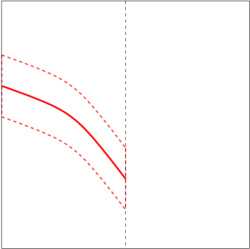
For $f\in{\cal H}^{k}(\alpha,\beta)$, let $h^{({\bf s})}({\bf m},f)$ denote the closest integer to $f^{({\bf s})}({\bf x}_{\bf m})/\delta_{|{\bf s}|}$.

Lemma 2.2.

For $f\in{\cal H}^{k}(\alpha,\beta)$ and ${\bf m}\in\{1,\dots,\Delta^{-1}\}^{k}$,

$$|f({\bf x})-p_{{\bf m},{\bf h}({\bf m},f)}({\bf x})|\leq(c_{1}/2^{\alpha})\beta\Delta^{\alpha}+(c_{2}/2)\delta,\quad\forall{\bf x}\in I_{\bf m}.$$

Proof.

The proof of Lemma 2.2 is in the Appendix. ∎

Partly justified by Lemma 2.2, we now assume that

$$\delta=c_{1}\beta\Delta^{\alpha}.$$ (6)

The system $\{p_{{\bf m},{\bf h}}\}$ is therefore rich enough to provide a certain degree of approximation locally. The same degree of approximation may be achieved globally by simply considering functions that coincide with the polynomials above within each hypercube, namely

$$g_{\bf h}({\bf x})=\sum_{{\bf m}}{\bf 1}_{\{{\bf x}\in I_{\bf m}\}}\ p_{{\bf m},{\bf h}({\bf m})}({\bf x}),$$

where this time ${\bf h}$ also depends on ${\bf m}$, representing a different choice for each hypercube.

As Kolmogorov and Tikhomirov realized, generating a $g_{\bf h}$ by simply picking a polynomial in each hypercube independently would result in a wasteful system, for in fact polynomials in neighboring hypercubes may be restricted to have similar coefficients. This comes from the fact that the derivatives up to order $\lfloor\alpha\rfloor$ of a function in $f\in{\cal H}^{k}(\alpha,\beta)$ have a certain degree of smoothness.

Lemma 2.3.

For $f\in{\cal H}^{k}(\alpha,\beta)$ and ${\bf s}$ such that $|{\bf s}|\leq\lfloor\alpha\rfloor$,

$$\left|f^{({\bf s})}({\bf x}+\eta{\bf e}_{i})-\sum_{t\leq\lfloor\alpha\rfloor-|{\bf s}|}f^{({\bf s}+t{\bf e}_{i})}({\bf x})\ \frac{\eta^{t}}{t!}\right|\leq c_{1}\beta\eta^{\alpha-|{\bf s}|},$$

for all ${\bf x}\in[0,1]^{k}$, $i=1,\dots,k$ and $\eta$ such that ${\bf x}+\eta{\bf e}_{i}\in[0,1]^{k}$.

Proof.

As with Lemma 2.1, perform a Taylor approximation of degree $\lfloor\alpha\rfloor-|{\bf s}|$ along ${\bf e}_{i}$ and apply (4). In fact, $\beta$ may be replaced by $\beta/(\lfloor\alpha\rfloor-|{\bf s}|)!$. ∎

2.3 Approximating networks for Hölder graphs

For a function $f:[0,1]^{k}\to[0,1]$, define its graph as

$${\rm graph}(f)=\{({\bf x},f({\bf x})):{\bf x}\in[0,1]^{k}\}.$$

Assuming (6), we define a network of polynomial pieces $\mathbb{G}_{\delta}^{k}(\alpha,\beta)$ with the property that a certain kind of connected components index piecewise polynomial approximations for graphs of Hölder functions. The network $\mathbb{G}_{\delta}^{k}(\alpha,\beta)$ has nodes of the form $({\bf m},{\bf h})$ indexing the polynomials $p_{{\bf m},{\bf h}}$ defined in (5). Two nodes in the network $({\bf m},{\bf h})$ and $({\bf m}_{\star},{\bf h}_{\star})$ are neighbors if the corresponding hypercubes, $I_{\bf m}$ and $I_{{\bf m}_{\star}}$, are adjacent, and if the corresponding polynomials, $p_{{\bf m},{\bf h}}$ and $p_{{\bf m}_{\star},{\bf h}_{\star}}$, and their derivatives assume nearby values both at ${\bf x}_{\bf m}$ and ${\bf x}_{{\bf m}_{\star}}$. Formally, this corresponds to ${\bf m}_{\star}={\bf m}+\xi{\bf e}_{i}$ for some $i\in\{1,\dots,k\}$ and $\xi\in\{-1,+1\}$, and for all ${\bf s}\in\mathbb{N}^{k},|{\bf s}|\leq\lfloor\alpha\rfloor$,

$$\left|h_{\star}^{({\bf s})}-\sum_{t\leq\lfloor\alpha\rfloor-|{\bf s}|}\frac{\xi^{t}}{t!}h^{({\bf s}+t{\bf e}_{i})}\right|<3\quad{\rm and}\quad\left|h^{({\bf s})}-\sum_{t\leq\lfloor\alpha\rfloor-|{\bf s}|}\frac{(-\xi)^{t}}{t!}h_{\star}^{({\bf s}+t{\bf e}_{i})}\right|<3.$$ (7)

This last property is a discrete version of Lemma 2.3.

Example.

($k=1$, $\alpha\in(1,2]$) The nodes $(m,h^{(0)},h^{(1)})$ and $(m_{\star},h_{\star}^{(0)},h_{\star}^{(1)})$ are neighbors if $|m_{\star}-m|=1$ and

$$|h_{\star}^{(1)}-h^{(1)}|<3,\quad|h_{\star}^{(0)}-h^{(0)}-(m_{\star}-m)h^{(1)}|<3,\quad|h^{(0)}-h_{\star}^{(0)}+(m_{\star}-m)h_{\star}^{(1)}|<3.$$

(a) In good continuation

(b) Not in good continuation

Figure 2: Examples of polynomial pieces in good continuation (left) and not in good continuation (right).

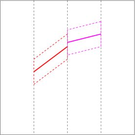
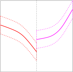
The family of networks $\mathbb{G}_{\delta}^{k}(\alpha,\beta)$ effectively generalizes the system presented in MSDFS for the case $k=1,\alpha\in(1,2]$.

Define constants

$$c_{3}=\sum_{s=0}^{\lfloor\alpha\rfloor}\left(\begin{array}[]{c}s+k-1\\ k-1\end{array}\right),\qquad c_{4}=\sum_{s=0}^{\lfloor\alpha\rfloor}s\left(\begin{array}[]{c}s+k-1\\ k-1\end{array}\right).$$

Lemma 2.4.

$\mathbb{G}_{\delta}^{k}(\alpha,\beta)$ has $O(\beta^{c_{3}}\delta^{-c_{3}}\Delta^{c_{4}-k})=O(\beta^{c_{3}-(c_{4}-k)/\alpha}\delta^{-c_{3}+(c_{4}-k)/\alpha})$ nodes and each node has at most $2k6^{c_{3}}$ neighbors.

Proof.

The proof of Lemma 2.4 is in the Appendix. ∎

Example.

($k=1$, $\alpha\in(1,2]$) $\mathbb{G}_{\delta}^{1}(\alpha,\beta)$ has $O(\beta\delta^{-2})$ nodes, each with degree at most 72.

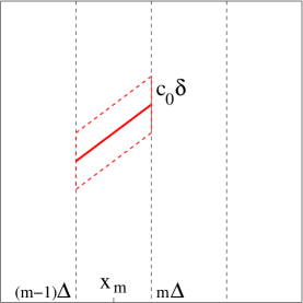
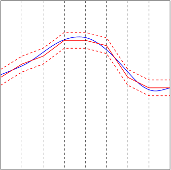
To each vertex $({\bf m},{\bf h})$ we associate a region around the graph of $p_{{\bf m},{\bf h}}$ restricted to $I_{\bf m}$, of thickness given by the error bound of Lemma 2.2:

$$R({\bf m},{\bf h})=\{({\bf x},z)\in I_{\bf m}\times[0,1]:|z-p_{{\bf m},{\bf h}}({\bf x})|\leq c_{0}\delta\},$$ (8)

where $c_{0}=(2^{-\alpha}+c_{2}/2)$. See Figure 1.

Example.

($k=1$, $\alpha\in(1,2]$) The regions are in this case parallelograms.

For a subset of nodes $\pi$, define $R(\pi)=\bigcup_{({\bf m},{\bf h})\in\pi}R({\bf m},{\bf h})$.

Let $\Pi_{\delta}^{k}(\alpha,\beta)$ denote the set of connected components of $\mathbb{G}_{\delta}^{k}(\alpha,\beta)$, homeomorphic to the square grid $\{1,\dots,\Delta^{-1}\}^{k}$.

Theorem 2.5.

For each $f\in{\cal H}^{k}(\alpha,\beta)$, there is a connected component $\pi\in\Pi_{\delta}^{k}(\alpha,\beta)$ such that ${\rm graph}(f)\subset R(\pi)$.

Proof.

The proof of Theorem 2.5 is in the Appendix. ∎

Figure 3: Example of covering of an Hölder graph (blue) with polynomial (linear) pieces in good continuation (red).

Theorem 2.5 implies that the system of functions

$$\sum_{({\bf m},{\bf h})\in\pi}{\bf 1}_{\{{\bf x}\in I_{\bf m}\}}\ p_{{\bf m},{\bf h}},\quad\pi\in\Pi_{\delta}^{k}(\alpha,\beta),$$

is an $\varepsilon$-net for ${\cal H}^{k}(\alpha,\beta)$ with $\varepsilon=c_{0}\delta$. From Lemma 2.4 and Theorem 2.5, we see that the system has entropy of order $O(\varepsilon^{-k/\alpha})$, which is essentially the smallest possible MR0124720 .

2.4 Approximating networks for Hölder immersions

Define ${\cal H}^{k,d}(\alpha,\beta)$ as the class of functions $f:[0,1]^{k}\rightarrow[0,1]^{d}$ with coordinates in ${\cal H}^{k}(\alpha,\beta)$, i.e. $f=(f_{1},\dots,f_{d})$ with $f_{r}\in{\cal H}^{k}(\alpha,\beta)$ for $r=1,\dots,d$.

For a function $f:[0,1]^{k}\to[0,1]^{d}$, define its image as

$${\rm im}(f)=\{f({\bf x}):{\bf x}\in[0,1]^{k}\}.$$

An approximation network for images of Hölder functions is simply built out of a tensor product of copies of the network built in the previous section. Specifically, define the network $\mathbb{G}_{\delta}^{k,d}(\alpha,\beta)$, with nodes of the form $({\bf m},{\bf h}_{1},\dots,{\bf h}_{d})$, indexing the multivariate polynomial $(p_{{\bf m},{\bf h}_{1}},\dots,p_{{\bf m},{\bf h}_{d}})$; and edges between nodes indexing polynomial pieces on adjacent hypercubes and satisfying (7) coordinate-wise.

Example.

($k=1$, $\alpha\in(1,2]$) The polynomial pieces are of the form:

$$(h_{1}^{(0)}\delta+h_{1}^{(1)}\delta_{1}(x-x_{m}),h_{2}^{(0)}\delta+h_{2}^{(1)}\delta_{1}(x-x_{m})),\quad|x-x_{m}|\leq\Delta/2.$$

Lemma 2.6.

$\mathbb{G}_{\delta}^{k,d}(\alpha,\beta)$ has $O(\beta^{dc_{3}}\delta^{-dc_{3}}\Delta^{dc_{4}-k})=O(\beta^{dc_{3}-(dc_{4}-k)/\alpha}\delta^{-dc_{3}+(dc_{4}-k)/\alpha})$ nodes and each node has at most $2k6^{dc_{3}}$ neighbors.

Proof.

The proof follows that of Lemma 2.4. Details are omitted. ∎

Example.

($k=1$, $\alpha\in(1,2]$) $\mathbb{G}_{\delta}^{1,2}(\alpha,\beta)$ has $O(\beta^{2-1/\alpha}\delta^{-4+1/\alpha})$ nodes, each with degree at most 2592.

As before, to each vertex $({\bf m},{\bf h}_{1},\dots,{\bf h}_{d})$ we associate a region around the image of $(p_{{\bf m},{\bf h}_{1}},\dots,p_{{\bf m},{\bf h}_{d}})$ restricted to $I_{\bf m}$, of thickness given by the error bound of Lemma 2.2:

$$R({\bf m},{\bf h}_{1},\dots,{\bf h}_{d})=\{{\bf z}\in[0,1]^{d}:\exists{\bf x}\in[0,1]^{k},\forall r=1,\dots,d,\ |z_{r}-p_{{\bf m},{\bf h}_{r}}({\bf x})|\leq c_{0}\delta\}.$$

Let $\Pi_{\delta}^{k,d}(\alpha,\beta)$ denote the set of connected components of $\mathbb{G}_{\delta}^{k,d}(\alpha,\beta)$, homeomorphic to the square grid $\{1,\dots,\Delta^{-1}\}^{k}$.

Theorem 2.7.

For each $f\in{\cal H}^{k,d}(\alpha,\beta)$, there is a connected component $\pi\in\Pi_{\delta}^{k,d}(\alpha,\beta)$ such that ${\rm im}(f)\subset R(\pi)$.

Proof.

The proof follows that of Theorem 2.5. Details are omitted. ∎

2.5 Networks organized by scale

In practice, the parameters $\alpha$ and $\beta$ are often unknown, so that it becomes necessary and/or useful to look through a discrete set. We introduce a scale parameter and another parameter indexing the approximation order, and organize the graphs accordingly. Fix $J\in\mathbb{N}$ as the maximum scale and a sequence $a_{J}\to\infty$ as $J\to\infty$. At scale $j\in\{0,\dots,J\}$ and approximation order $\iota\in\mathbb{N}$, let $\mathbb{G}_{j,J}^{k}(\iota)$ (resp. $\mathbb{G}_{j,J}^{k,d}(\iota)$) be defined as $\mathbb{G}_{\delta}^{k}(\alpha,\beta)$ (resp. $\mathbb{G}_{\delta}^{k,d}(\alpha,\beta)$) with $\lfloor\alpha\rfloor=\iota$, $\Delta=2^{-j}$, $\delta=2^{j-J}$ and $|h^{({\bf s})}\delta_{|{\bf s}|}|\leq a_{J}^{|{\bf s}|+1}$.

We have the following corollary of Theorems 2.5 and 2.7.

Proposition 2.8.

For $\alpha,\beta>0$, let $j=j(\alpha,\beta)=\lceil\frac{J+\log_{2}(c_{1}\beta)}{1+\alpha}\rceil$. Assume $J$ is large enough that $j(\alpha,\beta)\leq J$ and $a_{J}\geq\beta$. Also, take $\iota=\lfloor\alpha\rfloor$. Then the covering result of Theorem 2.5 (resp. Theorem 2.7) applies with $\mathbb{G}_{j,J}^{k}(\iota)$ (resp. $\mathbb{G}_{j,J}^{k,d}(\iota)$).

Proof.

This is a simple corollary of Theorems 2.5 and 2.7. ∎

2.5.1 A single multiscale network

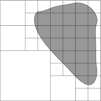
The networks $\mathbb{G}_{j,J}^{k}(\iota)$, $j=1,\dots,J$, $\iota\in\mathbb{N}$, constitute a family of monoscale networks. Instead, one may want to mix scales together (and possibly mix approximation orders too, though not done here) so as to better approximate functions with varying smoothness, akin to how Besov functions are decomposed into a sum of wavelets at various scales MR1228209 . Specifically, consider ${\cal F}^{k}(\iota)$ to be the class of $\iota$-times continuously differentiable functions of the form $f=\sum_{p\in P}f_{p}\chi_{p}$, where $P$ is a finite partition of $[0,1]^{k}$ into regions with boundaries of finite length and $f_{p}\in{\cal H}^{k}(\alpha_{p},\beta_{p})$ with $\alpha_{p}\in(\iota,\iota+1]$ and $\beta_{p}>0$. For such a function class, we may want to involve a number of scales, each adapted to a different smoothness degree.

In particular, such a multiscale approximating network may be built out of the union of $\mathbb{G}_{j,J}^{k}(\iota)$, $j=1,\dots,J$, with additional edges between nodes at different scales. The neighboring condition across scales may be chosen to be identical to that defined in Section 2.3, namely that $({\bf m},{\bf h})\in\mathbb{G}_{j,J}^{k}$ and $({\bf m}_{\star},{\bf h}_{\star})\in\mathbb{G}_{j_{\star},J}^{k}$ are neighbors if $I_{{\bf m}}$ and $I_{{\bf m}_{\star}}$ are adjacent, and if $p_{{\bf m},{\bf h}}$ and $p_{{\bf m}_{\star},{\bf h}_{\star}}$ together with their derivatives assume nearby values both at ${\bf x}_{\bf m}$ and ${\bf x}_{{\bf m}_{\star}}$. (The condition translates into a precise statement involving ${\bf h}$ and ${\bf h}_{\star}$ akin to (7), yet more cumbersome. We omit details.) Let $\mathbb{G}_{J}^{k}(\iota)$ denote this multiscale network.

Given a function $f\in{\cal F}^{k}(\iota)$, $f=\sum_{p\in P}f_{p}\chi_{p}$, we use a recursive dyadic partitioning (RDP), the cornerstone of many multiscale algorithms MR1614527 ; 2D-beamlets ; wedgelets ; MR2128287 , to approximate the partition $P$. Specifically, we start at $j=0$ and then recursively subdivide each dyadic hypercube $S$ at scale $j$ until $j\geq j(\alpha_{p},\beta_{p})$ for all $p\in P$ with $|p\cap S|>0$. We then use a polynomial piece from $\mathbb{G}_{j,J}^{k}(\iota)$ within each RDP cell at scale $j$. See Figure 4.

For a subset of nodes $\pi$ in $\mathbb{G}_{J}^{k}(\iota)$, define $R(\pi)=\bigcup_{({\bf m},{\bf h})\in\pi}R({\bf m},{\bf h})$, where each region is defined with the appropriate scale.

Proposition 2.9.

For each function $f\in{\cal F}^{k}(\iota)$, there is a connected component $\pi$ within $\mathbb{G}_{J}^{k}(\iota)$ in correspondence with an RDP such that ${\rm graph}(f)\subset R(\pi)$.

Proof.

This is essentially a corollary of Proposition 2.8. Details are omitted. ∎

Note however that the typical degree of a node in $\mathbb{G}_{J}^{k}(\iota)$ increases with $J$, as a result of connecting nodes across scales.

Figure 4: A partition into two regions $p_{1}$ (white) and $p_{2}$ (grey) associated with some function $f=f_{p_{1}}\chi_{p_{1}}+f_{p_{2}}\chi_{p_{2}}$, with corresponding scales $j(\alpha_{p_{1}},\beta_{p_{1}})=1$ and $j(\alpha_{p_{2}},\beta_{p_{2}})=3$.

3 Detection of Objects in Point Clouds and Images

We consider a simple model of detection of objects in point clouds and design some algorithms based on the networks introduced in Section 2. The objects are assumed to be of Hölder type. Fix an Hölder class ${\cal H}^{k,d-k}(\alpha,\beta)$. For $f\in{\cal H}^{k,d-k}(\alpha,\beta)$ and $\eta\geq 0$, define

$${\rm graph}_{\eta}(f)=\{({\bf x},{\bf z})\in[0,1]^{d}:\|{\bf z}-f({\bf x})\|\leq\eta\},$$

which is a region centered around the graph of $f$ and of thickness $2\eta$.

Suppose we observe a point cloud $X_{1},\dots,X_{n}\in[0,1]^{d}$, and want to decide between the following two hypotheses (generative models):

$$\begin{array}[]{rll}H_{0}:&\quad X_{1},\dots,X_{n}\sim^{\rm iid}&{\rm Uniform}[0,1]^{d};\\ H_{1}:&\quad X_{1},\dots,X_{n}\sim^{\rm iid}&(1-\varepsilon_{n}){\rm Uniform}[0,1]^{d}+\varepsilon_{n}{\rm Uniform}({\rm graph}_{\eta}(f^{*})),\\ &&\text{for some (unknown)}\ f^{*}\in{\cal H}^{k,d-k}(\alpha,\beta).\end{array}$$

The same situation was considered in MSDFS ; ery-thesis ; CTD .

For a (measurable) set $S\subset[0,1]^{d}$, let $N(S)$ denote the number of data points belonging to $S$, which under the null has the binomial distribution with parameters $n$ and $|S|_{d}$, the $d$-dimensional Lebesgue measure of $S$:

$$N(S)=\#\{i:X_{i}\in S\}\sim^{H_{0}}{\rm Bin}(n,|S|_{d}).$$

3.1 Generalized Likelihood Ratio Test

If $f^{*}$ were known, the most powerful test would be the likelihood ratio (i.e. Neyman-Pearson) test, which rejects for large values of $N({\rm graph}_{\eta}(f^{*}))$. The scan statistic is the maximum over those statistics:

$$M_{\eta}^{k,d}(\alpha,\beta)=\max_{f\in{\cal H}^{k,d}(\alpha,\beta)}N({\rm graph}_{\eta}(f)).$$

The generalized likelihood ratio test (GLRT) rejects when $M_{\eta}^{k,d}(\alpha,\beta)$ is large.

Define

$$\rho(k,d,\alpha)=\frac{k}{k+\alpha(d-k)}.$$

Theorem 3.1.

There are constants $A,B>0$ not depending on $n$ such that

$${\bf P}\left\{A(n^{\rho}\vee\eta^{d-k}n)\leq M_{\eta}^{k,d}(\alpha,\beta)\leq B(n^{\rho}\vee\eta^{d-k}n)|H_{0}\right\}\to 1,\quad n\to\infty.$$

Proof.

The lower bound is obtained by interpolation of carefully selected points, while the upper bound is obtained using a precise-enough net for ${\cal H}^{k,d-k}(\alpha,\beta)$ of near-optimal entropy (such as introduced in Section 2). We refer the reader to Section 2.3 in ery-thesis for more details. ∎

Since $M_{\eta}^{k,d}(\alpha,\beta)\geq N({\rm graph}_{\eta}(f^{*}))$ and ${\rm graph}_{\eta}(f^{*})$ contains at least an $\varepsilon_{n}$ proportion of the point cloud (roughly), the GLRT asymptotically separates $H_{0}$ and $H_{1}$ if, for some fixed $B^{\prime}>B$, $\varepsilon_{n}\geq B^{\prime}(n^{\rho}\vee\eta^{d-k}n)$, meaning that both the probabilities of false alarm (type I error) and missed detection (type II error) tend to zero as $n$ increases.

The GLRT as defined above is challenging, if not impossible to compute exactly. We use instead an approximation based on the coverings constructed in Section 2, turning an optimization over a functional space into an optimization over paths in a network, for which a large number of algorithms have been developed. See also kirsanov2004dgm ; 1238310 , where variational problems related to computing minimal surfaces are turned into combinatorial optimizations over paths and other structures within networks.

Recall the notation used in Section 2, and assume again that $\Delta$ and $\delta$ are related according to (6). We use the network $\mathbb{G}_{\delta}^{k,d-k}(\alpha,\beta)$ to build appropriate coverings, this time with slightly enlarged regions:

$$R_{\delta}({\bf m},{\bf h}_{1},\dots,{\bf h}_{d-k})=\{({\bf x},{\bf z}):{\bf x}\in I_{\bf m},\forall r=1,\dots,d-k,\ |z_{r}-p_{{\bf m},{\bf h}_{r}}({\bf x})|\leq(c_{0}+1)\delta\},$$

where $c_{0}=(2^{-\alpha}+c_{2}/2)$ as in (8).

Fix a path $\{{\bf m}_{\rm zz}(t):t=1,\dots,\Delta^{-k}\}$ in the square grid $\{1,\dots,\Delta^{-1}\}^{k}$ covering the whole grid in zig-zag fashion, and define ${\cal P}_{\delta}^{k,d-k}(\alpha,\beta)$ as the set of paths in $\mathbb{G}_{\delta}^{k,d-k}(\alpha,\beta)$ of the form

$$\{({\bf m}_{\rm zz}(t),{\bf h}_{1}(t),\dots,{\bf h}_{d-k}(t)):t=1,\dots,\Delta^{-k}\}.$$

Also, recall the definition of $\Pi_{\delta}^{k,d-k}(\alpha,\beta)$ in Section 2. Now consider the following alternative statistics:

$$M_{\Pi,\delta}^{k,d}(\alpha,\beta)=\max_{\pi\in\Pi_{\delta}^{k,d-k}(\alpha,\beta)}N(R_{\delta}(\pi)),\qquad M_{{\cal P},\delta}^{k,d}(\alpha,\beta)=\max_{P\in{\cal P}_{\delta}^{k,d-k}(\alpha,\beta)}N(R_{\delta}(P)).$$

In that case,

$$M_{\eta}^{k,d}(\alpha,\beta)\leq M_{\Pi,\delta}^{k,d}(\alpha,\beta)\leq M_{{\cal P},\delta}^{k,d}(\alpha,\beta).$$

The first inequality comes from Theorem 2.5 and the triangle inequality; the second from the fact that $\Pi_{\delta}^{k,d-k}(\alpha,\beta)\subset{\cal P}_{\delta}^{k,d-k}(\alpha,\beta)$. Actually, by Theorem 3.2 below, with a proper choice for $\delta$ all three are of same order of magnitude with high probability.

Theorem 3.2.

With $\delta=n^{-\alpha/(k+\alpha(d-k))}\vee\eta$, there is a constant $C=C(k,d,\alpha,\beta)$ such that

$${\bf P}\left\{M_{{\cal P},\delta}^{k,d}(\alpha,\beta)\leq C(n^{\rho}\vee\eta^{d-k}n)|H_{0}\right\}\to 1,\quad n\to\infty.$$

Proof.

The proof of Theorem 3.2 is in the Appendix. ∎

Computing $M_{{\cal P},\delta}^{k,d}(\alpha,\beta)$ may be done efficiently using dynamic programming ideas, for example as implemented in MR2379113 ; this is due to the fact that the paths in ${\cal P}_{\delta}^{k,d-k}(\alpha,\beta)$ are oriented and with no loops. Though $M_{\Pi,\delta}^{k,d}(\alpha,\beta)$ provides a better approximation to the scan statistic, we do not know of an efficient way to compute it directly.

The results above hold for Hölder immersions as well, though in that case the computations are much more challenging. This comes from the fact that Hölder immersions may self-intersect, so that dynamic programming approaches do not apply. In fact, if the optimization is over all paths of length $\Delta^{-k}$ instead, the setting is equivalent to the Budget-Reward Problem DasHesSon (also called Bank Robber Problem), closely related to the Prize-Collecting Traveling Salesman problem prize-collecting ; though those problems are known to be NP-hard, there are polynomial-time approximations DasHesSon . Other approaches have been suggested in this situation, for example in 2D-beamlets , where ratios of additive criteria are used to recover chains of beamlets; or algorithms implemented to extract curves from saliency networks 590008 ; 649458 .

3.2 Longest Significant Run

We propose an alternative approach based on the size of the longest path after discarding nodes with low counts within their associated region, which in effect generalizes the algorithm introduced in MSDFS .

For a threshold $\tau>0$, define

$$S({\bf m},{\bf h}_{1},\dots,{\bf h}_{d-k})=\left\{\begin{array}[]{ll}1,&N(R_{\delta}({\bf m},{\bf h}_{1},\dots,{\bf h}_{d-k}))>\tau n\delta^{k/\alpha+d-k},\\ 0,&\text{otherwise}.\end{array}\right.$$

Then define $L_{\tau}^{k,d}(\alpha,\beta)$ as the length of the longest path of the form

$$\{({\bf m}_{\rm zz}(t),{\bf h}_{1}(t),\dots,{\bf h}_{d-k}(t)):t=t_{0},\dots,t_{0}+\ell-1\},$$

such that $S({\bf m}_{\rm zz}(t),{\bf h}_{1}(t),\dots,{\bf h}_{d-k}(t))=1$ for all $t=t_{0},\dots,t_{0}+\ell-1$. If we see each $S({\bf m},{\bf h}_{1},\dots,{\bf h}_{d-k})$ as a test at node $({\bf m},{\bf h}_{1},\dots,{\bf h}_{d-k})$ and say that it is significant if it equals 1, then $L_{\tau}^{k,d}(\alpha,\beta)$ is the length of the longest significant run (LSR).

Theorem 3.3.

With $\delta=n^{-\alpha/(k+\alpha(d-k))}\vee\eta$, for $\tau$ large enough,

$${\bf P}\left\{L_{\tau}^{k,d}(\alpha,\beta)\leq\log(1/\delta)|H_{0}\right\}\to 1,\quad n\to\infty.$$

Also, there is a constant $C=C(k,d,\alpha,\beta)$ such that, if $\varepsilon>Cn^{\rho}\vee\eta^{d-k}n$,

$${\bf P}\left\{L_{\tau}^{k,d}(\alpha,\beta)>\log(1/\delta)|H_{1}\right\}\to 1,\quad n\to\infty.$$

Proof.

The proof of Theorem 3.3 is in the Appendix. ∎

Therefore, the LSRT achieves the detection rate established for the GLRT (Theorem 3.1) and its approximation (Theorem 3.2). Moreover, it can be computed using dynamic programming ideas since again the paths considered are oriented and without loops. This is done in MSDFS .

The same approach applies essentially unchanged to the case of Hölder immersions, though with pathological cases obscuring the exposition, so that we omit details.

A similar approach is advocated in water-quality , where a network of streams is monitored for pollution levels and large connected components of areas marked as problematic (polluted) are of interest. Two of the same researchers suggest a hybrid method in patil-upper applied to the identification of regions of interest (hot spots) in raster maps.

3.3 Detection in Grey-Level Images

The results we developed for point clouds can be obtained (in slightly different form) for digitized images, which is the context for the experiments of Section 5.

Suppose we observe a $d$-dimensional pixel array $Y$, with a total of $n$ pixels, of the form:

$$Y=\mu\ \xi_{{\rm graph}_{\eta}(f^{*})}+\sigma Z,$$

where $Z$ is white Gaussian noise, with independent, standard normal entries; $\sigma>0$ is the noise level; $\mu$ is the signal level; and for a subset $S\subset[0,1]^{d}$, $\xi_{S}$ is the array with $\ell^{2}$-norm 1 identifying the pixels that $S$ intersects, namely $\xi_{S}({\bf i})\propto{\bf 1}\{S\cap{\rm pixel}({\bf i})\neq\emptyset\}$.

We observe $Y$ and want to decide between $H_{0}$ and $H_{1}$ below:

$$\begin{array}[]{rll}H_{0}:&\quad\mu=0;\\ H_{1}:&\quad\mu>0,\text{ and }f^{*}\in{\cal H}^{k,d-k}(\alpha,\beta)\text{ is unknown}.\end{array}$$

This setting is considered in MGD (with a slightly different definition for $\xi_{S}$) in the context of parametric objects.

Following the same arguments as for point clouds, we find that the GLRT asymptotically separates $H_{0}$ and $H_{1}$ if $\mu\geq C(n^{k/(2\alpha d)}\vee\eta^{-k/(2\alpha)})$ with $C$ large enough, and that a detection threshold of same order of magnitude is achieved both by the approximate GLRT and the LSRT, with $\delta=\eta\vee n^{-1/d}$. We omit details.

4 Beamlet and Beamlet-Like Networks

We now focus on curves ($k=1$) of Hölder smoothness with $\alpha\in(1,2]$. The corresponding net described in Section 2 is made of piecewise linear functions. In this section, we show that such a net may be obtained by carefully chaining beamlets as suggested in 2D-beamlets , yielding a more economical net at a comparable degree of approximation.

The case of curves is special in the sense that it is the simplest, and in particular allows us to use a parametrization by arclength. Higher dimensional surfaces, even though smooth, may exhibit strange behavior, for example a very thin 2D surface in 3D.

4.1 Hölder Curves

We adopt here a slightly more intrinsic definition for curves. For $\alpha\in(1,2]$ and $\lambda,\kappa>0$, let $\Gamma(\alpha,\lambda,\kappa)$ be the set of curves $\gamma\subset[0,1]^{d}$ with ${\rm length}(\gamma)\leq\lambda$ and parametrized by arclength with

$$\|\gamma(t)-\gamma(s)-(t-s)\gamma^{\prime}(s)\|\leq\kappa\ |t-s|^{\alpha},\quad\forall s,t\in[0,{\rm length}(\gamma)].$$ (9)

$\Gamma(\alpha,\lambda,\kappa)$ is in close correspondence with ${\cal H}^{1,d}(\alpha,\beta)$ as defined in Section 2. Note that the case $\alpha=2$ includes all twice differentiable curves with curvature bounded by $2\kappa$.

Curves in $\Gamma(\alpha,\lambda,\kappa)$ satisfy the following properties.

Lemma 4.1.

For all $\gamma\in\Gamma(\alpha,\lambda,\kappa)$,

$$\|\gamma^{\prime}(t)-\gamma^{\prime}(s)\|\leq 2\kappa|t-s|^{\alpha-1},\quad\forall s,t.$$

Proof.

Fix $0\leq s<t\leq{\rm length}(\gamma)$. The triangle inequality and (9) give

$$(t-s)\|\gamma^{\prime}(t)-\gamma^{\prime}(s)\| \leq \|\gamma(t)-\gamma(s)-\gamma^{\prime}(s)(t-s)\|+\|\gamma(s)-\gamma(t)-\gamma^{\prime}(t)(s-t)\|$$

$$\leq 2\kappa(t-s)^{\alpha}.$$

∎

Lemma 4.2.

Let $\gamma\in\Gamma(\alpha,\lambda,\kappa)$. For all arclengths $r<s<t$,

$$\left\|\gamma(s)-\gamma(r)-\frac{s-r}{t-r}\ (\gamma(t)-\gamma(r))\right\|\leq 2\kappa(t-r)^{\alpha}.$$

Proof.

Applying (9) twice yields

$$\|\gamma(s)-\gamma(r)-(s-r)\gamma^{\prime}(r)\|\leq\kappa(s-r)^{\alpha}\leq\kappa(t-r)^{\alpha}$$

and

$$\left\|\frac{s-r}{t-r}\ (\gamma(t)-\gamma(r))-(s-r)\gamma^{\prime}(r)\right\|\leq\kappa\ (s-r)(t-r)^{\alpha-1}\leq\kappa(t-r)^{\alpha}.$$

Then apply the triangle inequality and conclude. ∎

4.2 Beamlets

Beamlets were introduced in 2D by Donoho and Huo 2D-beamlets , and then in 3D by Donoho and Levi 3D-beamlets ; spie-beamlets . We define them here in any dimension $d\geq 2$. Fix a maximum scale $J\in\mathbb{N}$. Define $\delta_{0}=2^{-J}$ and at scale $j\in\{0,\dots,J\}$, define $\Delta=2^{-j}$. For a given coordinate $r=1,\dots,d$, hyperplanes of the form

$$\{(x_{1},\dots,x_{d}):x_{r}=h\Delta\},$$

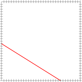
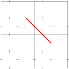
where $h\in\{0,\dots,\Delta^{-1}\}$, are called $r$-hyperplanes. Such hyperplanes will be called $\Delta$-hyperplanes; they partition the unit hypercube $[0,1]^{d}$ into smaller hypercubes of sidelength $\Delta$ that we call $\Delta$-hypercubes. On each $\Delta$-hyperplane, we consider a regular square grid with spacing $\delta_{0}$. Formally, we consider gridpoints of the form $(h_{1}\delta_{0},\dots,h_{d}\delta_{0})$, $h_{r}=0,1,\dots,\delta_{0}^{-1}$, with at least one coordinate an integer multiple of $\Delta\delta_{0}^{-1}$; if this happens at the $r$th coordinate, we speak of an $r$-gridpoint, which by definition belongs to an $r$-hyperplane. A beamlet is simply a line-segment joining two gridpoints belonging to the same $\Delta$-hypercube. See Figures 5.

(a) Coarsest scale, j=0

(b) Next finer scale, j=1

(c) Coarsest scale, j=0

(d) Next finer scale, j=1

Figure 5: Examples of beamlets in 2D and 3D.

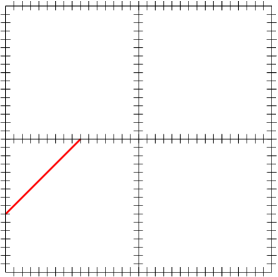
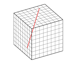
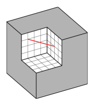
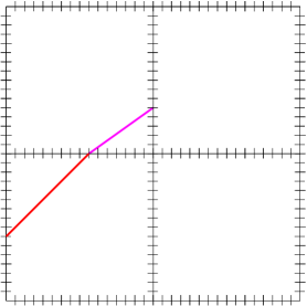
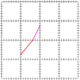
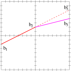
The beamlet graph in 2D-beamlets refers to the graph with nodes the gridpoints and edges the beamlets. Our interest instead is in building a beamlet good-continuation graph (i.e. network), with nodes the beamlets themselves and edges between beamlets in good-continuation, such that paths in that network provide a useful net for smooth curves. Such a graph is used in some experiments performed in 2D-beamlets , yet never formally defined there or elsewhere, though a related construction is presented in MSDFS for curves that are graphs of Hölder functions. Formally, two beamlets are neighbors if they are of the form $[b_{1},b_{2}]$ and $[b_{2},b_{3}]$ and satisfy

$$\|(b_{r,2}-b_{r,1})(b_{3}-b_{2})-(b_{r,3}-b_{r,2})(b_{2}-b_{1})\|$$

$$\qquad\qquad\qquad\qquad\qquad\qquad\leq 2^{j-J}(\|b_{3}-b_{2}\|+\|b_{2}-b_{1}\|),\quad\forall r=1,\dots,d.$$ (10)

This is basically a constraint on the angle formed by $[b_{1},b_{2}]$ and $[b_{2},b_{3}]$; see Figure 6.

Figure 6: Examples of 2D beamlets in good-continuation.

Let $\mathbb{B}_{j,J}^{d}$ denote the resulting beamlet good-continuation network at scale $j$.

Lemma 4.3.

The number of beamlets at scale $j$ is of order $\mathbb{B}_{j,J}^{d}=O(d^{2}2^{2(d-1)J-(d-2)j})$ and a given beamlet $B\in\mathbb{B}_{j,J}^{d}$ of length $|B|$ has $O(d|B|^{-(d-1)})$ neighbors.

Proof.

The proof of Lemma 4.3 is in the Appendix. ∎

Remark.

Short beamlets in the network $\mathbb{B}_{j,J}^{d}$ are highly connected. This is an undesirable feature and we were not able to avoid it, other than defining a closely related system in Section 4.3.

To each beamlet $B$ we associate a tubular region:

$$R(B)=\{{\bf x}\in[0,1]^{d}:\min_{{\bf y}\in B}\|{\bf x}-{\bf y}\|\leq 2^{j-J}\}.$$

We extend this definition to subsets of beamlets $R(\pi)=\bigcup_{B\in\pi}R(B)$.

Theorem 4.4.

Fix $\alpha\in(1,2]$ and $\lambda,\kappa>0$. Let $j(\alpha,\kappa)=\left\lceil\frac{\log_{2}(\kappa)+J}{\alpha+1}\right\rceil.$ There is a universal constant $K$ such that, when $J$ is large enough and $j\geq j(\alpha,\beta)+K$, to each curve $\gamma\in\Gamma(\alpha,\lambda,\kappa)$ corresponds a path $\pi_{j}$ in $\mathbb{B}_{j,J}^{d}$ chaining at most $(2d)(\lambda 2^{j}+2)$ beamlets such that $\gamma$ is included in $R(\pi_{j})$.

Proof.

Theorem 4.4 is a consequence of Theorem 4.6; see the comments following Theorem 4.6. ∎

Such a covering is illustrated in Figure 7.

Figure 7: Example of a curve (blue) approximation by a chain of 2D beamlets (red) in good continuation.

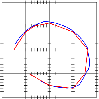
4.2.1 Multiscale beamlet good-continuation network

The chaining algorithms proposed in 2D-beamlets involve linking beamlets at different scales. Such a multiscale network may simply be constructed by taking the union of all $\mathbb{B}_{j,J}^{d},j=0,\dots,J$ and adding edges between beamlets at different scale satisfying (10) with $j$ replaced by the maximum of the two scales involved; see Figure 8. As in Section 2.5.1, an approximation is built using an RDP, this time of the ambient space $[0,1]^{d}$. Such a network provides more precise approximations to curves with varying smoothness, however at the cost of (substantially) increasing connectivity.

Figure 8: Example of 2D beamlets at different scales in good continuation.

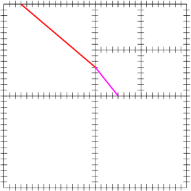
4.3 Beams

We found in Lemma 4.3 that defining a notion of good continuation directly between beamlets is problematic in that small corner beamlets become hubs, connected to a large number of other beamlets. The construction presented here uses other line-segments akin to beamlets, that we call beams. (Note that the term ‘beam’ refers to something else in 2D-beamlets .) Beams at a given scale are of similar length, thus avoiding the problem just mentioned, and each beam can be well approximated by a short chain of beamlets at that same scale.

Another drawback of beamlets as defined in Section 4.2 is that the quantization by $\delta_{0}$ does not change with the scale as $\Delta$ does; this results in a system that is more rich than needed, therefore wasteful. Just as in Section 2.5, at scale $j$ we define $\delta=2^{j-J}$, and $\Delta=2^{-j}$ as before; we assume that $j\leq J/2$, so that $\Delta$ is an integer multiple of $\delta$.

We define two kinds of beams. For $r=1,\dots,d$, an $r$-beam is a line segment joining two $r$-gridpoints $b_{1}$ and $b_{2}$ belonging to the same $\Delta$-hypercube on opposite sides, and such that

$$\|b_{1}-b_{2}\|\leq\Delta+\delta.$$ (11)

Therefore, an $r$-beam makes an angle of about 45 degrees or less with the $r$th axis.

For $r_{1},r_{2}=1,\dots,d$, with $r_{1}\neq r_{2}$, an $r_{1}r_{2}$-beam is a line segment joining an $r_{1}$-gridpoint $b_{1}$ and a $r_{2}$-gridpoint $b_{2}$ such that

$$\Delta\leq|b_{r_{1},1}-b_{r_{1},2}|\vee|b_{r_{2},1}-b_{r_{2},2}| <2\Delta,$$ (12)

$$\left|\ |b_{r_{1},1}-b_{r_{1},2}|-|b_{r_{2},1}-b_{r_{2},2}|\ \right| \leq\delta,$$ (13)

$$(|b_{r_{1},1}-b_{r_{1},2}|\vee|b_{r_{2},1}-b_{r_{2},2}|)-|b_{r_{3},1}-b_{r_{3},2}| \geq-\delta,\quad\forall r_{3}=1,\dots,d.$$ (14)

Note that $b_{1}$ and $b_{2}$ do not belong to the same $\Delta$-hypercube and that (14) is void in dimension $d=2$. Hence, an $r_{1}r_{2}$-beam connects an $r_{1}$-hyperplane and a $r_{2}$-hyperplane, making angles of about 45 degrees at the intersection with those hyperplanes. The reason $r_{1}r_{2}$-beams are so restricted is that they are only used to connect $r_{1}$-beams and $r_{2}$-beams.

(a) $r2$-beam ($j=0$)

(b) $r1$-beam ($j=1$)

(c) $r1r2$-beam ($j=2$)

Figure 9: Example of 2D beams.

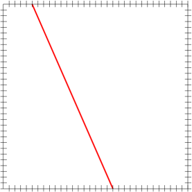
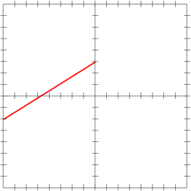
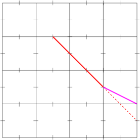
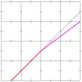
We define neighborhood relationships between beams as we did for beamlets in (10); see Figure 10. Specifically, two beams are neighbors if they are of the form $[b_{1},b_{2}]$ and $[b_{2},b_{3}]$ and satisfy

$$\|(b_{r,2}-b_{r,1})(b_{3}-b_{2})-(b_{r,3}-b_{r,2})(b_{2}-b_{1})\|$$

$$\qquad\qquad\qquad\qquad\qquad\qquad\leq(11\delta/20)(\|b_{3}-b_{2}\|+\|b_{2}-b_{1}\|),\quad\forall r=1,\dots,d.$$ (15)

For example, suppose $[b_{1},b_{2}]$ and $[b_{2},b_{3}]$ are both $r_{1}$-beams. If $b_{3}^{*}$ is the intersection of the line $(b_{1},b_{2})$ with the $r_{1}$-hyperplane $b_{3}$ belongs to, then condition (15) implies $\|b_{3}-b_{3}^{*}\|<(5/2)\delta$, so that $b_{3}$ is among the $5^{d-1}$ $r_{1}$-gridpoints closest to $b_{3}^{*}$.

(a) Two $h1$-beams

(b) $h1h2$-beam and $r_{1}$-beam

(c) Two $h1h2$-beams

Figure 10: Example of 2D beams in good continuation.

Let $\overline{\mathbb{B}}_{j,J}^{d}$ denote the resulting beam good-continuation network at scale $j$.

Lemma 4.5.

The number of nodes in $\overline{\mathbb{B}}_{j,J}^{d}$ is of order $O(d2^{2(d-1)J-(3d-4)j}(1+d2^{2j-J}))$. Moreover, all nodes have at most $2d\cdot 7^{d-1}$ neighbors, with most nodes having at most $2\cdot 5^{d-1}$ neighbors.

Proof.

The proof of Lemma 4.5 is in the Appendix.∎

Just as we did for beamlets, to each beam $B$ we associate a tubular region:

$$R(B)=\{{\bf x}\in[0,1]^{d}:\min_{{\bf y}\in B}\|{\bf x}-{\bf y}\|\leq\delta\}.$$

Theorem 4.6.

Fix $\alpha\in(1,2]$ and $\lambda,\kappa>0$. There is a universal constant $K$ such that, when $J$ is large enough and $j\geq j(\alpha,\beta)+K$, to each curve $\gamma\in\Gamma(\alpha,\lambda,\kappa)$ corresponds a path $\pi_{j}(\gamma)$ in $\overline{\mathbb{B}}_{j,J}^{d}$ chaining at most $\lambda 2^{j}+2$ beams such that $\gamma$ is included in $R(\pi_{j})$.

Proof.

The proof of Theorem 4.6 is in the Appendix. ∎

Figure 11: Example of a curve (blue) approximation by a chain of 2D beams (red) in good continuation.

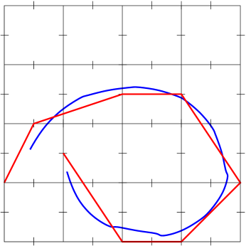
We now explain how Theorem 4.6 implies Theorem 4.4. First, any beam may be approximated within distance $\delta_{0}$ by a chain of at most $2d$ beamlets at the same scale. Indeed, a beam touches at most $2d$ $\Delta$-hyperplanes (at most $d+1$ for a typical $r$-beam); on each one, select a $(\Delta,\delta_{0})$-gridpoint closest to the beam. By successively connecting those gridpoints with line-segments, a chain of beamlets is born. Therefore, a chain of beams of length at most $\lambda 2^{j}+2$ may be approximated by a chain of beamlets of length at most $(2d)(\lambda 2^{j}+2)$. That the successive beamlets in such a chain are in good continuation according to (10) comes from the fact that the beams themselves are in good continuation according to (15), how beamlets are chained to approximate a beam, and the triangle inequality, in parallel to how Claim 3 is established in the proof of Theorem 4.6.

Remark.

Both $\overline{\mathbb{B}}_{j,J}^{d}$ and $\mathbb{G}_{j,J}^{1,d}$ provide $\varepsilon$-nets for Hölder curves embedded in the $d$-dimensional unit hypercube, with $\varepsilon$ of order $2^{j-J}$. Which one is more economical? In terms of number of nodes, $\log_{2}(|\mathbb{G}_{j,J}^{1,3}|)\sim 2dJ-(3d-1)j$ (Lemma 2.4), while $\log_{2}(|\overline{\mathbb{B}}_{j,J}^{d}|)\sim 2(d-1)J-(3d-4)j$ (Lemma 4.5); the latter is smaller for all relevant scales $j\leq J/2$. Perhaps more importantly, $\mathbb{G}_{j,J}^{1,d}$ is substantially more connected, with most nodes with $2\cdot 36^{d}$ neighbors (2592 in 2D; 93312 in 3D), compared to $\overline{\mathbb{B}}_{j,J}^{d}$, with most nodes having $2\cdot 5^{d}$ neighbors (50 in 2D; 250 in 3D).

5 Numerical Experiments

We perform some numerical experiments showing the power of approximation networks built on good-continuation principles. Specifically, we compare the filamentary content of simulated 3D datasets with a variety of beamlet-based algorithms of our own creation. Using software developed in shas and a basic notion of good-continuity as introduced in Section 4.2 is enough to outperform simpler algorithms disregarding any spatial information, such as introduced in spie-beamlets .

We consider three situations illustrated in Figure 12, where each column corresponds to a different case, and for each case the goal is to distinguish between the top and bottom situations. In setting (a), we compare a random point cloud (top) with a set of random filaments of different lengths, orientations and curvatures (bottom). In setting (b), we compare a set of random filaments (top) with a set of random filaments constrained to pass through a small number of hubs (bottom). In setting (c), we compare a set of short random filaments (top) with a set of long random filaments (bottom), all filaments oriented in the direction of the first coordinate.

Figure 12: Simulated datasets: (a) random point cloud (top) vs. random filaments (bottom); (b) random filaments (top) vs. random filaments with hubs (bottom); (c) random short filaments vs. random long filaments.

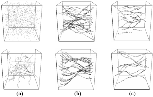
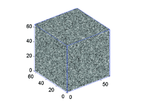
Each dataset is a pixel array of size $64^{3}$. The images are corrupted with a certain amount of additive white Gaussian noise (see Figure 13), calibrated so the algorithm introduced in spie-beamlets (and described in Section 5.4.1) is powerless, i.e. essentially useless at distinguishing between the top and bottom settings. All filaments in these datasets are synthesized using trigonometric functions, each with randomly selected location, amplitude, frequency and phase shift.

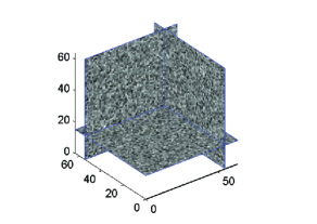(a) Surface of the noisy data volume	(b) Orthogonal slices through the noisy data

Figure 13: Noisy version of the simulated data in the lower panel of column (a) in Figure 12.

Though we introduce a variety of statistics, the workflow is the same:

1. Compute the beamlet transform. This amounts to computing all the beamlet coefficients, where a beamlet coefficient is defined as the line-integral of the image along the beamlet 2D-beamlets ; 3D-beamlets .

2. Thresholding of the beamlet coefficients. Beamlets with a large coefficient are suspected to be intersecting with a filament, and therefore informative since our objective involves detecting filaments. We therefore focus on those beamlets with large coefficients by discarding those with low coefficients 2D-beamlets ; 3D-beamlets . The choice of threshold is not determined in advance, rather a variety of thresholds are considered within some range.

3. Construction of a good-continuation network (GCN) for each scale. Based only on the beamlets surviving thresholding, neighboring relationships as introduced in Section 4.2 are considered.

4. Extraction of some relevant network statistics. We extract a number of statistics from the beamlet network that are sensitive to different degrees and kinds of filamentarity such as node and edge cardinality or connected components counts, centrality measures or even more sophisticated statistics based on path search in the network.

Our software is based on the beamlet transform as implemented in shas and graph algorithms from the LEDA library leda . Our code is available online code .

In what follows, we will say that a test or method is ‘powerful’ if it faithfully (more than 95% of the time) distinguishes between the top and bottom settings.

5.1 Number of Edges vs. Number of Nodes

Our simplest algorithm looks at how the number of edges and the number of nodes vary together as functions of the threshold used.

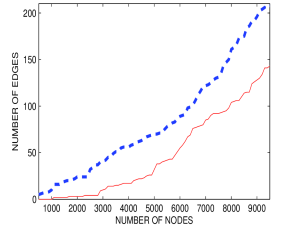
Consider column (a) of Figure 12, where we compare a random point cloud (top) with a set of filaments with random lengths, orientations and curvatures (bottom). In Figure 14, the number of edges is plotted as a function of the number of nodes for both top and bottom datasets. As expected, the curve corresponding to the random filaments rests above the curve corresponding to the random point cloud, since the GCN is more connected in the former setting. From our simulation studies, we found that this statistic is not powerful at per pixel signal-to-noise ratios (SNRs) below 0.8 for this specific situation. The dataset with filaments contains 20 of them with random lengths in the range $[10,64]$ (in number of pixels).

Figure 14: Number of edges vs. number of vertices for the random point cloud (red, solid curve) and the dataset of random filaments (blue, dashed curve) from column (a) of Figure 12.

5.2 Vertex Betweeness

Centrality attributes are well-known from network analysis networks_structure and used for example in social networks studies network_social . The betweeness of vertex $v$ is defined as

$$C_{B}(v)=\sum_{s\neq v\neq t}\frac{\rho_{st}(v)}{\rho_{st}},$$

where $s,t$ run through all vertices except $v$, $\rho_{st}$ is the number of longest paths from $s$ to $t$, and $\rho_{st}(v)$ the number of longest paths from $s$ to $t$ that pass through a vertex $v$. (Note that shortest paths are sometimes used instead.)

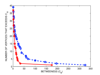
Consider column (b) in Figure 12, where the top image contains randomly distributed filaments and the bottom image also contains random filaments but with hubs. The number of filaments and their individual characteristics are the same in both cases. In Figure 15 we plot the number of vertices with betweeness exceeding a given threshold for both datasets. As expected, the curve corresponding to the random filaments with hubs rests above the curve corresponding to the random filaments without hubs, since in the former case the hubs translate into vertices in the GCN with large betweeness. From our simulation studies, we also found this statistic not powerful at SNRs below 0.8 for the type of filaments chosen here. The data set without hubs (top) contains 20 filaments with horizontal orientations and random lengths in range $[60,63]$. The data set with hubs contains 5 groups of 4 filaments with horizontal orientations and length 64, then all 4 filaments in the group have common filamentarity region of length 3 (hub).

Figure 15: Number of vertices whose betweeness exceeds a given threshold for the dataset of random filaments without hubs (red, solid) and the dataset of random filaments with hubs (blue, dashed) from column (b) of Figure 12.

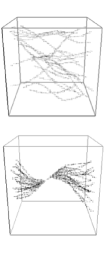
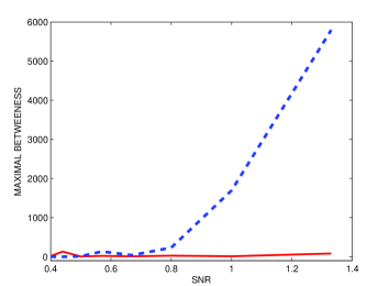
Now, consider a slightly different setting with just one large hub, illustrated in the left column of Figure 16. In the right column of the Figure 16 we compare the maximal betweeness of both datasets for different noise levels, which is significantly larger for the dataset with a hub. Again, we found that the maximal betweeness statistic is not effective when the voxel-level SNR is less than $0.8$. The data set without hub (top) contains 18 filaments with horizontal orientations and random lengths in range $[48,64]$. The data set with hub contains 18 filaments with horizontal orientations and length 64, then all filaments in the group have common filamentarity region of length 5 (hub).

Figure 16: Maximal betweeness as a function of SNR, for the dataset of random filaments without hub (red, solid) and the dataset of random filaments with a hub (blue, dashed) from the left column.

5.3 Filamentarity Survival Index

For each beamlet $v$ in the network, let $\omega(v)$ denote its coefficient (or weight), i.e. the line-integral of the image along this beamlet. The weight of a beamlet path $p$ is then defined as the sum of the weights of the beamlets it passes through:

$$\omega(p)=\sum_{v\in p}\omega(v).$$

Let $P$ be the partitioning of $\mathbb{G}$ into disjoint paths defined recursively as follows:

$$\left\{\begin{array}[]{l l}p_{1}=\arg\max_{p\in\mathbb{G}}\omega(p);\\ p_{i}=\arg\max_{p\in\mathbb{G}\backslash\{p_{1},\ldots,p_{i-1}\}}\omega(p),&\quad i>1.\end{array}\right.$$ (16)

We define the Filamentarity Survival Index $D(t)$ as the fraction of paths in $P$ with weight greater than $t$. The computation of the piecewise constant function $D(t)$ is iterative, where at each iteration the Longest Weighted Path (LWP) is found and removed from the network. The algorithm terminates when the network is empty.

We next define the Filamentarity Survival Ratio (FSR) which compares the filamentary survival index of a given dataset $I$ with the filamentary survival index a random point cloud with same energy, denoted $\tilde{I}$

$$R(t)=\frac{\left(D_{I}\left(t\right)+\epsilon\right)}{\left(D_{\tilde{I}}\left(t\right)+\epsilon\right)},$$

where $\epsilon$ is a small positive number, used to avoid divide-by-zero situations.

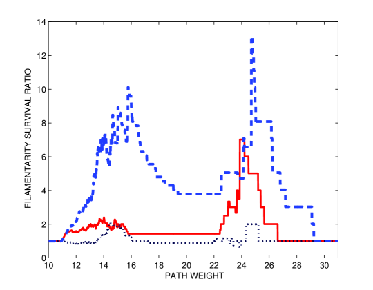
Consider column (c) in Figure 12, where we compare a dataset of random short filaments (top) with a dataset of random long filaments (bottom), all filaments oriented in the direction of the first coordinate. Figure 17 presents the FSR curves for these two datasets. Additionally, this figure contains the FSR curve for the case of purely random points, as in the top image in column (a) in Figure 12. As expected, the FSR curve for the purely random dataset (black, dotted line) remains close to 1. For the dataset containing long filaments, however, the FSR (blue, dashed line) is significantly higher than 1 for certain values of $t$. For the dataset containing short filaments, the FSR curve (red, solid line) is found between the other two curves. We found that the FSR statistic is powerless at distinguishing between short and long filaments (in this setting) for SNRs below 1 in this specific situation. The data set with short filaments (top) contains 30 filaments with horizontal orientations and lengths 20. The data set with long filaments (bottom) contains 10 filaments with horizontal orientations and lengths 60.

Figure 17: Filamentarity Survival Ratios for the dataset of random short filaments (red, solid) and for the dataset of random long filaments (blue, dashed) in column (c), and for the random point cloud (black, dotted) in column (a) of Figure 12.

5.4 Discussion

5.4.1 Comparison with statistics based on beamlet coefficients only

The numerical experiments we presented provide evidence that using the spatial relationship between beamlets allows for the design of algorithms that have the ability to perform well even in the case of very low SNR, where statistics based only on the beamlets coefficients fail. More precisely, we compared our different algorithms described above with the Log-Survival Index (LSI) introduced in spie-beamlets ; see Table 1. The LSI is defined as

$$S_{j}(t)=\frac{\log(1+N_{j}(t))}{\log(1+N_{j})},$$

where $N_{j}(t)$ is the number of beamlet coefficients at the $j$-th scale that exceed $t$, and $N_{j}$ is the total number of beamlet coefficients at scale $j$.

Case	(a)	(b)	(c)
Statistic	Graph connectivity	Vertex betweeness	FSR
Lowest SNR	0.8 (1.33)	0.8 (2)	1 (1.33)

Table 1: Summary of the experiments. The numbers (resp. numbers in parentheses) in the last row correspond to the lowest SNR at which the statistic used for that particular case (resp. the LSI statistic) is still powerful.

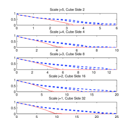
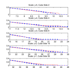
Figure 18 shows the behavior of this statistic for situation (a) of Figure 12. The LSI curves are clearly disjoint at SNR = 4; however, they merge at SNR = 0.8, resulting in the LSI being powerless, while the statistic presented in Section 5.1 is still powerful.

(a) SNR = 4

(b) SNR = 0.8

Figure 18: LSI curves at various scales for the random point cloud (red, solid) and for the dataset with random filaments (blue, dashed) in column (a) of Figure 12.

5.4.2 Computational Complexity

The computational burden comes from the beamlet transform. In these experiments, we used the version developed in shas , which runs in order $O(n^{5})$ flops for an $n^{3}$ pixel array. The version based on the Fast Slant Stack 3D-beamlets ; FSS is in theory faster, $O(n^{4}\log n)$ flops, yet in practice the implementation in shas is more precise and faster on smaller arrays as considered here.

We mention that beamlets have only been developed for 2D and 3D datasets, partly because the method suffers from the curse of dimensionality, since the number of beamlets increases exponentially with the ambient dimension; see Lemma 4.3. Note also that the implementation in 2D-beamlets runs in $O(n^{2}\log n)$ for an $n^{2}$ pixel array, so that the 3D implementations are comparatively heavier.

5.4.3 Computation of the Longest Weighted Paths

Since finding the LWP is an NP-Hard problem longest-path-NP , in the experiments described above we restricted ourselves to acyclic networks. We assume that the foreground signal consists of a set of curves of the form $\gamma(s)=(s,\gamma_{y}(s),\gamma_{z}(s))$. Therefore, it is possible to approximate such curves with beamlets oriented along the fist axis only, so their chaining will never induce a cycle. This rather artificial assumption was made only for computational reasons; for general datasets one would be forced to use approximations longest-path-approx or other strategies dp_tracking ; 2D-beamlets . We tried statistics based on connected components, which are computationally tractable, but were not able to improve on the LSI.

5.4.4 Full multiscale analysis

We built a good-continuation network for each scale separately along the lines presented in Section 4.2. Based on Theorem 4.6, this is fine if we expect filaments of homogenous smoothness. If we want to test for filaments of varying smoothness, building a single good-continuation network that includes neighboring relationships across scales may be more useful.

Appendix

Proof of Lemma 2.4

We first count the number of nodes $({\bf m},{\bf h})$. There are $\Delta^{-k}$ choices for ${\bf m}$ and $2\beta\delta_{|{\bf s}|}^{-1}$ for each $h^{({\bf s})}$, so for ${\bf h}$ a total of

$$\prod_{|{\bf s}|\leq\lfloor\alpha\rfloor}2\beta\delta_{|{\bf s}|}^{-1}=(2\beta)^{c_{3}}\delta^{-c_{3}}\Delta^{c_{4}}.$$

For a given node $({\bf m},{\bf h})$, ${\bf m}$ has at most $2k$ neighbors ${\bf m}_{\star}$’s in the square grid. And for each one of them, there are at most $6^{c_{3}}$ ${\bf h}_{\star}$’s satisfying the left part of (7), since at each ${\bf s}$ there are at most 6 choices.        $\Box$

Proof of Theorem 2.5

In view of Lemma 2.2, it is enough to show that, for ${\bf m},{\bf m}_{\star}\in\{1,\dots,\Delta^{-1}\}^{k}$ with ${\bf m}_{\star}={\bf m}+{\bf e}_{i}$,

$$\left|h^{({\bf s})}({\bf m}_{\star},f)-\sum_{t\leq\lfloor\alpha\rfloor-|{\bf s}|}\frac{h^{({\bf s}+t{\bf e}_{i})}({\bf m},f)}{t!}\right|<3.$$

By the triangle inequality, we have

$$\left|h^{({\bf s})}({\bf m}_{\star},f)-\sum_{t\leq\lfloor\alpha\rfloor-|{\bf s}|}\frac{h^{({\bf s}+t{\bf e}_{i})}({\bf m},f)}{t!}\right| \leq \left|h^{({\bf s})}({\bf m}_{\star},f)-\delta_{|{\bf s}|}^{-1}f^{({\bf s})}(x_{{\bf m}_{\star}})\right|+$$

$$\left|\delta_{|{\bf s}|}^{-1}f^{({\bf s})}(x_{{\bf m}_{\star}})-\sum_{t\leq\lfloor\alpha\rfloor-|{\bf s}|}\frac{\delta_{|{\bf s}|+t}^{-1}f^{({\bf s}+t{\bf e}_{i})}(x_{{\bf m}})}{t!}\right|+$$

$$\sum_{t\leq\lfloor\alpha\rfloor-|{\bf s}|}\frac{\left|\delta_{|{\bf s}|+t}^{-1}f^{({\bf s}+t{\bf e}_{i})}(x_{{\bf m}})-h^{({\bf s}+t{\bf e}_{i})}({\bf m},f)\right|}{t!}.$$

By definition of $h^{({\bf s})}({\bf m},f)$, the first term on the right handside is bounded by 1/2 while the third term is bounded by $1/2\ \sum_{t}1/t!\leq\exp(1)/2<3/2$. So we are left with showing that the second term is bounded by 1. To do that, we use Lemma 2.3 and the fact that $x_{{\bf m}_{\star},i}-x_{{\bf m},i}=\Delta$ to get

$$\left|f^{({\bf s})}(x_{{\bf m}_{\star}})-\sum_{t}f^{({\bf s}+t{\bf e}_{i})}(x_{{\bf m}})\ \frac{\Delta^{t}}{t!}\right|\leq c_{1}\beta\Delta^{\alpha-|{\bf s}|}.$$

Since $\Delta^{t}=\delta_{s}\delta_{s+t}^{-1}$ for all $s,t$, we further get

$$\left|\delta_{|{\bf s}|}^{-1}f^{({\bf s})}(x_{{\bf m}_{\star}})-\sum_{t}\frac{\delta_{|{\bf s}|+t}^{-1}f^{({\bf s}+t{\bf e}_{i})}(x_{{\bf m}})}{t!}\right|\leq c_{1}\beta\Delta^{\alpha}/\delta.$$

This concludes the proof of Theorem 2.5.        $\Box$

Proof of Theorem 3.2

We use simplified notation for clarity. By Boole’s Inequality, we have

$${\bf P}\left\{M_{\cal P}>C\delta^{d-k}n|H_{0}\right\}\leq|{\cal P}|\cdot\max_{P\in{\cal P}}{\bf P}\left\{N(R_{\delta}(P))>C\delta^{d-k}n|H_{0}\right\}.$$

For the number of paths,

$$|{\cal P}|=O(\delta^{-(d-k)c_{3}}\Delta^{(d-k)c_{4}}\cdot(6^{(d-k)c_{3}})^{\Delta^{-k}}),$$ (17)

since there are $O(\delta^{-(d-k)c_{3}}\Delta^{(d-k)c_{4}})$ choices for the starting point and $6^{(d-k)c_{3}}$ at each step after that, along a path of length $\Delta^{-k}$ (see Lemma 2.6). Hence, $\log(|{\cal P}|)\leq a_{1}\delta^{-k/\alpha}$ for some constant $a_{1}$ not depending on $\delta$.

Under $H_{0}$, $N(R_{\delta}(P))$ is binomial with parameters $n$ and $|R_{\delta}(P)|_{d}$, so that

$$\max_{P\in{\cal P}}{\bf P}\left\{N(R_{\delta}(P))>C\delta^{d-k}n|H_{0}\right\}={\bf P}\left\{{\rm Bin}(n,\max_{P\in{\cal P}}|R_{\delta}(P)|_{d})>C\delta^{d-k}n\right\}.$$

By integrating with respect to ${\bf z}$ (the last $d-k$ coordinates) first, we have:

$$|R_{\delta}({\bf m},{\bf h}_{1},\dots,{\bf h}_{d-k})|_{d}=(c_{0}+1)\Delta^{k}\delta^{d-k},\quad\forall({\bf m},{\bf h}_{1},\dots,{\bf h}_{d-k}).$$ (18)

Hence, for all $P\in{\cal P}$, $|R_{\delta}(P)|_{d}=(c_{0}+1)\delta^{d-k}$, and therefore, since $\delta=n^{-\alpha/(k+\alpha(d-k))}$,

$$\max_{P\in{\cal P}}{\bf P}\left\{N(R_{\delta}(P))>C\delta^{d-k}n|H_{0}\right\}={\bf P}\left\{{\rm Bin}(n,(c_{0}+1)\delta^{d-k})>C\delta^{d-k}n\right\}.$$

By standard large deviation bounds like Bernstein’s Inequality ShoWel , the logarithm of the right hand side is bounded from above by $-a_{2}C\delta^{d-k}n$ for $C\geq 2(c_{0}+1)$, where $a_{2}$ does not depend on $\delta$ or $n$.

Collecting terms, we get the following bound:

$$\log{\bf P}\left\{M_{\cal P}>C\delta^{d-k}n|H_{0}\right\}\leq a_{1}\delta^{-k/\alpha}-Ca_{2}\delta^{d-k}n,\quad\forall C\geq 2(c_{0}+1).$$

By choosing $C=2((c_{0}+1)\vee(a_{1}/a_{2}))$, the right hand side is negative if $\delta\geq n^{\rho}$.        $\Box$

Proof of Theorem 3.3

We use simplified notation for clarity. By (18), for all $({\bf m},{\bf h}_{1},\dots,{\bf h}_{d-k})\in\mathbb{G}^{k,d-k}(\alpha,\beta)$, we have:

$${\bf P}\left\{S({\bf m},{\bf h}_{1},\dots,{\bf h}_{d-k})=1|H_{0}\right\}={\bf P}\left\{{\rm Bin}(n,a_{1}\delta^{k/\alpha+d-k})>\tau n\delta^{k/\alpha+d-k}\right\},$$

where $a_{1}=(c_{0}+1)(c_{1}\beta)^{-k/\alpha}$. Let $q_{0}(\tau)=\max{\bf P}\left\{{\rm Bin}(n,a_{1}p)>\tau np\right\}$ over $n\in\mathbb{N}$ and $p\in(0,1)$ such that $np\geq 1$; note that $q_{0}(\tau)\to 0$ as $\tau\to\infty$. In the same way that we obtained (17), we find that the number of paths of the form

$$\{({\bf m}_{\rm zz}(t),{\bf h}_{1}(t),\dots,{\bf h}_{d-k}(t)):t=t_{0},\dots,t_{0}+\ell-1\}$$

is bounded above by $a_{2}\delta^{-(d-k)c_{3}}\Delta^{(d-k)c_{4}}\Delta^{-k}6^{(d-k)c_{3}\ell}$, for $a_{2}$ not depending on $\mu$ or $\eta$. With this fact and Boole’s Inequality, we get:

$${\bf P}\left\{L>\ell|H_{0}\right\}\leq a_{2}\delta^{-(d-k)c_{3}}\Delta^{(d-k)c_{4}-k}6^{(d-k)c_{3}\ell}\cdot q_{0}^{\ell}.$$

Hence, with $q_{0}$ small enough (i.e. $\tau$ large enough), we have

$${\bf P}\left\{L>\log(1/\delta)|H_{0}\right\}\to 0,\quad n\to\infty,$$

where we used (6). We then conclude with the fact that $\delta=n^{-\alpha/(k+\alpha(d-k))}\vee\eta$.

Assume for concreteness that $\eta>0$. Under $H_{1}$, let $P^{*}\in{\cal P}$ such that ${\rm graph}_{\eta}(f^{*})\subset R_{\delta}(P^{*})$. Note that $|{\rm graph}_{\eta}(f^{*})|_{d}=\eta^{d-k}$ and $|{\rm graph}_{\eta}(f^{*})\cap R_{\delta}({\bf m},{\bf h}_{1},\dots,{\bf h}_{d-k})|_{d}=\Delta^{k}\eta^{d-k}$ for all $({\bf m},{\bf h}_{1},\dots,{\bf h}_{d-k})\in P^{*}$. Therefore, together with the behavior under the null, for all $({\bf m},{\bf h}_{1},\dots,{\bf h}_{d-k})\in P^{*}$, we have:

$${\bf P}\left\{S({\bf m},{\bf h}_{1},\dots,{\bf h}_{d-k})=1|H_{1}\right\}\geq{\bf P}\left\{{\rm Bin}(n,\varepsilon_{n}\Delta^{k})>\tau n\delta^{k/\alpha+d-k}\right\}.$$

Hence, with $\varepsilon_{n}>Cn\delta^{d-k}$ we have, for all $({\bf m},{\bf h}_{1},\dots,{\bf h}_{d-k})\in P^{*}$,

$${\bf P}\left\{S({\bf m},{\bf h}_{1},\dots,{\bf h}_{d-k})=1|H_{1}\right\}\geq{\bf P}\left\{{\rm Bin}(n,C(c_{1}\beta)^{-k/\alpha}n\delta^{k/\alpha+d-k})>\tau n\delta^{k/\alpha+d-k}\right\}.$$

With $\tau$ fixed as above, let $q_{1}(b)=\min{\bf P}\left\{{\rm Bin}(n,bp)>\tau np\right\}$ over $n\in\mathbb{N}$ and $p\in(0,1)$ such that $np\geq 1$; note that $q_{1}(b)\to 1$ as $b\to\infty$. Assume that $n$ is large enough that $n^{\rho}>1$, so that $n\delta^{k/\alpha+d-k}>1$. Then, for $C=b(c_{1}\beta)^{k/\alpha}$,

$${\bf P}\left\{S({\bf m},{\bf h}_{1},\dots,{\bf h}_{d-k})=1|H_{1}\right\}\geq q_{1}(b),\quad\forall({\bf m},{\bf h}_{1},\dots,{\bf h}_{d-k})\in P^{*}.$$

Now, by the Erdös-Rényi Law MR1092983 (in fact a modified version allowing for weak dependencies, found in Appendix A.3 in ery-thesis ), the longest significant run along $P^{*}$ has length at least $\log(|P^{*}|)/\log(1/q_{1})(1+o(1))$ with high probability. Hence, for $q_{1}$ large enough (i.e. $C$ large enough),

$${\bf P}\left\{L>\log(1/\delta)|H_{1}\right\}\to 1,\quad n\to\infty,$$

where we used $|P^{*}|=\Delta^{-k}$ together with (6).        $\Box$

Proof of Lemma 4.3

There are $O(\Delta^{-d})$ $\Delta$-hypercubes and each one of them has $O(\Delta\delta_{0}^{-1})^{d-1}$ gridpoints on anyone of its $2d$ faces. Therefore, there are $O(\Delta^{-d}d^{2}(\Delta\delta_{0}^{-1})^{2(d-1)})=O(d^{2}2^{2(d-1)J-(d-2)j})$ beamlets at scale $j$.

We now look at the degree of a beamlet $B=[b_{1},b_{2}]\in\mathbb{B}_{j,J}^{d}$. Let $r$ be such that $|b_{r,2}-b_{r,1}|=\|b_{2}-b_{1}\|$. Consider another beamlet of the form $[b_{2},b_{3}]$, and define

$$b_{3}^{*}=b_{2}+\frac{b_{r,3}-b_{r,2}}{b_{r,2}-b_{r,1}}(b_{2}-b_{1}).$$

If $[b_{1},b_{2}]$ and $[b_{2},b_{3}]$ are neighbors,

$$\|b_{3}-b_{3}^{*}\| \leq 2^{j-J}\frac{\|b_{3}-b_{2}\|+\|b_{2}-b_{1}\|}{|b_{r_{2},2}-b_{r_{2},1}|}$$

$$\leq 2^{j-J}(\Delta/\delta_{0}+1)$$

$$= O(2^{-J}|B|^{-1})$$

where the first inequality comes from (15) and the second from the fact that for any beamlet $[b,b^{\prime}]$, $\delta\leq\|b^{\prime}-b\|\leq\Delta$. Now, in a ball of radius $A$ there are at most $O(A/\delta_{0})^{d-1}$ $r$-gridpoints, for any $r=1,\dots,d$. Therefore, $B$ has $O(d|B|^{-(d-1)})$ neighbors.        $\Box$

Proof of Lemma 4.5

The number of $r$-gridpoints is of order $O(\Delta^{-1}\delta^{-(d-1)})$. For a fixed $r$-gridpoint $b_{1}$, there are order $O(\Delta\delta^{-1})^{d-1}$ $r$-gridpoints $b_{2}$ such that $[b_{1},b_{2}]$ forms an $r$-beam. Therefore, the number of $r$-beams is of order $O(\Delta^{d-2}\delta^{-2d+2})$.

The number of $r_{1}r_{2}$-beams is of smaller order of magnitude, because they are more constrained. Indeed, $b_{r_{1},2}$ and $b_{r_{2},2}$ are determined by $b_{r_{1},1}$ and $b_{r_{2},1}$ up to $O(\delta)$, which corresponds to order $O(1)$ choices; while for each $b_{r_{3},2},r_{3}\neq r_{1},r_{2}$ there are order $O(\Delta\delta^{-1})$ choices. Hence, there are order $O(\Delta^{d-3}\delta^{-2d+3})$ $r_{1}r_{2}$-beams.

All together, the number of beams is of order $O(d\Delta^{d-2}\delta^{-2d+2}(1+d\Delta^{-1}\delta))$.

We now bound the degree of a vertex in $\overline{\mathbb{B}}_{j,J}^{d}$. By construction, an $r_{1}$-beam is connected only with $r_{1}$-beams, and (possibly) $r_{1}r_{2}$-beams; similarly, an $r_{1}r_{2}$-beam is connected only with $r_{1}$- and $r_{2}$-beams, and (possibly) $r_{3}r_{1}$- and $r_{2}r_{3}$-beams.

Fix an $r_{1}r_{2}$-beam $[b_{1},b_{2}]$. First, take an $r_{2}$-beam $[b_{2},b_{3}]$ and define

$$b_{3}^{*}=b_{2}+\frac{b_{r_{2},3}-b_{r_{2},2}}{b_{r_{2},2}-b_{r_{2},1}}(b_{2}-b_{1}),$$

which is the intersection of the line $(b_{1},b_{2})$ with the $r_{2}$-hyperplane $b_{3}$ belongs to. If $[b_{1},b_{2}]$ and $[b_{2},b_{3}]$ are neighbors,

$$\|b_{3}-b_{3}^{*}\| \leq (11\delta/20)\frac{\|b_{3}-b_{2}\|+\|b_{2}-b_{1}\|}{|b_{r_{2},2}-b_{r_{2},1}|}$$

$$\leq (11\delta/20)(4+O(\delta))$$

$$< (5/2)\delta,\quad\text{for $\delta$ small enough},$$

where the first inequality comes from (15) and the second from (11)-(14). Therefore, there are at most $5$ choices per coordinate of $b_{3}$ (except for $b_{r_{2},3}$). Hence, $[b_{1},b_{2}]$ has at most $5^{d-1}$ neighbors that are $r_{2}$-beams. Similarly, $[b_{1},b_{2}]$ has at most $5^{d-1}$ neighbors that are $r_{1}$-beams.

Next, take an $r_{2}r_{3}$-beam $[b_{2},b_{3}]$ and define

$$b_{1}^{*}=b_{2}+\frac{b_{r_{1},3}-b_{r_{1},2}}{b_{r_{1},2}-b_{r_{1},1}}(b_{2}-b_{3}),$$

which is the intersection of the line $(b_{2},b_{3})$ with the $r_{1}$-hyperplane $b_{1}$ belongs to. If $[b_{1},b_{2}]$ and $[b_{2},b_{3}]$ are neighbors, performing the corresponding computations we arrive at

$$\|b_{1}-b_{1}^{*}\|<(11\delta/20)(6+O(\delta))<(7/2)\delta,\quad\text{for $\delta$ small enough}.$$

Note that $[b_{2},b_{1}^{*}]$ is proportional to $[b_{2},b_{3}]$, with a constant of proportionality between 1 and 2, and $[b_{2},b_{3}]$ satisfies (12)-(14) with $r_{1}$ replaced by $r_{3}$; this together with the bound above (applied with $r_{4}=r_{3}$) and the triangle inequality implies:

$$|b_{r_{3},1}-b_{r_{3},2}|>|b_{r_{2},1}-b_{r_{2},2}|-6\delta.$$

Turning things around, define

$$b_{3}^{*}=b_{2}+\frac{b_{r_{3},3}-b_{r_{3},2}}{b_{r_{3},2}-b_{r_{3},1}}(b_{2}-b_{1}),$$

which is the intersection of the line $(b_{1},b_{2})$ with the $r_{3}$-hyperplane $b_{3}$ belongs to. Again using (15) together with properties (11)-(14), and the above inequality, we get

$$\|b_{3}-b_{3}^{*}\|<(11\delta/20)(6+O(\delta))<(7/2)\delta,\quad\text{for $\delta$ small enough}.$$

Therefore, there are at most $7$ choices per coordinate of $b_{3}$ (except for $b_{r_{3},3}$). Hence, $[b_{1},b_{2}]$ has at most $7^{d-1}$ neighbors that are $r_{2}r_{3}$-beams. Similarly, $[b_{1},b_{2}]$ has at most $7^{d-1}$ neighbors that are $r_{3}r_{1}$-beams.

The reasoning is similar when $[b_{1},b_{2}]$ is an $r_{1}$-beam. In particular, an $r$-beam that does not make an angle close a 45^o with the $r$-hyperplanes it connects only has $r$-beams as neighbors, at most $5^{d-1}$ on each side.        $\Box$

Proof of Theorem 4.6

Assume the conditions Theorem 4.6 are satisfied, with the constant $K$ chosen as to make all the forthcoming appearances of $O(\kappa\Delta^{\alpha})$ sufficiently small compared to $\delta$. Note that under these conditions, both $\delta$, $\Delta$ and $\delta/\Delta$ are all decreasing functions of $J$. We choose a smooth parametrization by arc-length of $\gamma$. Let $\ell={\rm length}(\gamma)$.

We say that $(u_{1},\dots,u_{d})\in\mathbb{R}^{d}$ is an $r$-vector if $|u_{r}|\geq|u_{r_{1}}|,\forall r_{1}$. Without loss of generality, assume $\gamma^{\prime}(0)$ is an $r$-vector with $\gamma_{r}^{\prime}(0)>0$. We may also assume that $\gamma(0)$ belongs to an $r$-hyperplane, for otherwise we work with an extension of $\gamma$ that reaches an $r$-hyperplane in the direction $-\gamma^{\prime}(0)$. We recursively define an increasing sequence of arclengths $\{s_{i}:0\leq i\leq I\}$. First, let $s_{0}=0$. Suppose $s_{i-1}$ has been defined and assume, without loss of generality, that $\gamma^{\prime}(s_{i-1})$ is an $r$-vector; then, let

$$s_{i}=\inf\{s>s_{i-1}:\gamma(s)\ \text{belongs to an $r$-hyperplane and }|\gamma_{r}(s)-\gamma_{r}(s_{i-1})|\geq\Delta\},$$

with the usual convention $\inf\{\emptyset\}=\infty$. We may also assume that $s_{i}<\infty$, for otherwise we work with an extension of $\gamma$ that reaches an $r$-hyperplane (in the case above) in the direction $\gamma^{\prime}(\ell)$. If $s_{i}=\ell$, then let $I=i$ and stop the recursion.

Define $b_{i}$ to be the gridpoint closest to $\gamma(s_{i})$, and $B_{i}=[b_{i},b_{i+1}]$ the line-segment joining $b_{i}$ and $b_{i+1}$.

• Claim 1. $I\leq\lambda\Delta^{-1}+2$.

• Claim 2. For $i=0,\dots,I-1$, $B_{i}$ is a vertex in $\overline{\mathbb{B}}_{j,J}^{d}$.

• Claim 3. For $i=0,\dots,I-2$, $B_{i}$ and $B_{i+1}$ are neighbors in $\overline{\mathbb{B}}_{j,J}^{d}$.

• Claim 4. For $i=0,\dots,I-1$, $\gamma([s_{i},s_{i+1}])\subset R(B_{i})$.

Preliminaries.

• For $\Delta$ small enough,

  $$\Delta\leq s_{i+1}-s_{i}<3d^{1/2}\Delta,\quad\forall i=0,\dots,I-1.$$ (19)

  Proof. We start with the lower bound. A Taylor expansion and the fact that $\gamma$ is parametrized by arc gives

  $$\|\gamma(s_{i+1})-\gamma(s_{i})\|\leq s_{i+1}-s_{i},$$

  and by construction, $\|\gamma(s_{i+1})-\gamma(s_{i})\|\geq\Delta$.

  We now turn to proving the upper bound. Suppose without loss of generality that $\gamma^{\prime}(s_{i})$ is an $r$-vector. Then, by construction $|\gamma_{r}(s)-\gamma_{r}(s_{i})|\leq 2\Delta,\forall s\in[s_{i},s_{i+1}]$, and $|\gamma_{r}^{\prime}(s_{i})|\geq d^{-1/2}$. This, (9) and the triangle inequality imply

  $$2\Delta+\kappa(s-s_{i})^{\alpha}-d^{-1/2}(s-s_{i})\geq 0,\quad\forall s\in[s_{i},s_{i+1}].$$

  And for $\Delta<(3^{\alpha}d^{\alpha/2}\kappa)^{1/(\alpha-1)}$, the left handside is negative for $s-s_{i}$ replaced by $3d^{1/2}\Delta$, so that $s_{i+1}-s_{i}<3d^{1/2}\Delta$.        $\Box$

• For $i=1,\dots,I$, if $\gamma^{\prime}(s_{i})$ is an $r_{1}$-vector (say) and $\gamma^{\prime}(s_{i-1})$ is a $r_{2}$-vector (say), then

  $$|\gamma_{r_{1}}^{\prime}(s_{i})|-|\gamma_{r_{2}}^{\prime}(s_{i})|\leq 4\kappa(s_{i}-s_{i-1})^{\alpha-1}.$$ (20)

  Proof. Because $|\gamma_{r_{2}}^{\prime}(s_{i-1})|\geq|\gamma_{r_{1}}^{\prime}(s_{i-1})|$, we have

  $$|\gamma_{r_{1}}^{\prime}(s_{i})|-|\gamma_{r_{2}}^{\prime}(s_{i})|\leq|\gamma_{r_{1}}^{\prime}(s_{i})|-|\gamma_{r_{1}}^{\prime}(s_{i-1})|-(|\gamma_{r_{2}}^{\prime}(s_{i})|-|\gamma_{r_{2}}^{\prime}(s_{i-1})|).$$

  Using Lemma 4.1, this implies

  $$|\gamma_{r_{1}}^{\prime}(s_{i})|-|\gamma_{r_{2}}^{\prime}(s_{i})|\leq 4\kappa(s_{i}-s_{i-1})^{\alpha-1}.$$

  $\Box$

• For $i=1,\dots,I$,

  $$\|b_{i}-\gamma(s_{i})\|\leq\delta/2.$$ (21)

  Proof. By construction.        $\Box$

Proof of Claim 1. A straightforward consequence of the fact that $s_{i+1}-s_{i}\geq\Delta$ for all $i=0,\dots,I-1$. The ‘+2’ comes from possibly extending the curve as described above.        $\Box$

Proof of Claim 2. We first prove that $B_{0}$ is a beam. Assume without loss of generality that $\gamma(s_{0})$ is on an $r_{1}$-hyperplane and $\gamma^{\prime}(s_{0})$ is a $r_{1}$-vector; we now show that $B_{0}$ is an $r_{1}$-beam. Applying (9) and the fact that $|\gamma_{r_{2}}^{\prime}(s_{0})|\leq|\gamma_{r_{1}}^{\prime}(s_{0})|$ we get

$$|\gamma_{r_{2}}(s_{1})-\gamma_{r_{2}}(s_{0})|\leq|\gamma_{r_{1}}^{\prime}(s_{0})|(s_{1}-s_{0})+\kappa(s_{1}-s_{0})^{\alpha}.$$

Using (9) again, together with $|\gamma_{r_{1}}(s_{1})-\gamma_{r_{1}}(s_{0})|=\Delta$, we have

$$|\gamma_{r_{1}}^{\prime}(s_{0})|(s_{1}-s_{0})\leq\Delta+\kappa(s_{1}-s_{0})^{\alpha}.$$

Therefore,

$$|\gamma_{r_{2}}(s_{1})-\gamma_{r_{2}}(s_{0})|\leq\Delta+2\kappa(s_{1}-s_{0})^{\alpha}.$$

On the right handside, we use (19) to get $\kappa(s_{1}-s_{0})^{\alpha}=O(\kappa\Delta^{\alpha})$. All together,

$$|\gamma_{r_{2}}(s_{1})-\gamma_{r_{2}}(s_{0})|\leq\Delta+O(\kappa\Delta^{\alpha});$$

similarly

$$|\gamma_{r_{3}}(s_{1})-\gamma_{r_{3}}(s_{0})|\leq\Delta+O(\kappa\Delta^{\alpha}).$$

This, together with the triangle inequality and (21), shows that

$$\|b_{1}-b_{0}\|\leq\delta+\Delta+O(\kappa\Delta^{\alpha})<2\delta+\Delta,$$

which implies that $\|b_{1}-b_{0}\|\leq\delta+\Delta$ since $\|b_{1}-b_{0}\|$ is an integer multiple of $\delta$. This proves that $B_{0}$ is an $r_{1}$-beam.

We next consider $i=1,\dots,I-1$ and prove that $B_{i}$ is a beam. Assume without loss of generality that $\gamma^{\prime}(s_{i})$ is an $r_{1}$-vector. If $\gamma^{\prime}(s_{i-1})$ is an $r_{1}$-vector, then $\gamma(s_{i})$ is on an $r_{1}$-hyperplane and the situation is as above. Therefore, assume without loss of generality that $\gamma^{\prime}(s_{i-1})$ is a $r_{2}$-vector; we now show that $B_{i}$ is an $r_{1}r_{2}$-beam. With (9), we get

$$|\ |\gamma_{r_{1}}(s_{i+1})-\gamma_{r_{1}}(s_{i})|-|\gamma_{r_{2}}(s_{i+1})-\gamma_{r_{2}}(s_{i})|\ |\leq(|\gamma_{r_{1}}^{\prime}(s_{i})|-|\gamma_{r_{2}}^{\prime}(s_{i})|)(s_{i+1}-s_{i})+2\kappa(s_{i+1}-s_{i})^{\alpha};$$

together with (20), this implies

$$|\ |\gamma_{r_{1}}(s_{i+1})-\gamma_{r_{1}}(s_{i})|-|\gamma_{r_{2}}(s_{i+1})-\gamma_{r_{2}}(s_{i})|\ |\leq 6\kappa(s_{i+1}-s_{i})^{\alpha},$$

and with (19),

$$|\ |\gamma_{r_{1}}(s_{i+1})-\gamma_{r_{1}}(s_{i})|-|\gamma_{r_{2}}(s_{i+1})-\gamma_{r_{2}}(s_{i})|\ |=O(\kappa\Delta^{\alpha}).$$

On the other hand, using (9) and the fact that $|\gamma_{r_{1}}^{\prime}(s_{i})|\geq|\gamma_{r_{3}}^{\prime}(s_{i})|$, we also get

$$|\gamma_{r_{1}}(s_{i+1})-\gamma_{r_{1}}(s_{i})|-|\gamma_{r_{3}}(s_{i+1})-\gamma_{r_{3}}(s_{i})|\geq-2\kappa(s_{i+1}-s_{i})^{\alpha},$$

which by (19) implies

$$|\gamma_{r_{1}}(s_{i+1})-\gamma_{r_{1}}(s_{i})|-|\gamma_{r_{3}}(s_{i+1})-\gamma_{r_{3}}(s_{i})|\geq-O(\kappa\Delta^{\alpha}).$$

Using the equations above together with the triangle inequality and (21),

$$|\ |b_{r_{1},i+1}-b_{r_{1},i}|-|b_{r_{2},i+1}-b_{r_{2},i}|\ |\leq\delta+O(\kappa\Delta^{\alpha})<2\delta,$$

$$|b_{r_{1},i+1}-b_{r_{1},i}|-|b_{r_{3},i+1}-b_{r_{3},i}|\geq-\delta-O(\kappa\Delta^{\alpha})>-2\delta.$$

Since the differences above are multiple integers of $\delta$, the first inequality may be replaced by $\leq\delta$ and the second by $\geq-\delta$. Therefore $B_{i}$ is an $r_{1}r_{2}$-beam.        $\Box$

Proof of Claim 3. Fix coordinate $r_{1}$; we want to show that:

$$\|(b_{r_{1},i+1}-b_{r_{1},i})(b_{i+2}-b_{i+1})-(b_{r_{1},i+2}-b_{r_{1},i+1})(b_{i+1}-b_{i})\|$$

$$\qquad\qquad\qquad\qquad<(11\delta/20)(\|b_{i+2}-b_{i+2}\|+\|b_{i+1}-b_{i}\|).$$

We first prove a similar inequality involving $\gamma$:

$$\|(\gamma_{r_{1}}(s_{i+1})-\gamma_{r_{1}}(s_{i}))(\gamma(s_{i+2})-\gamma(s_{i+1}))-(\gamma_{r_{1}}(s_{i+2})-\gamma_{r_{1}}(s_{i+1}))(\gamma(s_{i+1})-\gamma(s_{i}))\|$$

$$\qquad\qquad\qquad\qquad\leq O(\kappa\Delta^{\alpha})(\|\gamma(s_{i+2})-\gamma(s_{i+1})\|+\|\gamma(s_{i+1})-\gamma(s_{i})\|).$$

This simply comes from applying (9) to get

$$\gamma_{r_{1}}(s_{i+2})-\gamma_{r_{1}}(s_{i+1}) =\gamma_{r_{1}}^{\prime}(s_{i+1})(s_{i+2}-s_{i+1})+O(\kappa(s_{i+2}-s_{i+1})^{\alpha}),$$

$$\gamma_{r_{1}}(s_{i+1})-\gamma_{r_{1}}(s_{i}) =\gamma_{r_{1}}^{\prime}(s_{i+1})(s_{i+1}-s_{i})+O(\kappa(s_{i+1}-s_{i})^{\alpha}),$$

$$\gamma(s_{i+2})-\gamma(s_{i+1}) =\gamma^{\prime}(s_{i+1})(s_{i+2}-s_{i+1})+O(\kappa(s_{i+2}-s_{i+1})^{\alpha}),$$

$$\gamma(s_{i+1})-\gamma(s_{i}) =\gamma^{\prime}(s_{i+1})(s_{i+1}-s_{i})+O(\kappa(s_{i+1}-s_{i})^{\alpha}),$$

and then using the triangle inequality and (19).

Using this inequality, the triangle inequality and (21), we then get

$$\|(b_{r_{1},i+1}-b_{r_{1},i})(b_{i+2}-b_{i+1})-(b_{r_{1},i+2}-b_{r_{1},i+1})(b_{i+1}-b_{i})\|$$

$$\qquad\qquad\qquad\qquad<(\delta/2+O(\kappa\Delta^{\alpha}))(\|b_{i+2}-b_{i+2}\|+\|b_{i+1}-b_{i}\|+2\delta)$$

$$\qquad\qquad\qquad\qquad<(\delta/2+O(\kappa\Delta^{\alpha}))(1+\Delta^{-1}\delta)(\|b_{i+2}-b_{i+2}\|+\|b_{i+1}-b_{i}\|),$$

where we used the fact that any beam has (as a vector) supnorm at least $\Delta$. We conclude by making $O(\kappa\Delta^{\alpha})$ sufficiently small compared with $\delta$ and $\delta$ itself sufficiently small compared with $\Delta$.

Therefore, $B_{i}=[b_{i},b_{i+1}]$ and $B_{i+1}=[b_{i+1},b_{i+2}]$ are neighbors in $\overline{\mathbb{B}}_{j,J}^{d}$.        $\Box$

Proof of Claim 4. Applying Lemma 4.2 with $r=s_{i}$ and $t=s_{i+1}$, it follows that $\gamma([s_{i},s_{i+1}])$ belongs to the $2\kappa(s_{i+1}-s_{i})^{\alpha}$-neighborhood of $[\gamma(s_{i}),\gamma(s_{i+1})]$. Because of (19), (21) and the triangle inequality, this implies that $\gamma([s_{i},s_{i+1}])\subset R(B_{i})$.        $\Box$