Decay of the Mixed States

Abstract

We study the classical escape from local minima for 2d multi-well Hamiltonian systems, realizing the mixed state. We show that escape from such local minima has a diversity of principally new features, representing an interesting topic for conceptual understanding of chaotic dynamics and applications.

The escape of trajectories (particles) from localized regions of phase or configuration space has been an important topic in dynamics, because it describes the decay phenomena of metastable states in many branches of physics: chemical and nuclear reactions, atomic ionization, nuclear fusion and so on. This problem has the rich history. Almost a century ago, Sabine Sabine (1922) considered the decay of sound in concert halls. Legrand and Sornette Legrand and Sornette (1990) have shown that this problem is equivalent to the escape one: a small opening of width $\Delta$ for escape must be identified with $\int\alpha(S)ds$, where $\alpha(s)$ is the absorption coefficient at position $S$ of the container (billiard) boundary, $\alpha(s)=1$ over the width of window and $\alpha(s)=0$ elsewhere. Szepfalusy and Tel Szepfalusy and Tel (1986) connected escape problem with problem of chaotic scattering.

Exponential decay is a common property expected in strongly chaotic classical systems Bauer and Bertch (1990); Alt et al. (1996); Kokshenev and Nemes (2000). Let us consider as an example Bauer and Bertch (1990) point particles bouncing elastically off the walls in a rectangular box. The system is allowed to decay by providing a small window in one of the box walls through which particles can escape. As is well known, motion of particles in a rectangular billiard is regular: two independent integrals of motion are absolute values of momentum projection on the billiard walls. The trajectories of particles become chaotic if a circular scattering center is placed somewhere inside the box.

For the chaotic case simple consideration leads to the exponential decay. The number of particles leaving per time interval is given by

$$\frac{dN}{dt}=\Delta\rho(t)\int d^{2}p\ \mathbf{pe}_{n}=-2\Delta\rho(t)p^{2}\delta p$$ (1)

Here $p$ is absolute value of the momentum, $\mathbf{e}_{n}$ is a unit vector normal to the opening in the surface, and integration in momentum space is taken over a circular ring with radius $p$ and infinitesimal width $\delta p$. Function $\rho(t)$ is the phase space density, which for ergodic motion is only a function of time. In our case

$$\rho(t)=\frac{N(t)}{2\pi p\delta pA_{c}}$$ (2)

where $A_{c}$ is total coordinate space area available. Inserting (2) into (1) yields

$$N(t)=N(0)e^{-\alpha t};\ \alpha=\frac{p\Delta}{\pi A_{c}}$$ (3)

Analytically calculated decay constant $\alpha$ is in a good agreement with the graphically extracted value.

Exponential law at extremely long times turns into the power law typical for decay of regular systems. One possible mechanism for generation of power tails is the effect of ”sticking” of the chaotic orbits to outer boundaries of stability islands Karney (1983), or a very similar effect, connected with the existence of marginally stable periodic or ”bouncing ball” orbits. Although some qualitative models, which show how the algebraic tail emerges, were introduced in Bunimovich and Dettmann (2005), no critical conditions for the distinct decay laws were formulated in terms of the billiard geometrical constrains. Experimental escape of cold atoms from a laser trap of billiard type with a hole was studied in Milner et al. (2001); Friedman et al. (2001).

Transition from the billiards to potential systems substantially broadens number of possible applications of the escape problem, but from another hand significantly complicates the problem. Of course, the one-well case is the simplest one. Zhao and Du Zhao and Du (2007) reported a study on the escape rates near threshold of Henon-Heiles potential

$$U_{HH}(x,y)=\frac{x^{2}+y^{2}}{2}+xy^{2}-\frac{x^{3}}{3}.$$ (4)

Simulations performed by the authors show that the escape of Henon-Heiles system at energy, slightly exceeding the saddle one, follows exponential law similar to the chaotic billiard systems. They derived an analytic formula for the escape rate as function of energy. The derivation is based on the fact that the phase space of the considered potential (as well as for the billiards) is practically homogeneous near the saddle points. It should be noted that in such case all trajectories with energy higher than the saddle one leave the potential well in finite time. The only problem to solve is to determine the probability of particle to escape from the well in unit time interval.

In contrast to billiards, generic potential systems have essentially inhomogeneous phase space structure. We intend to study the particles escape from the local minima in the case when the phase space contains macroscopically significant components of regular as well as of chaotic type. Such possibility is realized in multi-well potentials.

The principal peculiarity of the regularity-chaos transition in multi-well potentials lies in the existence of different critical energies for different local minima. It means that in such potentials at one and the same energy in different local minima may exist different dynamical regimes (either regular or chaotic). Such kind of dynamics in multi-well potentials, when at some energy the ratio of chaotic trajectories in certain local minimum significantly differs from that ratio in other minima, is called the mixed state Bolotin et al. (1987).

We demonstrate the mixed states on two representative examples: the lower umbillic catastrophe $D_{5}$ potential Gilmor (1981)

$$U_{D_{5}}(x,y)=y^{2}(x+2a)+\left(\frac{x^{2}}{2}-1\right)^{2}$$ (5)

for $a=1.1$ (fig.1.a) and the potential of quadrupole oscillations (QO) of atomic nuclei Mozel and Greiner (1968)

$$U_{QO}(x,y)=\frac{x^{2}+y^{2}}{2W}+xy^{2}-\frac{x^{3}}{3}+\left(x^{2}+y^{2}\right)^{2}$$ (6)

for $W=18$ (fig.1.b).

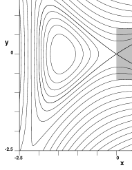
Figure 1: Level lines for potential $D_{5}$ (5) (a) and QO (6) (b). Gray color shows initial distribution of particles for $E=2E_{S}$.

The potential $D_{5}$ (5) has only two local minima and three saddles and it is the simplest potential, where the mixed state is observed.

Fig.2 presents the Poincaré sections for different energies, demonstrating evolution of dynamics in different local minima. At low energies motion has well-marked quasiperiodic character for both minima (fig.2.a,e). As energy grows, gradual regularity-to-chaos transition is observed. However changes in features of the trajectories, localized in certain minima, are sharply distinct. For the left minimum, already at about half saddle energy, significant fraction of the trajectories becomes chaotic (fig.2.b,f), and at saddle energy practically all initial conditions produce chaotic trajectories (fig.2.c,g). In right minimum under the same conditions motion remains quasiperiodic up to the saddle energy (further we will call it ”regular local minimum” for simplicity). Moreover, at energies significantly higher than the saddle energy (see fig.2), the phase space structure preserves division on chaotic and regular components (fig.2.d,h). The latter is localized in the part of the configuration space which corresponds to regular motion at energies below the saddle.

Figure 2: Poncaré surfaces of section $y=0$ in the $(x,p_{x})$ plane for the potentials $D_{5}$ (5) (a-d) and QO (6) (e-h) for different energies (from left to right): $E\lesssim E_{S}$, $E\gtrsim E_{S}$, $E=E_{S}$, $E=2E_{S}$. Solid line delimits the classically allowed region of phase space.

Earlier we have shown that the mixed state opens new possibilities for investigations of quantum signatures of classical stochasticity Berezovoj et al. (2003, 2004). Aim of the present work is to study the classical escape from separated local minima, realizing the mixed state. We show, that escape from such local minima has all the above mentioned properties of decay of chaotic systems, and also a diversity of principally new features, representing an interesting topic for conceptual understanding of chaotic dynamics, and for the applications as well. We are interested only in the ”first passage” effects, leaving aside the problem of dynamical equilibrium setup for the finite motion (for example, in $QO$ potential). In is important to stress that though we study the process of escape from a concrete local minimum, the over-barrier in the case of mixed state has a specific memory: general phase space structure at super-saddle energies is determined by the characteristics of motion in all other local minima.

We carried out numerical simulation and analytical estimates of trajectories escape in the potentials $D_{5}$ and $QO$ through the hole over the saddle point. Results of the escape problem for systems with multi-component phase volume (regular and chaotic components) essentially depend on choice of ensembles of initial conditions for dynamical variables. Fig.3 presents the normalized particle number $N(t)/N(t=0)$ for $10^{6}$ initial conditions, uniformly distributed inside the right minimum in the potential $D_{5}\ (x>0)$ and peripheral minimum in the $QO$ potential $(x>1/12)$ together with the typical trajectories and Poincare sections. The results for different potentials are evidently similar and have such characteristic features:

Figure 3: Decay law for mixed states in the $D_{5}$ (a) and $QO$ (b) potentials. Solid lines — numerical simulation for $E/E_{S}=1.1,1.5,2.0$; dotted and dashed lines — theoretically obtained exponential and linear decay laws respectively, zoomed on the inset figure in the lower left corners. Other inset figures represent the typical trajectories and Poincaré sections for the three different types of initial conditions: linearly escaping, exponentially escaping and non-escaping. Circles show the joining points between the linear and the exponential decay laws at critical time $t=\tau$.

• At times $t\rightarrow\infty$ decay law saturates at

  $$N(t\rightarrow\infty)=\rho^{(ne)}N_{0}$$

  where $\rho^{(ne)}$ is equal to relative phase volume of ”never-escaping” trajectories, which represent the regular trajectories, completely localized inside the considered minimum. All such trajectories, therefore, have infinite escaping times.

• For $t>\tau(E)$ the decay law has exponential form

  $$N(t)/N_{0}=\rho^{(ne)}+\rho^{(e)}e^{-\alpha^{(e)}(t-\tau)}$$ (7)

  where $\rho^{(e)}$ represents relative number of exponentially escaping particles.

• For $t<\tau(E)$ the decay law is linear

  $$N(t)/N_{0}=1-\alpha^{(l)}t.$$ (8)

We should stress, that (8) is in no way a linear approximation of (7) for small $t$: in general $\rho^{(ne)}+\rho^{(e)}e^{-\alpha^{(e)}\tau}\neq 1$ and $\alpha^{(e)}\rho^{(e)}e^{-\alpha^{(e)}\tau}\neq\alpha^{(l)}$. Instead, from the condition of smooth joining of curves (8) and (7) in the transition point $t=\tau$ we obtain

$$\begin{array}[]{c}\alpha^{(e)}=\alpha^{(l)}/\rho^{(e)}\\ \rho^{(e)}=1-\rho^{(ne)}-\rho^{(l)}\end{array}$$

where $\rho^{(l)}=\alpha^{(l)}\tau$ is the relative number of linearly escaping particles. Moreover, already on time scales $t\lesssim\tau(E)$ linear decay law (8) is apparently different from its exponential analogue

$$N(t)/N(t=0)=\rho^{(ne)}+(1-\rho^{(ne)})e^{(-\alpha^{(l)}t)}$$

(see the inset on fig.3).

As one can see from the inset Poincaré section on fig.3 both the chaotic and regular trajectories contribute to linear escaping regime (8), because for sufficiently small times $t<\tau$ chaotic and regular motions are not yet distinguishable. Up to transient time $t=\tau$ all quasi-one-dimensional regular trajectories, oriented along the $x$-axis, already escape and for $t>\tau$ the escape of remaining chaotic particles follows exponential law (7). The particles escaping the last show already mentioned sticking phenomenon (see the inset Poincaré sections on fig.3).

The transient time $\tau(E)$ in fact coincides with the passage time of the longest one-dimensional path from the opening to the opposite wall of the potential well and back (see fig.3). For the potentials $D_{5}$ and $QO$ corresponding theoretical estimates read (we assumed $m=1$)

$$\begin{array}[]{c}\tau_{D_{5}}(E)=2\int\limits_{0}^{\sqrt{2(1+\sqrt{E})}}\frac{dx}{|p|}=\frac{\sqrt{2}}{E^{\frac{1}{4}}}K\left(\sqrt{\frac{1+\frac{1}{\sqrt{E}}}{2}}\right)\\ \tau_{QO}(E)=12\left(\frac{E_{S}}{E}\right)^{\frac{1}{4}}K\left(\sqrt{\frac{1+\sqrt{\frac{E_{S}}{E}}}{2}}\right)=6\sqrt{2}\tau_{D_{5}}(\frac{E}{E_{S}})\end{array}$$

where $K(k)$ is the complete elliptic integral of the first kind and $E_{S}=1/12^{4}$ is the saddle energy in the $QO$ potential for $W=18$ (for the $D_{5}$ potential $E_{S}=1$).

Theoretical estimates for the escape rate were obtained by averaging the escape probability over the opening Zhao and Du (2007):

$$\alpha(E)=\rho(E)\int\limits_{x=x_{S}}dy\int\limits_{-\frac{\pi}{2}}^{\frac{\pi}{2}}d\theta|p|\cos\theta,$$

where $x_{S}$ is the coordinate of the saddle point and $\rho(E)$ is the normalized particle density:

$$\rho(E)=\frac{1}{2\pi A(E)},$$

where $A(E)$ denotes area of the classically allowed region inside the well:

$$A(E)=\int\limits_{x>x_{S}}dxdy\Theta\left(E-U(x,y)\right).$$

Such $\rho(E)$ corresponds to uniform distribution of initial conditions on the energy surface $H(\mathbf{p,q})=E$.

For the potentials $D_{5}$ and $QO$ the explicit formulae are the following:

$$A_{D_{5}}(E)=2\int\limits_{0}^{\sqrt{2(1+\sqrt{E})}}dx\sqrt{\frac{E-\left(\frac{x^{2}}{2}-1\right)^{2}}{x+2a}}$$

$$A_{QO}(E)=\frac{1}{72}\int\limits_{0}^{\sqrt{1+\sqrt{\frac{E}{E_{S}}}}}d\xi\sqrt{(\xi+4)^{2}-7}\times$$

$$\times\sqrt{\sqrt{1+\frac{\frac{E}{E_{S}}-\left(\xi^{2}-1\right)^{2}}{[(\xi+4)^{2}-7]^{2}}}-1}$$

where $\xi=\sqrt[4]{E_{S}}(x-x_{S})$.

Finally, the general expression for the escape rate is

$$\alpha(E)=\frac{\langle p\rangle}{\pi A(E)}.$$

For our case $\langle p\rangle=\int\limits_{x=x_{S}}dy|p|$. In the case of billiards with small opening $p=const\Rightarrow\langle p\rangle=p\Delta$, and we recover expression (3). For the potentials $D_{5}$ and $QO$ we get the results in closed form:

$$\alpha_{D_{5}}(E)=\frac{E-1}{2\sqrt{a}A_{D_{5}}(E)}$$

$$\alpha_{QO}(E)=\frac{\sqrt[4]{\varepsilon}}{12\pi A_{QO}(E)}\times$$

$$\times\left\{\left(16\sqrt{\varepsilon}+1\right)K\left(\sqrt{\frac{1-\frac{1}{16\sqrt{\varepsilon}}}{2}}\right)-2E\left(\sqrt{\frac{1-\frac{1}{16\sqrt{\varepsilon}}}{2}}\right)\right\}$$

where $\varepsilon=E-E_{S}+1/256$, $K(k)$ and $E(k)$ are the complete elliptic integral of the first and second kind respectively.

In order to obtain $\alpha^{(l)}(E)$ we correct $A(E)$ subtracting the relative phase space occupied by the non-escaping particles

$$A^{(l)}(E)=A(E)(1-\rho^{(ne)})\Rightarrow\alpha^{(l)}(E)=\frac{\alpha(E)}{1-\rho^{(ne)}}$$

Fig.3 demonstrates good agreement between our theoretical and numerical results for wide energy range.

Fraction of the non-escaping particles $\rho^{(ne)}$ coincides with the relative phase space volume of trajectories, localized in the regular minimum, which may be well estimated by the relative area of the stability island $\rho^{(si)}$ on the Poincaré section (fig.3). Calculation of relative area of regular island in the Poincaré section was performed by the following scheme. First, the island boundary was determined by numerical integration of equations of motion and then the interior area was calculated. Further the obtained area was divided on the entire area of classically allowed motion, defined by the conditions $x>0$ and $p^{2}>0$. While the phase volume itself is 4-dimensional, the stability island in Poincaré section is 2-dimensional, so we cannot expect absolute coincidence of the corresponding measures. However, the calculations show very close correspondence between them (see fig.4). Therefore, numerical analysis of Poincare sections together with our theoretical results gives all information necessary to predict the escape dynamics in independent way.

Figure 4: Correlations between relative area of the stability island $\rho^{(si)}(E)$ and non-escaping particles ratio $\rho^{(ne)}$: empty squares – $\rho^{(si)}_{D_{5}}(E)$, filled squares – $\rho^{(ne)}_{D_{5}}(E)$, empty circles – $\rho^{(si)}_{QO}(E)$, filled circles – $\rho^{(ne)}_{QO}(E)$.

In summary, we have considered classical escape from separated local minima in two representative $2D$ multi-well potentials, realizing the mixed state. We have found that escape from regular minima contains a number of new features. The most important among them are the following:

1. Decay law saturates at long time ranges.

2. On small time scales there exists a linear segment, which is not connected with linear approximation to the exponential decay law, observed in chaotic systems with homogeneous phase space.

3. Fraction of particles, remaining in the well, is determined by relative phase volume of the regular component, which in its turn monotonically decreases with growth of energy.

It was shown that the linear segment of the decay law is generated by the quasi-one-dimensional trajectories, oriented perpendicular to the opening, and the transient time of the linear-to-exponential regime lies in perfect agreement with the analytical estimates.

We should note that we devote main attention to escape from the regular local minima because the specifics of the mixed state manifests only in them. However let us remind that in the case of mixed state the phase space structure at super-saddle energies is determined by dynamical characteristics in different local minima of whole potential energy surface.

Above mentioned peculiarities of the escape problem may found practical application for extraction of required particle number from atomic traps. Changing energy of particles trapped inside the regular minimum, we can extract from the trap any required number of particles. Problem of particle energy changing in the potential well may be solved by introduction of small dissipation. Obtained results may present an interest also for description of induced nuclear fission in the case of double-humped fission barrier. Revealed peculiarities must manifest also in over-barrier dynamics of wave packets, initially localized in the regular minima.

V.A.Cherkaskiy was supported by grant n.50-2007 of National Academy of Science of Ukraine.

References

- Sabine (1922) W. C. Sabine, Collected Papers on Acoustics (Cambridge: Harvard Univ. Press, 1922).
- Legrand and Sornette (1990) O. Legrand and D. Sornette, Europhys. Lett. 11, 583 (1990).
- Szepfalusy and Tel (1986) P. Szepfalusy and T. Tel, Phys. Rev. A 34, 2520 (1986).
- Bauer and Bertch (1990) W. Bauer and G. F. Bertch, Phys. Rev. Lett. 65, 2213 (1990).
- Alt et al. (1996) H. Alt, H. D. Gräf, H. L. Harney, R. Hofferbert, H. Rehfeld, A. Richter, and P. Schardt, Phys. Rev. E 53(3), 2217 (1996).
- Kokshenev and Nemes (2000) V. B. Kokshenev and M. C. Nemes, Physica A 275, 70 (2000).
- Karney (1983) C. Karney, Physica D 8, 360 (1983).
- Bunimovich and Dettmann (2005) L. A. Bunimovich and C. P. Dettmann, Phys. Rev. Lett. 94, 100201 (2005).
- Milner et al. (2001) V. Milner, J. L. Hanssen, W. C. Campbell, and M. G. Raizen, Phys. Rev. Lett. 86, 1514 (2001).
- Friedman et al. (2001) N. Friedman, A. Kaplan, D. Carasso, and N. Davidson, Phys. Rev. Lett. 86, 1518 (2001).
- Zhao and Du (2007) H. J. Zhao and M. L. Du, Phys. Rev. E 76, 027201 (2007).
- Bolotin et al. (1987) Y. L. Bolotin, V. Y. Gonchar, and E. V. Inopin, Yad.Fiz. 45, 350 (1987).
- Gilmor (1981) R. Gilmor, Catastrophe Theory (New-York: Wiley, 1981).
- Mozel and Greiner (1968) V. Mozel and W. Greiner, Z. Phys A. 217(3), 256 (1968).
- Berezovoj et al. (2003) V. P. Berezovoj, Y. L. Bolotin, and V. A. Cherkaskiy, Prog. Theor. Phys. Supplement 150, 326 (2003).
- Berezovoj et al. (2004) V. P. Berezovoj, Y. L. Bolotin, and V. A. Cherkaskiy, Phys. Lett. A 323, 218 (2004).