Hidden Life of
Riemann’s Zeta Function
2. Electrons and Trains

Abstract

The Riemann Hypothesis can be reformulated as statements about the eigenvalues of certain matrices whose entries are defined in terms of the Taylor coefficients of the zeta function. These eigenvalues exhibit interesting visual patterns allowing one to state a number of conjectures.

The Hankel matrices introduced here are obtained, by rearranging of columns, from Toeplitz matrices whose eigenvalues were considered in http://arXiv.org/abs/0707.1983. The present paper is a continuation of this paper and references such as 1X, 1.x, (1.x.y), and 1.x.y refer respectively to conjectures, sections, formulas, or figures from there.

2.1 Hankel matrix representation

As it was indicated in Section 1.6, we can give an alternative representation for the numbers $\tau_{m}$ (defined by the expansion (1.5.1)), in the form of determinants, by rearranging the columns of the matrices $L_{1,m}$ introduced by (1.6.3). More generally, we rearrange the columns of the matrices $L_{l,m}(f)$ defined by (1.14.2):

$$M_{l,m}(f)=$$ (2.1.1)

$$-(-1)^{\frac{(m+1)(m+2)}{2}}\begin{pmatrix}\theta_{l+m-1}(f)&\theta_{l+m-2}(f)&\dots&\theta_{l}(f)\\ \theta_{l+m-2}(f)&\theta_{l+m-3}(f)&\dots&\theta_{l-1}(f)\\ \vdots&\vdots&\ddots&\vdots\\ \theta_{l}(f)&\theta_{l-1}(f)&\dots&\theta_{l-m+1}(f)\end{pmatrix}.$$

Clearly, for all $l$ and $m$ we have

$$\det(M_{l,m}(f))=\det(L_{l,m}(f)),$$ (2.1.2)

so we have the following reformulations of versions 2 and 3 of subhypothesis ${\mathrm{RH}}_{l}^{\mathrm{w}}$ from Sections 1.14 (with ${\mathrm{W}}_{l}$ defined by (1.12.10)):

$\mathbf{RH_{\emph{l}}^{w}}$ (version $\mathbf{2}^{\prime}$). For $m\rightarrow\infty$

$$\det(M_{l,m}({\zeta^{*}}))\,=\,{\mathrm{W}}_{l}^{m}({\mathrm{R}}_{l}({\zeta^{*}})+o(1)).$$ (2.1.3)

with some constant ${\mathrm{R}}_{l}({\zeta^{*}})$.

$\mathbf{RH_{\emph{l}}^{w}}$ (version $\mathbf{3}^{\prime}$).

$$\lim_{m\rightarrow\infty}\left(\det(M_{l,m}({\zeta^{*}}))\right)^{\frac{1}{m}}\,=\,{\mathrm{W}}_{l}.$$ (2.1.4)

2.2 Yet More Eigenvalues

By analogy with (1.15.1), we have the representation

$$\det(M_{l,m}(f))=\mu_{l,m,1}(f)\mu_{l,m,2}(f)\dots\mu_{l,m,m}(f)$$ (2.2.1)

where $\mu_{l,m,1}(f),\ \mu_{l,m,2}(f),\ \dots,\ \mu_{l,m,m}(f)$ are the eigenvalues of the matrix $M_{l,m}(f)$. Respectively, we have

$\mathbf{RH_{\emph{l}}^{w}}$ (version 5).

$$\lim_{m\rightarrow\infty}\left(\prod_{n=1}^{m}{\mu_{l,m,n}({\zeta^{*}})}\right)^{\frac{1}{m}}={\mathrm{W}}_{l}.$$ (2.2.2)

The (multi)set $\{\mu_{l,m,1}(f),\ \mu_{l,m,2}(f),\dots\mu_{l,m,m}(f)\}$ will be called $\mu$-spectrum of the function $f$ and will be denoted ${\mathrm{Spec}}^{\mu}_{l,m}(f)$.

2.3 Positions of the $\mu$ eigenvalues

According to (2.2.2), the (geometric) mean of $\mu_{1,m,1}({\zeta^{*}})$, $\mu_{1,m,2}({\zeta^{*}})$, …, $\mu_{1,m,m}({\zeta^{*}})$ approaches ${\mathrm{W}}_{l}$ when $m$ goes to infinity, which is similar to the behavior of the eigenvalues $\lambda_{1,m,1}({\zeta^{*}})$, $\lambda_{1,m,2}({\zeta^{*}})$, …, $\lambda_{1,m,m}({\zeta^{*}})$. However, there are many differences between the distribution of the eigenvalues from spectra ${\mathrm{Spec}}^{\mu}_{l,m}({\zeta^{*}})$ and ${\mathrm{Spec}}^{\lambda}_{l,m}({\zeta^{*}})$.

The first such difference is evident: the numbers $\mu_{1,m,1}({\zeta^{*}})$, $\mu_{1,m,2}({\zeta^{*}})$, …, $\mu_{1,m,m}({\zeta^{*}})$, being the eigenvalues of a Hankel matrix with real entries, are all real themselves.

Computations suggest that in contrast to the case of the $\lambda$-spectra, the union $\cup_{m=1}^{\infty}{\mathrm{Spec}}^{\mu}_{l,m}({\zeta^{*}})$ is bounded neither from above nor from below. Moreover, the point $0$ is a limit point of this set. That is why it is reasonable to consider the sets

$${\mathrm{Spec}}^{\ln|{\mu}|}_{l,m}(f)=\{\ln|\mu|:\mu\in{\mathrm{Spec}}^{\mu}_{l,m}(f)\}$$ (2.3.1)

which will be called logarithmic $\mu$-spectra. When exhibiting several logarithmic $\mu$-spectra, we will shift the lines vertically, that is, an eigenvalue $\ln|\mu|$ from ${\mathrm{Spec}}^{\ln|{\mu}|}_{l,m}(f)$ will be placed at point $(x,y)=(\ln|\mu|,m)$.

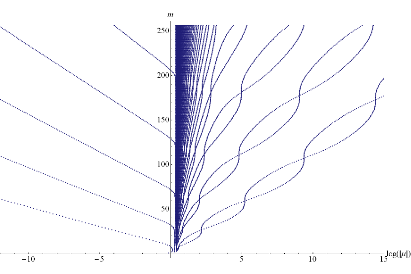
Figure 2.3.1: ${\mathrm{Spec}}^{\ln|{\mu}|}_{1,m}({\zeta^{*}}),\ m=1,\dots,256.$

Figure 2.3.2: ${\mathrm{Spec}}^{\ln|{\mu}|}_{2,m}({\zeta^{*}}),\ m=1,\dots,256.$

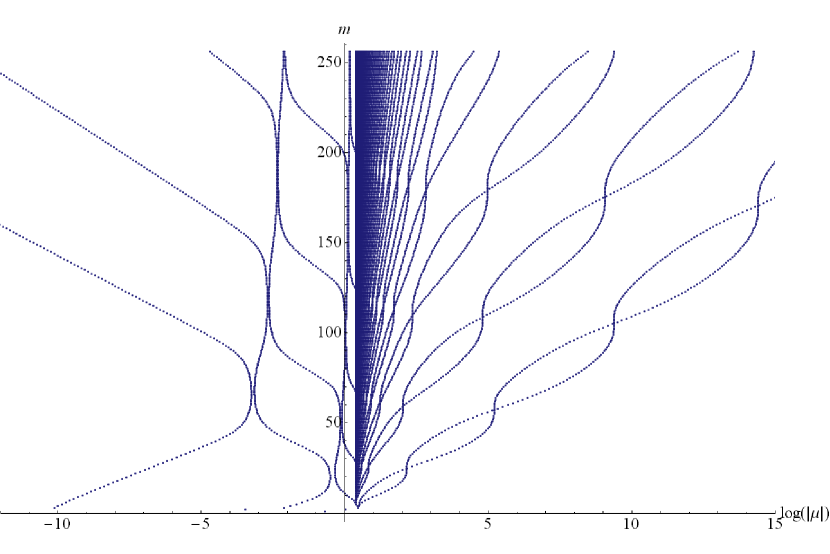
Figure 2.3.3: ${\mathrm{Spec}}^{\ln|{\mu}|}_{3,m}({\zeta^{*}}),\ m=1,\dots,256.$

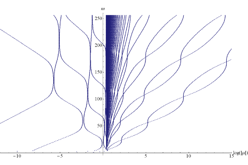
Figure 2.3.4: ${\mathrm{Spec}}^{\ln|{\mu}|}_{4,m}({\zeta^{*}}),\ m=1,\dots,256.$

Figure 2.3.5: ${\mathrm{Spec}}^{\ln|{\mu}|}_{5,m}({\zeta^{*}}),\ m=1,\dots,256.$

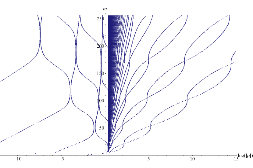
Figure 2.3.6: ${\mathrm{Spec}}^{\ln|{\mu}|}_{6,m}({\zeta^{*}}),\ m=1,\dots,256.$

Figures 2.3.1–2.3.6 show spectra ${\mathrm{Spec}}^{\ln|{\mu}|}_{1,m}({\zeta^{*}})$, …, ${\mathrm{Spec}}^{\ln|{\mu}|}_{2,m}({\zeta^{*}})$ for $m=1,\dots,256$ (higher resolution version of these pictures can be downloaded from [1] as well as some animations showing these spectra and thus revealing another kind of “hidden life of Riemann’s zeta function”).

The pictures and the animations show that with the growth of $m$ some elements of ${\mathrm{Spec}}^{\ln|{\mu}|}_{l,m}({\zeta^{*}})$ go to $-\infty$ while others go to $+\infty$; the former will be called electrons and the latter will be called trains (we postpone formal definition of splitting ${\mathrm{Spec}}^{\ln|{\mu}|}_{l,m}({\zeta^{*}})$ into lower part ${\mathrm{Spec}}^{\ln|{\mu}|<}_{l,m}({\zeta^{*}})$, consisting of the electrons, and upper part ${\mathrm{Spec}}^{\ln|{\mu}|>}_{l,m}({\zeta^{*}})$ consisting of the trains).

The names “electrons” and “trains” were suggested by the following visual patterns. The electrons behave like charged particles, namely, they bounce. The trains all go in pairs (a surprising feature!) and every now and then they overtake one another.

2.4 New Conjectures

The above pictures suggest the following conjectures.

Conjecture 2A. For all $l$

$$\lim_{m\rightarrow\infty}\max({\mathrm{Spec}}^{\ln|{\mu}|}_{l,m}({\zeta^{*}}))=+\infty.$$ (2.4.1)

Conjecture 2B. For all $l$

$$\lim_{m\rightarrow\infty}\min({\mathrm{Spec}}^{\ln|{\mu}|}_{l,m}({\zeta^{*}}))=-\infty.$$ (2.4.2)

It is impossible to see from the above pictures whether for the $\mu$-spectra there is a counterpart of Conjecture 1F about the $\lambda$-spectra. To make this clearer, in analogy with this conjecture, let us assign to each point of ${\mathrm{Spec}}^{\ln|{\mu}|}_{l,m}({\zeta^{*}})$ the weight $\frac{1}{m}$, and denote by $\mu^{{\zeta^{*}}}_{l,m}(x)$ the corresponding discrete measure on real numbers. Further, let $F^{{\zeta^{*}}}_{l,m}(x)$ denote the corresponding distribution function. In terms of these functions we have

$\mathbf{RH_{\emph{l}}^{w}}$ (version 6).

$$\lim_{m\rightarrow\infty}\left(\int_{-\infty}^{+\infty}x\,{\mathrm{d}}F^{{\zeta^{*}}}_{l,m}(x)\right)=\log({\mathrm{W}}_{l}).$$ (2.4.3)

Figure 2.4.1: $F^{{\zeta^{*}}}_{1,8}(x).$

Figure 2.4.2: $F^{{\zeta^{*}}}_{1,16}(x).$

Figure 2.4.3: $F^{{\zeta^{*}}}_{1,32}(x).$

Figure 2.4.4: $F^{{\zeta^{*}}}_{1,64}(x).$

Figure 2.4.5: $F^{{\zeta^{*}}}_{1,128}(x).$

Figure 2.4.6: $F^{{\zeta^{*}}}_{1,256}(x).$

Figure 2.4.7: $F^{{\zeta^{*}}}_{6,8}(x).$

Figure 2.4.8: $F^{{\zeta^{*}}}_{6,16}(x).$

Figure 2.4.9: $F^{{\zeta^{*}}}_{6,32}(x).$

Figure 2.4.10: $F^{{\zeta^{*}}}_{6,64}(x).$

Figure 2.4.11: $F^{{\zeta^{*}}}_{6,128}(x).$

Figure 2.4.12: $F^{{\zeta^{*}}}_{6,256}(x).$

Figures 2.4.2–2.4.12 show these functions for $l=1,6$ and $m=8,16,32,64,256$. These pictures suggest

Conjecture 2C. For every $l$ functions $F^{{\zeta^{*}}}_{l,m}(x)$ have, as $m\rightarrow\infty$, the pointwise limiting continuous distribution function $F_{l}^{{\zeta^{*}}}\!(x)$.

This is an analog of part $\mathrm{1F^{\prime}}$ of Conjecture 1F for $\lambda$-spectra. However, it seems that part $\mathrm{1F^{\prime\prime}}$ of this conjecture has no analog for $\mu$-spectra. According to (2.4.3), such an analog would say that for all $l$

$$\int_{-\infty}^{+\infty}x\,{\mathrm{d}}F^{{\zeta^{*}}}_{l}(x)=\log({\mathrm{W}}_{l}).$$ (2.4.4)

But theses integrals do not seem to exist:

Conjecture 2D. For every $l$

$$\int_{-\infty}^{0}x\,{\mathrm{d}}F^{{\zeta^{*}}}_{l}(x)=-\infty, \int_{0}^{+\infty}x\,{\mathrm{d}}F^{{\zeta^{*}}}_{l}(x)=+\infty.$$ (2.4.5)

This implies that the validity of (2.4.3) should be due to some fine correlation between eigenvalues from ${\mathrm{Spec}}^{\ln|{\mu}|<}_{l,m}({\zeta^{*}})$ and ${\mathrm{Spec}}^{\ln|{\mu}|>}_{l,m}({\zeta^{*}})$. The subtleness of this correlation follows from (very surprising)

Conjecture 2E. All distribution functions $F^{{\zeta^{*}}}_{l}(x)$ coincide; that is, for all $l$ and $x$

$$F^{{\zeta^{*}}}_{l}(x)=F^{{\zeta^{*}}}(x)$$ (2.4.6)

for some continuous distribution function $F^{{\zeta^{*}}}(x)$.