LHC Signals for Warped Electroweak Neutral Gauge Bosons

Abstract

We study signals at the Large Hadron Collider (LHC) for Kaluza-Klein (KK) excitations of the electroweak gauge bosons in the framework with the Standard Model (SM) gauge and fermion fields propagating in a warped extra dimension. Such a framework addresses both the Planck-weak and flavor hierarchy problems of the SM. Unlike the often studied $Z^{\prime}$ cases, in this framework, there are three neutral gauge bosons due to the underlying $SU(2)_{L}\times SU(2)_{R}\times U(1)_{X}$ gauge group in the bulk. Furthermore, couplings of these KK states to light quarks and leptons are suppressed, whereas those to top and bottom quarks are enhanced compared to the SM gauge couplings. Therefore, the production of light quark and lepton states is suppressed relative to other beyond the SM constructions, and the fermionic decays of these states are dominated by the top and bottom quarks, which are, though, overwhelmed by KK gluons dominantly decaying into them. However, as we emphasize in this paper, decays of these states to longitudinal $W$, $Z$ and Higgs are also enhanced similarly to the case of top and bottom quarks. We show that the $W$, $Z$ and Higgs final states can give significant sensitivity at the LHC to $\sim 2\;(3)$ TeV KK scale with an integrated luminosity of $\sim 100$ fb^-1 ($\sim 1$ ab^-1). Since current theoretical framework(s) favor KK masses $\gtrsim 3$ TeV, luminosity upgrade of LHC is likely to be crucial in observing these states.

1 Introduction

The hierarchy between the Planck scale and the electroweak (EW) scales has been one of the deep mysteries of the Standard Model (SM) for the past couple of decades. Solutions to this hierarchy problem invoke new physics at the weak or TeV scale. Hence, the upcoming Large Hadron Collider (LHC) with center of mass energy of $14$ TeV has the potential to test such ideas. In this paper, we focus on one such solution based on the Randall-Sundrum (RS1) framework of a warped extra dimension [1]. Specifically, we consider this framework with the SM fermion and gauge fields propagating in the extra dimension (or “bulk”). Such a scenario can also explain the hierarchy between the SM fermion masses and mixing angles (flavor hierarchy). Moreover, in this framework, there are Kaluza-Klein (KK) excitations of the SM gauge and fermionic fields with mass at the TeV scale, leading to potential signals from these new states at the LHC. In particular, the prospects for detection of the KK gluon have been studied recently [2], and references [3] studied signals for the KK graviton in this scenario.

As a next step in this program, here we study signals from KK modes of the EW gauge bosons, focusing on the neutral ones in this paper. Just like the case of the KK gluon, the fermionic decay modes of the EW KK states are dominated by the top (and in some cases bottom) quarks, in particular, the decays to the “golden” leptonic channels tend to be suppressed unlike the $Z^{\prime}$’s studied extensively in the literature. However, as we discuss in this paper, a new feature for EW states (with respect to the KK gluon) is enhanced decays (comparable to that into top quarks) of EW KK states into longitudinal $W$, $Z$ and Higgs. We therefore focus on the $W$, $Z$ and Higgs final states since the decays to top and bottom final states are overwhelmed by decays of the KK gluon which dominantly decay into them. In addition, there are multiple EW KK states (namely 3 for neutral and 2 for charged) which mix with each other, resulting in interesting phenomenology and decay patterns. We find that the LHC with $\sim 100$ fb^-1 to $\sim 1$ ab^-1 luminosity can be sensitive to masses for EW states in the $2$ to $3$ TeV range using the $W$, $Z$ and Higgs final states, smaller than in the cases of KK gluon due to the larger cross-section for the latter. However, as we will discuss in next section, KK masses $\gtrsim 3$ TeV are preferred by precision electroweak and flavor tests for the simplest existing models in the literature. So, our results provide a strong motivation for LHC upgrade.

The paper is organized as follows. In Sec. 2, we briefly review the basic setting in the warped extra dimension scenario focusing on the electroweak gauge bosons, and in Sec. 3 present details on the different neutral states in the theory. We calculate the widths and branching fractions for their decays in Sec. 4. In Sec. 5 we give the main results of our paper. Here, we consider various signals based on these couplings, focusing on decays of the neutral modes to $W^{+}W^{-}$, $Z\,h$ and $l^{+}l^{-}$ (even though the latter channel is suppressed, it can be important due to its cleanness). We defer a study of charged EW states to a future publication. In appendices A and B we present in detail the couplings of these heavy EW gauge bosons to the SM fermions and the SM gauge bosons – in particular, we present a derivation of couplings of heavy EW gauge bosons to the SM gauge bosons, and the corresponding Feynman rules of the couplings of the KK gauge bosons to the SM fields.

2 Warped Extra Dimension: Lay of the Land

2.1 Original RS1

The framework is based on a slice of AdS₅. Owing to the warped geometry, the relationship between the $5D$ mass scales (taken to be of order $4D$ reduced Planck scale, ${\bar{M}}_{P}$) and those in an effective $4D$ description depends on the location in the extra dimension. The $4D$ (or zero-mode) graviton is localized near the “UV/Planck” brane which has a Planckian fundamental scale, whereas the Higgs sector is localized near the “IR/TeV” brane where it is stable near a warped-down fundamental scale of order TeV. The crucial point is that this large hierarchy of scales can be generated via a modest-sized radius of the $5^{\rm th}$ dimension: $\hbox{TeV}/{\bar{M}}_{P}\sim e^{-k\pi r_{c}}$, where $k$ is the curvature scale and $R$ is the proper size of the extra dimension; $kR\approx 11$. Furthermore, such a size of the extra dimension can be stabilized by suitable mechanisms [4]. Finally, based on the AdS/CFT correspondence [5], RS1 is conjectured to be dual to $4D$ composite Higgs models [6, 7, 8].

In the original RS1 model, the entire SM (including the fermions and gauge bosons) are assumed to be localized on the TeV brane. The key feature of this model is that the only new particles are the KK gravitons with no SM gauge quantum numbers (color/electroweak charge). These KK gravitons have a mass $\sim$ TeV and are localized near the TeV brane so that KK graviton coupling to the entire SM is only $\sim$ TeV suppressed. Hence, KK graviton production via $q\bar{q}$ or $gg$ fusion at the LHC [or via $e^{+}e^{-}$ at International Linear Collider (ILC)] followed by decays to dileptons or diphotons gives striking signals [9].

2.2 SM in bulk

However, it was subsequently realized that to solve the Planck-weak hierarchy problem only the SM Higgs boson has to be localized on/near the TeV brane – the rest of the SM (fermion and gauge fields) can be allowed to propagate in the extra dimension [10, 11, 12] since their masses are protected by gauge and chiral symmetries. Moreover, such a scenario enables a solution to the following problem of the original RS1 model. Namely, the higher-dimensional operators in the $5D$ effective field theory (from physics at the cut-off) are suppressed only by the warped-down cut-off $\sim$ TeV [assuming $O(1)$ coefficients for these operators], giving too large contributions to flavor changing neutral current (FCNC) processes and observables related to SM electroweak precision tests (EWPT). The point is that in this new scenario (with the SM in the bulk) the SM particles are identified with the zero-modes of the $5D$ fields and the profile of a SM fermion in the extra dimension depends on its $5D$ mass parameter. We can then choose to localize 1st and 2nd generation fermions near the Planck brane so that the FCNC’s from higher-dimensional operators are suppressed by scales $\gg$ TeV which is the cut-off at the location of these fermions [12, 13]. Similarly, contributions to EWPT from cut-off physics are also suppressed.

As a further bonus, we obtain a solution to the flavor puzzle in the sense that hierarchies in the SM Yukawa couplings arise without introducing hierarchies in the fundamental $5D$ theory [11, 12, 13]: the 1st/2nd generation fermions have small Yukawa couplings to Higgs which is localized near the TeV brane. Similarly, the top quark can be localized near the TeV brane to account for its large Yukawa coupling.

In this framework, there are KK excitations of SM gauge and fermion fields in addition to those of the graviton. These states have mass in the TeV range and are localized near the TeV brane (just like KK gravitons). Hence, we obtain new possibilities for collider signals, but at the same time, there are new contributions to FCNC’s and EWPT which are calculable in the $5D$ effective field theory (EFT). However, due to various symmetries (approximate flavor or analog of GIM mechanism of the SM [12, 13, 14] and custodial isospin [15]), we can show that gauge KK masses as small as $\sim 3$ TeV are consistent with oblique electroweak (EW) data [15] (we comment on non-oblique effects such as $Zb\bar{b}$ below) and FCNC’s [16].

Let us consider the top and bottom sector in detail to determine the couplings to KK states. Due to heaviness of top quark combined with constraint from shift in $Zb\bar{b}$, one possibility is to localize $t_{R}$ very close to TeV brane with $(t,b)_{L}$ having a profile close to flat [15]. Even with this choice of the profiles, the gauge KK mass scale is constrained by $Zb\bar{b}$ to be $\stackrel{{\scriptstyle>}}{{\sim}}5$ TeV [21, 22], i.e., a bit higher than that allowed by oblique EW data. However, a custodial symmetry to suppress $Zb\bar{b}$ [23] can relax this constraint on the gauge KK mass scale and moreover allows even the other extreme case: $(t,b)_{L}$ very close to the TeV brane and $t_{R}$ close to flat and also the intermediate possibility with both $t_{R}$ and $(t,b)_{L}$ being near, but not too close to TeV brane [21, 24, 25, 26]. The bottom-line is that, with this custodial symmetry for $Zb\bar{b}$ and for certain choices of profiles for $t_{R}$ and $(t,b)_{L}$ in the extra dimension, gauge KK masses as low as $\sim 3$ TeV can be consistent with $Zb\bar{b}$ as well.

Clearly, couplings of gauge KK modes to light fermions (to top and bottom) are suppressed (enhanced) compared to the SM gauge coupling simply based on the overlap of the corresponding profiles in the extra dimension (the zero-mode or SM gauge boson has a flat profile in the extra dimension). As a consequence, production of the gauge KK modes tends to be suppressed compared to the $Z^{\prime}/W^{\prime}$’s often studied in the literature. Moreover, their fermionic decay modes are dominated by top and bottom quarks (which are not easily detectable modes). In spite of these difficulties, it was shown in references [2] that the LHC can be sensitive to KK gluon masses up to $\sim 4$ TeV based on decays to top quarks.

2.3 EW gauge states

However, for EW KK modes, there is a possibility of sizable decays to cleaner final states (compared to the KK gluon) as follows. The crucial point being that by the equivalence theorem, longitudinal $W$ and $Z$ (denoted by $W^{\pm}_{L}$ and $Z_{L}$) are effectively the unphysical Higgs (“would-be” Goldstone bosons) and are therefore localized near TeV brane (just like the physical Higgs). So, the decay widths for EW KK states in the $W_{L}/Z_{L}$ channels are the same size as in those of the physical Higgs/top quark. Clearly, branching ratio of EW KK states to a pair of $Z/W$’s is sizable; in particular, $Z_{L}Z_{L}$ is not allowed (it is for KK graviton!), but $WW$, $ZW$, $Zh$ and $Wh$ are good decay channels. As a corollary, production of EW KK states via longitudinal $W$ and $Z$ fusion (weak boson fusion, WBF) can be potentially important. Such effects were not analyzed before in this class of models, including in the recent paper [27] which focuses on decays to top and bottom final states. However, the signal from electroweak neutral states in top/bottom final state is likely to be swamped by the KK gluon which dominantly decays to this final state with a coupling larger than that for the case of EW KK states. Our motivation is to study the heavy electroweak gauge bosons and hence we consider their decays to the top/bottom final state only in passing and focus on the $W/Z/$Higgs final state instead. To summarize, the relevant coupling to the KK gauge states can be described schematically (see section A for more details), neglecting effects related to EWSB, via ratio of RS1-to-SM gauge coupling

$${g_{\rm RS}^{q\bar{q},l\bar{l}\,Z_{KK}^{(1)}}\over g_{\rm SM}} \simeq -\xi^{-1}\approx-{1\over 5}$$

$${g_{\rm RS}^{Q_{3}\bar{Q}_{3}Z_{KK}^{(1)}}\over g_{\rm SM}},\ \ {g_{\rm RS}^{t_{R}\bar{t}_{R}Z_{KK}^{(1)}}\over g_{\rm SM}} \simeq 1\;\hbox{to}\;\xi\;(\approx 5)$$

$${g_{\rm RS}^{HHZ_{KK}^{(1)}}\over g_{\rm SM}} \simeq \xi\approx 5\;\;\;\left(H=h,W_{L},Z_{L}\right)$$ (1)

where $q=u,d,s,c,b_{R}$, $l=$ all leptons, $Q^{3}=(t,b)_{L}$, $Z_{KK}^{(1)}$ represents the first KK state of the gauge fields (in the KK-basis), $g_{\rm RS}^{xyz},g_{\rm SM}$ stands for the RS KK mode and the three SM (i.e., $4D$) gauge couplings respectively, and $\xi\equiv\sqrt{k\pi r_{c}}$ (cf Eq. (36)). Also, $H$ includes both the physical Higgs ($h$) and longitudinal $W$ and $Z$. EWSB induces mixing between EW KK states which we discuss in what follows.

3 Summary and overview of the electroweak gauge sector

Here we give a summary of the various EW gauge bosons present in the model and refer the reader to the appendices for details of their properties. The electroweak gauge group in the bulk is $SU(2)_{L}\times SU(2)_{R}\times U(1)_{X}$. So, we have 3 electrically neutral towers from the $U(1)_{L,R,X}$ gauge sectors. The $U(1)_{R,X}$ towers mix via the boundary condition on the Planck brane, and the Higgs vev which couples to $U(1)_{L,R}$ mixes these towers further. The Higgs is localized near the TeV brane.

We will find it convenient to rewrite and reorganize the neutral towers into towers of photon, $Z$ (same combinations as in the SM) and $Z_{X}$ – which is the combination of $U(1)_{R,\;X}$ orthogonal to $U(1)_{Y}$ – towers. Before turning on the Higgs vev, zero-modes are present only in the photon and $Z$ towers. Even after EWSB, the photon tower does not mix with the other two towers nor do the various modes (both zero and KK) of this tower mix with each other – the zero-mode photon is then identified with the SM photon. The $Z$ and $Z_{X}$ towers do mix via the Higgs vev – specifically, the zero-mode $Z$ mixes with KK modes from both towers and the KK modes of the two towers mix with each other as well (cf Eqs. (61), (82) and (83)). The lightest mode of the resulting mixtures is the SM $Z$. We will discuss the phenomenology of only the 1st KK mode in each tower (for simplicity and also because the effects of heavier KK modes is suppressed) denoting it by $A_{1}$, $Z_{1}$ and ${Z_{X}}_{1}$ respectively in the KK basis, and as $A_{1}$, $\tilde{Z}_{1}$ and $\tilde{Z}_{X1}$ for the mass basis eigenstates, collectively referring to these mass eigenstates as ${Z^{\prime}}$.

Similarly, there are 2 charged towers corresponding to $W_{L}^{\pm}$ and $W_{R}^{\pm}$ – only the former tower has a zero-mode. Due to Higgs vev, these two towers mix just like for the neutral sector and the resulting lightest mode is the SM $W$ (cf Eqs. (47) (84) and (85)).

As explained above, the heavy gauge bosons will decay mostly to longitudinal $WW$, longitudinal $Zh$, $t\bar{t}$ and $b\bar{b}$ since the couplings to these final states are in fact enhanced relative to the SM, whereas the couplings to leptons and light quarks are suppressed relative to the SM (see Eq. (1)). As mentioned above, there are various possibilities for quantum numbers of the top and bottom quarks and their profiles in the extra dimension (for details see Secs. A.3 and A.4). For the analysis in this paper, we will choose $(t,b)_{L}$ to be a doublet of $SU(2)_{R}$ with an approximately flat profile – the motivation being to suppress corrections to $Zb_{L}\bar{b}_{L}$ and flavor violation, with $t_{R}$ being a singlet or triplet of $SU(2)_{R}$ and localized near the TeV brane. It is possible to obtain a good fit to the precision electroweak data (in particular $T$ parameter can be positive and of the required size) for such a choice of parameters [21].

Having made this choice for top and bottom quarks, we would like to mention that our focus in this paper is on the production of the heavy electroweak gauge bosons via quarks in the initial state followed by decays to $WW$, $Zh$ final states. The total production cross-section of the heavy gauge bosons and the partial decay widths to these final states are not affected significantly by the choice of top and bottom profiles and representations. The partial decay widths to $t\bar{t}$ and $b\bar{b}$ and so the total width and, in turn, the production cross-section for specific final states are of course affected by the choice of representation and profile of the top and bottom quarks, but not by more than an $O(1)$ factor.

Figure 1: The total width of ${Z^{\prime}}$ as a function of its mass.

4 ${Z^{\prime}}$ decays

The decay widths for the leading channels of the neutral KK gauge bosons, which are generically denoted by ${Z^{\prime}}$ unless specified otherwise, are given by

$$\Gamma(A_{1}\rightarrow W_{L}W_{L}) = \frac{e^{2}\kappa^{2}}{192\pi}\frac{M_{Z^{\prime}}^{5}}{m_{W}^{4}}\ ;\ \ \ \ \kappa\propto\sqrt{k\pi r_{c}}\left(\frac{m_{W}}{M_{W^{\pm}_{1}}}\right)^{2}\ ,$$ (2)

$$\Gamma(\tilde{Z}_{1},\tilde{Z}_{X1}\rightarrow W_{L}W_{L}) = \frac{g_{L}^{2}c_{W}^{2}\kappa^{2}}{192\pi}\frac{M_{Z^{\prime}}^{5}}{m_{W}^{4}}\ ;\ \ \ \ \kappa\propto\sqrt{k\pi r_{c}}\left(\frac{m_{Z}}{(M_{Z_{1}},M_{{Z_{X}}_{1}})}\right)^{2}\ ,$$ (3)

$$\Gamma(\tilde{Z}_{1},\tilde{Z}_{X1}\rightarrow Z_{L}h) = \frac{g_{Z}^{2}\kappa^{2}}{192\pi}M_{Z^{\prime}}\ ;\ \ \ \ \kappa\propto\sqrt{k\pi r_{c}}\ ,$$ (4)

$$\Gamma({Z^{\prime}}\rightarrow f\bar{f}) = \frac{(e^{2},g_{Z}^{2})}{12\pi}\left(\kappa_{V}^{2}+\kappa_{A}^{2}\right)M_{Z^{\prime}}\ ,$$ (5)

where for a quark final state the appropriate color factor (3) should be included (which has not been included above), and $\sqrt{k\pi r_{c}}=\xi$ as described in Sec. A.1.1. $\kappa$ is the coupling of the ${Z^{\prime}}$ to the respective final states relative to that of the corresponding SM coupling. The fermion couplings have been defined such that the coefficient of $\gamma_{\mu}$ is $g_{Z}\kappa_{V}$ and that of $\gamma_{\mu}\gamma_{5}$ is $g_{Z}\kappa_{A}$ (the $\kappa$ along with the SM factors are given in Table 9 via $\kappa_{V}=(\kappa_{R}+\kappa_{L})/2,\ \kappa_{A}=(\kappa_{R}-\kappa_{L})/2$ ). Since $A_{1}$ is the KK excitation of the photon, the physical Higgs modes are not available for it to decay into. Next to the equations above, the order of magnitude of $\kappa$ is shown without the $(Z_{1},{Z_{X}}_{1})$ mixing factors. Including these mixing factors, the $\kappa$ are more accurately written as

$$\kappa_{A_{1}WW} = -2s_{0L}\ ,$$ (6)

$$\kappa_{\tilde{Z}_{1}WW} = s_{01}c_{1}-s_{01X}s_{1}-2c_{1}s_{0L}\ ,$$ (7)

$$\kappa_{\tilde{Z}_{X1}WW} = s_{01}s_{1}+s_{01X}c_{1}-2s_{1}s_{0L}\ ,$$ (8)

$$\kappa_{\tilde{Z}_{1}Zh} = \sqrt{k\pi r_{c}}(c_{1}+\frac{g_{R}}{g_{L}}c_{W}c^{\prime}s_{1})\ ,$$ (9)

$$\kappa_{\tilde{Z}_{X1}Zh} = \sqrt{k\pi r_{c}}(s_{1}-\frac{g_{R}}{g_{L}}c_{W}c^{\prime}c_{1})\ .$$ (10)

where $s_{01}$ is the (sine of the) $Z^{(0)}\leftrightarrow Z_{1}$ mixing angle where $Z^{(0)}$ is the $Z$ zero-mode, $s_{01X}$ that of $Z^{(0)}\leftrightarrow{Z_{X}}_{1}$, $s_{1}$ that of $Z_{1}\leftrightarrow{Z_{X}}_{1}$ and $s_{0L}$ that of $W^{(0)}\leftrightarrow W_{L_{1}}$. As explained in Sec. 3, expressions for these mixing angles are given in Apps. A and B.

Figure 2: The branching ratios of ${Z^{\prime}}$ into the various modes as a function of its mass for $A_{1}$ (left), $\tilde{Z}_{1}$ (center) and $\tilde{Z}_{X_{1}}$ (right).

In Fig. 1 we show the decay width as a function of $M_{Z^{\prime}}$. In our numerical study we set $g_{R}=g_{L}\approx g$, the SM $SU(2)_{L}$ coupling. We base our numerical study of the decay widths and BR’s on the analytical calculations presented above, with some checks performed using the program BRIDGE [29]. The widths are all linearly proportional to the mass after properly taking into account the mixings in the couplings, being about $5\%$ of its mass and thus remain relatively narrow. In Fig. 2 we show the ${Z^{\prime}}$ branching ratios into the various modes of our current interests. We see that for $A_{1}$, all channels have the trivial mass dependence. There is no $Zh$ channel, and the two leading channels $t\bar{t}$ and $WW$ are comparable. For $\tilde{Z}_{1}$, the leading channel is $Zh$ and the next is $t\bar{t}$. The suppressed coupling to $WW$ can be understood from the equivalence theorem – for the mass range shown it happens that the eaten charged Goldstone boson almost decouples from this state. A similar argument, but for the eaten neutral Goldstone boson explains the suppression of the $Zh$ mode in the case of $\tilde{Z}_{X1}$. In all cases, the charged lepton mode $\ell\ell$ is very small, ranging in $10^{-3}-10^{-4}$. As a representative, in Table 1 we show the partial widths and the decay branching ratios for $M_{Z^{\prime}}=2$ TeV.

Table 1: Partial widths and decay branching ratios for $M_{Z^{\prime}}=2$ TeV.

	$A_{1}$		$\tilde{Z}_{1}$		$\tilde{Z}_{X1}$
	$\Gamma$(GeV)	BR	$\Gamma$(GeV)	BR	$\Gamma$(GeV)	BR
$\bar{t}t$	$55.8$	$0.54$	$18.3$	$0.16$	$55.6$	$0.41$
$\bar{b}b$	$0.9$	$8.7\times 10^{-3}$	$0.12$	$10^{-3}$	$28.5$	$0.21$
$\bar{u}u$	$0.28$	$2.7\times 10^{-3}$	$0.2$	$1.7\times 10^{-3}$	$0.05$	$4\times 10^{-4}$
$\bar{d}d$	$0.07$	$6.7\times 10^{-4}$	$0.25$	$2.2\times 10^{-3}$	$0.07$	$5.2\times 10^{-4}$
$\ell^{+}\ell^{-}$	$0.21$	$2\times 10^{-3}$	$0.06$	$5\times 10^{-4}$	$0.02$	$1.2\times 10^{-4}$
$W_{L}^{+}W_{L}^{-}$	$45.5$	$0.44$	$0.88$	$7.7\times 10^{-3}$	$50.2$	$0.37$
$Z_{L}h$	-	-	$94$	$0.82$	$2.7$	$0.02$
Total	$103.3$		$114.6$		$135.6$

The $\tilde{Z}_{1}$ and $\tilde{Z}_{X1}$ BR’s into some modes show interesting behavior due to the following: For decay into $WW$ and $Zh$ the dependence of the couplings shown in Eqs. (7)$-$(10) have nontrivial dependence as a function of $M_{Z^{\prime}}$ (cf App. B). In particular, in some cases, the various mixing angle terms can conspire resulting in an accidentally small coupling which leads to a small BR, and since the mixing angles depend on $M_{Z^{\prime}}$, the BR varies with mass. Also, for fermionic modes the couplings as shown in Eq. (5) and Table 9 can lead to nontrivial behavior with $M_{Z^{\prime}}$, and in certain cases, depending on the $SU(2)_{L}$ and $SU(2)_{R}$ charges of the particular fermion, can again lead to an accidentally small coupling. The profiles of the left- and right-handed fermions in the extra dimension also determine the coupling, and thus whether couplings can be accidentally small or how they depend with $M_{Z^{\prime}}$.

5 Heavy Gauge Boson Production and Their Search at the LHC

We now consider the ${Z^{\prime}}$ production at the LHC. We depict the representative Feynman diagrams in Fig. 3 for the potentially large production channels in hadronic collisions and we show the numerical results in Fig. 4 versus its mass. Figure 4(a) shows the production rates for the KK interaction eigenstates versus the mass parameter $m_{KK}$ by pulling out the model-dependent overall coupling constant squared ($\lambda^{2}$) as given in Table 10 of Appendix B (including the SM couplings in the curves), which reflect the bare-bone features convoluted with the parton distribution functions. As one may anticipate, the two leading channels for the $Z_{KK}$ production are from Drell-Yan (DY) production shown in Fig. 3(a) and the weak boson fusion (WBF) shown in Fig. 3(b). Although the WBF process is formally higher order in electroweak couplings, the $t$-channel enhancement of gauge boson radiation off the quarks and the strong couplings of the longitudinal gauge bosons at higher energies could potentially bring this channel comparable or larger than that of DY for $m_{KK}>1$ TeV. In spite of the enhanced coupling of $b\bar{b}$ to $Z_{KK}$, this contribution is still much smaller than that from the light quarks due to the small $b$-quark parton density at high $x$ values.

Figure 4(b) includes the full couplings and mixings for the mass eigenstates and gives the absolute normalization versus the physical mass for a generic $Z^{\prime}$. Although the couplings of ${Z^{\prime}}$ to light fermions are suppressed in the RS model setting, the main production mechanism is still from the DY as shown in Fig. 4(b), with about $91\%$ from light valence quarks and $9\%$ from $b\bar{b}$ for a 2 TeV mass. With the enhanced coupling of ${Z^{\prime}}$ to the longitudinal gauge bosons, one would naively expect a large contribution from the WBF process as implied in Fig. 4(a). However, since the triple $WW{Z^{\prime}}$ vertex is only induced by the EWSB and the coupling strength is proportional to $\xi(m_{Z}/M_{Z^{\prime}})^{2}$, the suppression as seen clearly in Fig. 4(b). There are other production channels to contribute. For instance, due to the substantial coupling of $Z^{\prime}$ to the top quark, one may also consider the process of ${Z^{\prime}}$ radiation off a top quark. This is suppressed by a three-body kinematics and was shown to be much smaller than $b\bar{b}\to{Z^{\prime}}$ [30]. Similarly, the process $gg\to{Z^{\prime}}^{*}$ via heavy quark triangle diagrams must go through an off-shell production and is highly suppressed [30]. One may also consider the associated production $Z^{\prime}W$ or $Z^{\prime}h$, but they are subleading to the DY process and we will not pursue any detailed studies for those channels.

(a)

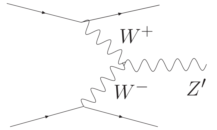
(b)

Figure 3: Representative Feynman diagrams for the $Z^{\prime}$ production channels.

To further quantify the search sensitivity to the ${Z^{\prime}}$, we will thus concentrate on the DY process shown in Fig. 3(a). We include the coherent sum of the $A_{1}$, $\tilde{Z}_{1}$ and $\tilde{Z}_{X1}$ contributions to a particular final state in the following. Throughout this section, we set $g_{R}=g_{L}\approx g$, the SM $SU(2)_{L}$ coupling. We include b-quarks in the initial state along with the light quarks. We use the CTEQ6.1M parton distribution functions [31] for all our numerical calculations. We have obtained the results in this section by incorporating our model into CalcHEP [32] and performed some checks by adding our model into Madgraph [33].

Figure 4: Total cross section for ${Z^{\prime}}$ production versus its mass, (a) with the coupling constant squared ($\lambda^{2}$) factored out as in Table 10 in Appendix B (for states in the KK eigenbasis, where $Z_{KK}$ includes $A_{1}$, $Z_{1}$ and ${Z_{X}}_{1}$, and the $q\bar{q}{Z_{X}}_{1}$ coupling is vanishingly small), and (b) with the absolute normalization for the couplings (for states in the mass eigenbasis).

5.1 $A_{1},\ \tilde{Z}_{X1}\rightarrow W^{+}W^{-}$

As seen from the discussion for the ${Z^{\prime}}$ decay in Sec. 4, $A_{1}$ and $\tilde{Z}_{X1}$ decay to $W^{+}W^{-}$ with substantial branching fraction of $30-40\%$, while for $\tilde{Z}_{1}$ it is down by more than one order of magnitude.

Figure 5: Distributions of the $WW$ final state (a) for $W^{+}W^{-}$ invariant mass variable (in GeV) of a 2 and 3 TeV ${Z^{\prime}}$ along with the SM $W^{+}W^{-}$ background, and (b) for rapidity of a $W$. These are after a ${p_{T}}_{W}>250~{}$GeV cut.

To gain a qualitative sense first, we consider the differential cross section for the signal with a mass of 2 and 3 TeV and the irreducible SM background of $W^{+}W^{-}$ pair production in Fig. 5, for (a) the invariant mass distributions $M_{WW}$, and for (b) the rapidity distribution $\eta_{W}$. These are after a ${p_{T}}_{W}>250$ GeV cut. The signal cross-section before any cuts is about 16 fb for a mass of 2 TeV, and 1.3 fb for 3 TeV mass. Based on the distributions, the signal can be enhanced relative to background by the application of suitable $M_{WW}$ and $\eta$ cuts. We see clearly the good signal observability, and we consider in the following how to realize these cuts using only the observable particles resulting from the decay of the two $W$’s. Additional sources of background will have to be contended with when one considers specific decay modes.

For the observable final states, we will not consider the fully hadronic mode for $WW$ decays due to the formidable QCD di-jet background. We will propose to focus on the purely-leptonic and semi-leptonic channels.

5.1.1 Purely leptonic channel:

We first consider the purely leptonic mode, ${Z^{\prime}}\to WW\to\ell\nu\ell\nu\ (\ell=e,\mu)$, which provide the clean channels from the observational point of view. The price to pay is the rather small branching ratio $BR(WW)\approx(2/9)^{2}=4/81$, in addition to the inability to reconstruct the total invariant mass due to the presence of two neutrinos carrying away missing momentum. We select the events with the basic acceptance cuts

$$p_{T\ell}>50\ {\rm GeV},\quad|\eta_{\ell}|<3,\quad\Delta R_{\ell\ell}>0.4,\quad\hbox to0.0pt{\hbox to7.95831pt{\hfil/\hfil}\hss}E_{T}>50\ {\rm GeV},$$ (11)

where $p_{T\ell},\ \eta_{\ell}$ are the transverse momentum and pseudo-rapidity of the charged leptons, $\Delta R_{\ell\ell}$ the separation of $\ell\ell$, and $\hbox to0.0pt{\hbox to7.95831pt{\hfil/\hfil}\hss}E_{T}$ the missing transverse energy due to the neutrinos. The leading irreducible backgrounds include $W^{+}W^{-}\to\ell^{+}\ell^{-}\hbox to0.0pt{\hbox to7.95831pt{\hfil/\hfil}\hss}E_{T}$ and $Z/\gamma^{*}\to\tau^{+}\tau^{-}\to\ell^{+}\ell^{-}\hbox to0.0pt{\hbox to7.95831pt{\hfil/\hfil}\hss}E_{T}$.

Figure 6: The differential cross-section from Drell-Yan production of 2 TeV ${Z^{\prime}}$ into the $WW$ final state followed by $W^{+}\rightarrow\ell^{+}\nu$ and $W^{-}\rightarrow\ell\bar{\nu}$ at the LHC (all horizontal axis masses in GeV) for (a) pseudo-rapidity distribution of the charged lepton, (b) invariant mass of the charged lepton pair, (c) the effective mass distribution, and (d) the cluster transverse mass distribution. These distributions are after the basic cuts.

Although we will not be able to fully reconstruct the resonant variable of the invariant mass $M_{WW}$, we form the “effective mass” and cluster transverse mass defined by

$$M_{eff}\equiv{p_{T}}_{\ell_{1}}+{p_{T}}_{\ell_{2}}+\hbox to0.0pt{\hbox to5.03125pt{\hfil/\hfil}\hss}p_{T},\quad{M_{T}}_{WW}\equiv 2\sqrt{{p^{2}_{T}}_{\ell\ell}+M_{\ell\ell}^{2}}.$$ (12)

In Fig. 6 we show the different characteristics of the backgrounds and the signal for a 2 and 3 TeV mass, for (a) the pseudo rapidity $\eta$ distribution, (b) the effective mass distribution, (c) invariant mass of the lepton pair, and (d) the cluster transverse mass distribution. The variable ${M_{T}}_{WW}$ ($M_{\ell\ell}$) should be broadly peaked at the resonance mass (half of it), the $M_{eff}$ gives the typical energy scale of the object produced. We are motivated to tighten up the kinematical cuts to further improve the signal observability. The cuts and results are shown in Table 2. We see that the backgrounds can be suppressed to the level of $S/B\sim 1$, but the signal rate is rather low. For a 2 TeV $Z^{\prime}$, it is conceivable to reach a 5$\sigma$ statistical sensitivity with an integrated luminosity of 100 ${\rm fb^{-1}}$, while for a 3 TeV $Z^{\prime}$ a higher luminosity would be needed to have a clear observation of the signal.

Table 2: $pp\rightarrow\ell^{+}\ell^{-}\hbox to0.0pt{\hbox to7.95831pt{\hfil/\hfil}\hss}E_{T}$ cross-section (in fb) for the signal with $M_{Z^{\prime}}=2$, 3 TeV and the $WW$ and $\tau\tau$ backgrounds, with cuts applied successively ($M_{eff}$ and $M_{T}$ are in TeV). The number of events and statistical significance are shown for 100 ${\rm fb}^{-1}$ ($M_{Z^{\prime}}=2$ TeV) and 1000 ${\rm fb}^{-1}$ (3 TeV), respectively.

$2$ TeV	Basic cuts	$|\eta_{\ell}|<2$	$M_{eff}>1$ TeV	$M_{T}>$1.75 TeV	# Evts	$S/B$	$S/\sqrt{B}$
Signal	$0.48$	$0.44$	0$.31$	$0.26$	$26$	$0.9$	$4.9$
$WW$	$82$	$52$	$0.4$	$0.26$	$26$
$\tau\tau$	$7.7$	$5.6$	$0.045$	$0.026$	$2.6$
$3$ TeV	Basic cuts	$|\eta_{\ell}|<2$	$1.5<M_{eff}<2.75$	$2.5<M_{T}<5$	# Evts	$S/B$	$S/\sqrt{B}$
Signal	$0.05$	$0.05$	$0.03$	$0.025$	$25$
$WW$	$82$	$52$	$0.08$	$0.04$	$40$	$0.6$	$3.8$
$\tau\tau$	$7.7$	$5.6$	$0.015$	$0.003$	$3$

5.1.2 Semi-leptonic channel:

To increase the statistics, we next consider the semi-leptonic mode when one $W$ decays as $W\rightarrow\ell\nu\ (\ell=e,\ \mu)$ while the other as $W\rightarrow jj^{\prime}$ ($j$ denotes a jet from a light quark). The branching ratio for this channel is $BR(WW)\approx 2/9\times 6/9\times 2=8/27$, and the factor of 2 is due to including both $\ell^{+}$ and $\ell^{-}$.

Figure 7: Distributions of the two jets resulting from $W\rightarrow jj$ from the Drell-Yan production of a 2 TeV ${Z^{\prime}}$ for (a) the separation $\Delta R$ and (b) the lab-frame opening angle.

Owing to the large mass of the ${Z^{\prime}}$, the two $W$’s are significantly boosted resulting in their decay products highly collimated in the lab-frame. To illustrate this we show in Fig. 7 the distribution of (a) the separation $\Delta R$ and (b) the lab-frame opening angle of the decay products of two fermions of the $W$ for $M_{Z^{\prime}}=2$ TeV. It can be seen from the figures that the separation is strongly peaked around 0.16, consistent with $2M_{W}/p_{T}$ for the opening angle. This kinematical feature has significant impact on the searches. The presently typical jet reconstruction cone size of $\Delta R=0.4$ will cause these two jets from the $W$ decay to be reconstructed likely as a single jet (albeit a fat jet), This means that we would pick up the SM single jet as a background for each $W$ decaying hadronically. For the leptonically decaying $W$, the charged lepton and the missing neutrino will be approximately collinear as well, rendering the accurate determination of the missing transverse energy difficult, although making the kinematics simpler.

As explained above, the two jets may not be resolvable due to collimation, and merged as a single jet, and thus the process $W(\rightarrow\ell\nu)+1$ QCD jet turns out to be the leading background, aside from the semileptonic decay from $WW$ production. We adopt the event selection criteria with the basic cuts

$$p_{T\ell}>50\ {\rm GeV},\quad|\eta_{\ell}|<1,\quad\Delta R_{\ell}>0.4,\quad\hbox to0.0pt{\hbox to7.95831pt{\hfil/\hfil}\hss}E_{T}>50\ {\rm GeV},$$ (13)

$$E_{Tj}>100\ {\rm GeV},\quad|\eta_{j}|<1,\quad\Delta R_{j}>0.4.$$ (14)

In order to capture the feature of the production of a very massive object, and to reconstruct the ${Z^{\prime}}$ mass, we once again consider the effective mass and the transverse mass defined as

$$M_{eff}\equiv{p_{T}}_{jj}+p_{T\ell}+\hbox to0.0pt{\hbox to5.03125pt{\hfil/\hfil}\hss}p_{T},\quad{M_{T}}_{WW}=2\sqrt{E_{Tjj}^{2}+M^{2}_{W}},$$ (15)

where $E_{Tjj}$ is the transverse energy for the jet pair which presumably reconstructs to the hadronic $W$. Alternatively, one can design a more sophisticated variable in the hope to reconstruct the invariant mass for the semi-leptonic system. This makes use of the fact that the missing neutrino is collimated with the charged lepton and we thus can expect to approximate the unknown longitudinal component of the $\nu$ momentum by

$$p_{L\nu}={\hbox to0.0pt{\hbox to7.95831pt{\hfil/\hfil}\hss}E_{T}\over p_{T\ell}}\ p_{L\ell}.$$ (16)

The momentum of the leptonic $W$ is thus reconstructed and we can evaluate the invariant mass of the semi-leptonic system by $\bar{M}_{WW}^{2}=(p_{\ell\nu}+p_{jj})^{2}$. In Fig. 8(a), we show the distributions for the two variables $M_{TWW}$ (solid curve) and $\bar{M}_{WW}$ (dashed curve) along with the continuum background. These variables reflect the resonant feature rather well. We find the following cuts effective in reducing the QCD background for two representative values of $M_{Z^{\prime}}$

$$M_{eff}>1000\ {\rm GeV},\quad 1800<M_{TWW}<2200\ {\rm GeV}\ {\rm for\ 2~{}TeV,}$$ (17)

$$M_{eff}>1250\ {\rm GeV},\quad 2800<M_{TWW}<3200\ {\rm GeV}\ {\rm for\ 3~{}TeV.}$$ (18)

Another approach could be to constrain $(p_{\ell}+p_{\nu})^{2}=M_{W}^{2}$ which allows us to infer the z-component of $p_{\nu}$ also, up to a quadratic ambiguity. Although the collimation of the $\ell\nu$ makes the mass determination inaccurate, it can be treated in a manner that maximizes signal over background. We do not pursue this method here.

Figure 8: Distributions for the signal and background (a) the reconstructed invariant mass $\bar{M}_{WW}$ (after $p_{T}$ and $\eta$ cuts), and (b) jet-mass distribution for a cone-size of 0.4 with and without $E$, $\eta$ and $\phi$ smearing.

In order to improve the rejection of QCD background, we may be able to exploit more differences between the signal and the QCD background (W+1jet). One such quantity that may have discriminating power is the jet-mass, which is the combined invariant mass of the vector sum of 4-momenta of all hadrons making up the jet. The jet-mass resolution is limited by our ability to reconstruct the angular separation of the constituents of the jet. For $M_{Z^{\prime}}$ in the few TeV range, due to collimation, forming the jet-mass becomes more challenging, since the cell size of the (ATLAS) hadronic calorimeter is of the order $\Delta\eta\times\Delta\phi\sim 0.1\times 0.1$. Although the two jets from $W\rightarrow jj$ are severely overlapping in the hadronic calorimeter, it may be possible to combine [34] it with the electromagnetic calorimeter and the tracker in order to obtain a reasonable discriminating power using the jet-mass. Since the EM calorimeter has better granularity, the two jets from the signal $W$ events are expected to have two separated EM cores, and the finer segmentation of the EM calorimeter helps in improving the jet-mass resolution [35]. For the signal, we expect the jet mass to peak at $M_{W}$, and, although a QCD jet will develop a mass due to the color radiation or showering, the jet-mass is limited when the jet size is fixed by $\Delta R$ and only single jet events are retained. We can thus use a jet-mass cut to suppress the QCD background. To obtain a rough estimate of how much background can be rejected, we have performed a study with the leading-order $W+1$ jet matrix element followed by showering in Pythia 6.4 [36]. In Fig. 8(b), we show the resulting jet-mass distributions for the signal and background where we have smeared the energy by $80$ %/$\sqrt{E}$ and the $\eta$ and $\phi$ by $0.05$ to account for possible experimental uncertainties. We find that for a jet-mass cut

$$75<M_{jet}<125\ {\rm GeV},$$ (19)

we obtain an acceptance fraction of $0.78$ for the signal, while it is $0.3$ for the background. It is important to emphasize that this level of study gives us a rough estimate, and a more realistic determination would require a study beyond leading order and including a detector simulation. A study along these lines albeit in a different context and cuts has been performed in Refs. [37].

Table 3: $pp\rightarrow\ell^{\pm}\hbox to0.0pt{\hbox to7.95831pt{\hfil/\hfil}\hss}E_{T}+1$ jet cross-section (in fb) for $M_{Z^{\prime}}=$2 and 3 TeV, and background, with cuts applied successively. The number of events is shown for ${\cal L}=100~{}{\rm fb}^{-1}$ for 2 TeV, and $1000~{}{\rm fb}^{-1}$ for 3 TeV.

$M_{Z^{\prime}}=2$ TeV	$p_{T}$	$\eta_{\ell,j}$	$M_{eff}$	$M_{T_{WW}}$	$M_{jet}$	# Evts	$S/B$	$S/\sqrt{B}$
Signal	$4.5$	$2.40$	$2.37$	$1.6$	$1.25$	$125$	$0.39$	$6.9$
W+1j	$1.5\times 10^{5}$	$3.1\times 10^{4}$	$223.6$	$10.5$	$3.15$	$315$
WW	$1.2\times 10^{3}$	$226$	$2.9$	$0.13$	$0.1$	$10$
$M_{Z^{\prime}}=3$ TeV
Signal	$0.37$	$0.24$	$0.24$	$0.12$	-	$120$	$0.17$	$4.6$
W+1j	$1.5\times 10^{5}$	$3.1\times 10^{4}$	$88.5$	$0.68$	-	$680$
WW	$1.2\times 10^{3}$	$226$	$1.3$	$0.01$	-	$10$

In Table 3 we show the cross-section (in fb) for the $pp\rightarrow\ell^{\pm}\hbox to0.0pt{\hbox to7.95831pt{\hfil/\hfil}\hss}E_{T}+1$ jet process for $M_{Z^{\prime}}=2$ and 3 TeV and the SM backgrounds of QCD and $W^{+}W^{-}$. The cuts as discussed in the text are applied successively and the improvement in $S/B$ is evident. For $M_{Z^{\prime}}=3$ TeV the increased collimation of the $W$ decay products makes it more challenging to use the jet-mass cut, and therefore we have not applied the jet-mass cut in this case. We find that the ${M_{T}}_{WW}$ cut results in a slightly better efficiency compared with the ${\bar{M}}_{WW}$ cut, and we therefore do not show the latter cut in the table. We thus infer for $M_{Z^{\prime}}=2$ TeV that a signal of about $7\sigma$ significance may be reached with an integrated luminosity of $100~{}\rm fb^{-1}$, with a $S/B=40\%$. A heavier $Z^{\prime}$ would need significantly more luminosity to see a clear signal. For instance, 1000 $\rm fb^{-1}$ may be needed to reach about a 5$\sigma$ sensitivity for $M_{Z^{\prime}}=3$ TeV.

5.2 $\tilde{Z}_{1}\rightarrow Zh$

Figure 9: The differential cross-section as a function of (a) the $Z\,h$ invariant mass, and (b) the ${p_{T}}_{Z}$, from Drell-Yan production of ${Z^{\prime}}$ (with mass 2 TeV and 3 TeV) at the LHC including the SM background. This is after the cuts ${p_{T}}_{Z,h}>200$GeV, and $-3<\eta_{Z,h}<3$.

As discussed in the last section, the $W^{+}W^{-}$ mode from $A_{1},\ \tilde{Z}_{X_{1}}$ decays will lead to significant signals; while their decay to $Zh$ will be small. On the other hand, the decay channel $\tilde{Z}_{1}\to Zh$ is overall dominant as seen from Fig. 2. We impose the basic acceptance cuts for the event selection

$${p_{T}}_{Z},\ {p_{T}}_{h}>200~{}{\rm GeV}\ \ ;\ \ -3<\eta_{Z},\ \eta_{h}<3\ .$$ (20)

After the basic cuts, the cross-section for $M_{Z^{\prime}}=2$ TeV into this final state is 16.7 fb for 2 TeV mass, and 1.8 fb for 3 TeV mass. Figure 9 shows the differential cross-section as a function of the $Zh$ invariant mass, and ${p_{T}}_{Z}$, along with the SM background arising from the $Zh$ production. Although the SM irreducible background from $Zh$ production is small, when a particular decay mode is considered we will pick up additional sources of background. Again due to the large boost of fast moving $Z$ and $h$, the decay products are collimated, making signal reconstruction more challenging. We will discuss these issues in greater detail in the following when we consider particular decay modes.

For our purposes of illustration here, most important features can be highlighted by considering two cases: $m_{h}=120~{}$GeV and $m_{h}=150~{}$GeV..

5.2.1 $m_{h}=120~{}$GeV

The $h$ decay modes in this mass range (with branching fractions in parenthesis) are: $b\bar{b}$ (0.7), $\tau^{+}\tau^{-}$ (0.07), $WW^{*}$ ($0.15$) and $ZZ^{*}$ (0.02). The leading Higgs decay is $h\to b\bar{b}$, we thus consider the leptonic modes of the $Z$ decay as

1. $h\rightarrow b\bar{b}$, $Z\rightarrow\ell^{+}\ell^{-}$: BR $\approx 0.7\times 2/30=4.6\%$. If the two $b$-jets get merged, we demand to tag only one $b$ to be conservative. The background with one tagged $b$ thus is $Z+1~{}b\to\ell^{+}\ell^{-}+1$ tagged $b$.

2. $h\rightarrow b\bar{b}$, $Z\rightarrow\nu\bar{\nu}$: BR $\approx 0.7\times 0.21=15\%$. Here we can demand a large missing $E_{T}$ (of the order $M_{Z^{\prime}}/2$). The background is mainly from $Z+1~{}b\to\hbox to0.0pt{\hbox to7.95831pt{\hfil/\hfil}\hss}E_{T}+1$ tagged $b$.

Obviously, the decay $Z\to\ell^{+}\ell^{-}$ yields a clean mode and we thus concentrate on the channel $pp\rightarrow b\bar{b}\ \ell^{+}\ell^{-}$. We start with the basic cuts as in Eq. (20), and we show the distributions after the cuts in Fig. 10. It should be noted that the signal distributions and cross-sections are obtained by multiplying the corresponding $Zh$ quantities by BR($h\rightarrow b\bar{b}$) and BR($Z\rightarrow\ell^{+}\ell^{-}$).

Figure 10: Signal and background distributions in $pp\rightarrow b\bar{b}\ell^{+}\ell^{-}$ for (a) $b\bar{b}\ell\ell$ invariant mass, (b) ${p_{T}}_{Z}$, (c) $\eta_{Z}$, and (d) $\cos{\theta_{Zb}}$. These are after the basic cuts.

For the ${Z^{\prime}}\rightarrow hZ\rightarrow b\bar{b}~{}\ell\ell$ mode we show the significance in Table 4 as we tighten up the cuts successively as follows

$${p_{T}}_{\ell}>250\ {\rm GeV},\ {p_{T}}_{b\bar{b}}>0.5\ {\rm TeV},\ \eta_{\ell,b}<2,\ \cos\theta_{\ell b}<-0.5,\ 1850<M_{Zh}<2150\ {\rm GeV}\ \ {\rm for\ 2~{}TeV,}~{}~{}~{}$$

$${p_{T}}_{\ell}>500\ {\rm GeV},\ {p_{T}}_{b\bar{b}}>1\ {\rm TeV},\ \eta_{\ell,b}<2,\ \cos\theta_{\ell b}<-0.5,\ 2800<M_{Zh}<3200\ {\rm GeV}\ \ {\rm for\ 3~{}TeV}.$$

We use a b-tagging efficiency of $0.4$ with a rejection factor for light-jets (from $u,d,s,g$) $R_{u}=20$ [38]. It is noted that this efficiency/rejection is with b-tagging parameters optimized for low ${p_{T}}_{b}$, and the rejection is expected to improve with tagging techniques optimized for high ${p_{T}}_{b}$. We use a charm quark rejection factor $R_{c}=5$. We find a clear signal above the background. With an integrated luminosity of 200 $\rm fb^{-1}$ (1000 $\rm fb^{-1}$), we obtain $S/\sqrt{B}\approx 5.3$ (5.7) for $M_{Z^{\prime}}=2$ TeV ($3$ TeV). Improvements in the b-tagging light-jet rejection factor can improve the significance even further.

Table 4: $pp\rightarrow Zh\rightarrow b\bar{b}~{}\ell\ell$ cross-section (in fb) for the signal with $M_{Z^{\prime}}=2$ TeV, and $M_{Z^{\prime}}=3$ TeV, and the corresponding backgrounds, with cuts applied successively. The statistical significance is shown for 200 ${\rm fb}^{-1}$ (for 2 TeV) and for 1000 ${\rm fb}^{-1}$ (for 3 TeV).

$M_{Z^{\prime}}=2$ TeV	Basic	$p_{T},\eta$	$\cos{\theta_{Zh}}$	$M_{inv}$	b-tag	# Evts	$S/B$	$S/\sqrt{B}$
$Z^{\prime}\rightarrow hZ\rightarrow b\bar{b}\,\ell\ell$	$0.81$	$0.73$	$0.43$	$0.34$	$0.14$	$27$	$1.1$	$5.3$
SM $Z+b$	$157$	$1.6$	$0.9$	$0.04$	$0.016$	$3$
SM $Z+b\bar{b}$	$13.5$	$0.15$	$0.05$	$0.01$	$0.004$	$0.8$
SM $Z+q_{l}$	$2720$	$48$	$22.4$	$1.5$	$0.08$	$15$
SM $Z+g$	$505.4$	$11.2$	$5.8$	$0.5$	$0.025$	$5$
SM $Z+c$	$184$	$1.9$	$1.1$	$0.05$	$0.01$	$2$
$M_{Z^{\prime}}=3$ TeV
$Z^{\prime}\rightarrow hZ\rightarrow b\bar{b}\,\ell\ell$	$0.81$	$0.12$	$0.05$	$0.04$	$0.016$	$16$	$2$	$5.7$
SM $Z+b$	$157$	$0.002$	$0.001$	$3\times 10^{-4}$	$1.2\times 10^{-4}$	$0.12$
SM $Z+b\bar{b}$	$13.5$	$0.018$	$0.014$	$0.002$	$0.001$	$1$
SM $Z+q_{l}$	$2720$	$1.1$	$0.7$	$0.1$	$0.005$	$5$
SM $Z+g$	$505.4$	$0.3$	$0.2$	$0.03$	$0.0015$	$1.5$
SM $Z+c$	$183.5$	$0.03$	$0.02$	$0.002$	$4\times 10^{-4}$	$0.4$

5.2.2 $m_{h}=150~{}$GeV

The $h$ decay modes in this mass range (with B.R.’s in parenthesis) are: $b\bar{b}$ (0.2), $\tau^{+}\tau^{-}$ (0.001), $WW^{*}$ (0.7) and $ZZ^{*}$ (0.1), we will thus consider the leading mode of $WW^{*}$. After including the $Z$ decay BR’s we find the following modes to be significant:

1. $h\rightarrow WW\to$jets, $Z\rightarrow\ell^{+}\ell^{-}$: BR $\approx 0.7\times(2/3)^{2}\times 1/15=2.1\%$. The corresponding background is from $Z+2$ jets $\to$ 2 jets $+\ell^{+}\ell^{-}$.

2. $h\rightarrow WW\to$ jets, $Z\rightarrow\nu\bar{\nu}$: BR $\approx 0.7\times(2/3)^{2}\times 0.2=6.2\%$. The background is from $Z+2$ jet $\to$ 2 jets $+\hbox to0.0pt{\hbox to7.95831pt{\hfil/\hfil}\hss}E_{T}$.

3. $h\rightarrow WW\to\ell\nu\ jj$, $Z\rightarrow jj$: BR$\approx 0.7\times(2\times 2/9\times 2/3)\times 0.7=15\%$. The background is from $W+2$ jets $\to$ 2 jets $+\ell^{\pm}+\hbox to0.0pt{\hbox to7.95831pt{\hfil/\hfil}\hss}E_{T}$.

We consider the last channel that yields the largest branching fraction with good experimental signatures. The $\Delta R$ separation of the two jets from the $W$ is about 0.3 and those from the $Z$ about 0.16. In our analysis, to be conservative, we will not require that the two jets be resolved and treat them as a single jet (one from the $W$ and another from the $Z$). We will refer to the jet(s) from the hadronic decay of the $W$ as the “near-jet” (since it is near to the leptonic $W$) and the jet(s) from the $Z$ as the “far-jet”. We will denote them as $j_{N}$ and $j_{F}$ respectively. The jet merging issues discussed in Sec. 5.1.2 are applicable identically to $j_{F}$, and much less severe for $j_{N}$ (due to larger $\Delta R\approx 0.3$).

The irreducible SM background will be due to $ZWW$. However, owing to the above jet merging issues, we will additionally pick up $WZj$, $WWj$ and $Wjj$. The former two are smaller than the last because of the electroweak versus the strong coupling.

Since the final state has a neutrino carrying away (missing) momentum we will not be able to reconstruct the full invariant mass of the system. We therefore use the transverse-mass of the $\ell j_{N}j_{F}$ system to enhance the signal resonance. The transverse mass is defined by

$${M_{T}}_{Zh}=\sqrt{{p_{T}}_{Z}^{2}+M_{Z}^{2}}+\sqrt{{p_{T}}_{h}^{2}+M_{h}^{2}}.$$ (21)

In Fig. 11 we compare the $M_{T}$ and the true invariant mass ($M_{inv}$). We see that the $M_{T}$ distribution reflects the resonant structure rather well, although it is broader.

Figure 11: The transverse mass distribution for the signal compared with the true invariant mass.

We select $\ell$ + 2-jet events with the following basic cut:

$${p_{T}}_{j}>100\ {\rm GeV},\ {p_{T}}_{\ell}>50\ {\rm GeV},\ \hbox to0.0pt{\hbox to5.03125pt{\hfil/\hfil}\hss}p_{T}>50\ {\rm GeV},\ |\eta_{\ell,j}|<3.$$ (22)

We further apply various cuts to improve the significance, which is shown in Table 5. For $M_{Z^{\prime}}=2$ TeV we apply successively the cuts:

$${p_{T}}_{j_{N}}>400\ {\rm GeV},\quad{p_{T}}_{j_{F}}>800\ {\rm GeV},$$ (23)

$$0.8<\cos{\theta_{Wj_{N}}}<1,\quad-1<\cos{\theta_{j_{N}j_{F}}}<-0.5,$$ (24)

$$1750\ {\rm GeV}<{M_{T}}_{Wj_{N}j_{F}}<2150\ {\rm GeV},\ \ 100<{M_{T}}_{Wj_{N}}<175\ {\rm GeV}\ \ ({\rm near}\ m_{h}),$$ (25)

$$70\ {\rm GeV}<M_{j_{F}}<110\ {\rm GeV}\ \ ({\rm near}\ M_{Z}).$$ (26)

Similarly for $M_{Z^{\prime}}=3$ TeV,

$${p_{T}}_{j_{N}}>500\ {\rm GeV},\quad{p_{T}}_{j_{F}}>1000\ {\rm GeV},$$ (27)

$$0.8<\cos{\theta_{Wj_{N}}}<1,\quad-1<\cos{\theta_{j_{N}j_{F}}}<-0.5,$$ (28)

$$2800\ {\rm GeV}<{M_{T}}_{Wj_{N}j_{F}}<3100\ {\rm GeV},\ \ 100<{M_{T}}_{Wj_{N}}<175\ {\rm GeV}\ \ ({\rm near}\ m_{h}).$$ (29)

Due to increased collimation we do not apply the jet-mass cut on $j_{F}$. Although we do not pursue it here we can apply a jet-mass cut on $j_{N}$ to further improve the significance. For the 3 TeV case, we only show the SM $Wjj$ background in Table 5 but not the $WZj$ and $WWj$ since they are much smaller as in the earlier case. Once again, we obtain substantial statistical significance for the signals.

Table 5: $pp\rightarrow Zh\rightarrow(jj)~{}(jj)~{}\ell\hbox to0.0pt{\hbox to7.95831pt{\hfil/\hfil}\hss}E_{T}$ cross-section (in fb) for the signal with $M_{Z^{\prime}}=2$ TeV and 3 TeV and the corresponding backgrounds, with cuts applied successively. The number of events and statistical significance are shown for 100 ${\rm fb}^{-1}$ (for 2 TeV) and 300 ${\rm fb}^{-1}$ (for 3 TeV).

$M_{Z^{\prime}}=2$ TeV   $m_{h}=150$ GeV	Basic	$p_{T},\eta$	$\cos{\theta}$	$M_{T}$	$M_{jet}$	# Evts	$S/B$	$S/\sqrt{B}$
$Z^{\prime}\rightarrow hZ\rightarrow\ell\,\hbox to0.0pt{\hbox to7.95831pt{\hfil/\hfil}\hss}E_{T}\,(jj)\,\,(jj)$	$2.4$	$1.6$	$0.88$	$0.7$	$0.54$	$54$	$2.5$	$11.5$
SM $W\,j\,j$	$3\times 10^{4}$	$35.5$	$12.7$	$0.62$	$0.19$	$19$
SM $W\,Z\,j$	$184$	$0.45$	$0.15$	$0.02$	$0.02$	$2$
SM $W\,W\,j$	$712$	$0.54$	$0.2$	$0.02$	$0.01$	$1$
$M_{Z^{\prime}}=3$ TeV   $m_{h}=150$ GeV
$Z^{\prime}\rightarrow hZ\rightarrow\ell\,\hbox to0.0pt{\hbox to7.95831pt{\hfil/\hfil}\hss}E_{T}\,(jj)\,\,(jj)$	$0.26$	$0.2$	$0.14$	$0.06$	$-$	$18$	$1.2$	$4.7$
SM $W\,j\,j$	$3\times 10^{4}$		$4.1$	$0.05$	$-$	$15$

5.3 ${Z^{\prime}}\rightarrow\ell^{+}\ell^{-}$

The cleanest channel of all should be the di-lepton mode from the DY production. However, due to the highly suppressed coupling of $Z^{\prime}$ to the light fermions, this channel requires a large integrated luminosity for observation. The cross-section into the $\ell^{+}\ell^{-}$ final state (with $\ell=e,\mu$) for $M_{Z^{\prime}}=2~{}$ TeV is 0.12 fb without any cuts. We select events with the basic cuts

$${p_{T}}_{\ell}>50\ {\rm GeV},\quad|\eta_{\ell}|<3.$$ (30)

In Table 6 we show the improvement in S/B for $M_{Z^{\prime}}=2$ TeV as we apply the following cuts:

$${p_{T}}_{\ell}>500\ {\rm GeV},\quad 1900\ {\rm GeV}<M_{\ell\ell}<2100\ {\rm GeV}.$$ (31)

One would need much larger integrated luminosity to reach a significant signal. Although the event rate is rather low and high luminosity would be needed to reach a significant observation, it is noted that this clean channel is mainly statistically dominated and does not suffer from systematic effects present in some of the other channels.

Table 6: $pp\rightarrow\ell^{+}\ell^{-}$ cross-section (in fb) for $M_{Z^{\prime}}=2$ TeV signal and the corresponding backgrounds, with cuts applied successively. The number of events and statistical significance are shown for 1000 ${\rm fb}^{-1}$.

$M_{Z^{\prime}}=2$ TeV	Basic	$p_{T\ell}$	$M_{\ell\ell}$	# Evts	$S/B$	$S/\sqrt{B}$
Signal	$0.1$	$0.09$	$0.06$	$60$	$0.3$	$4.2$
SM $\ell\ell$	$3\times 10^{4}$	$5.4$	$0.2$	$200$
SM $WW$	$295$	$0.03$	$0.002$	$2$

5.4 ${Z^{\prime}}\rightarrow t\bar{t},\ b\bar{b}$

Because of the large coupling to the heavy fermions, the decay modes of $Z^{\prime}$ to $t\bar{t},\ b\bar{b}$ are substantial. We start with the basic cut

$${p_{T}}_{t}>100\ {\rm GeV},\quad|\eta_{t}|<3.$$ (32)

Figure 12: The differential cross-section of Drell-Yan production of 2 and 3 TeV signal and SM background, as a function of ${p_{T}}_{t}$ (left), and $M_{tt}$ (right), after basic cuts. The KK gluon contribution has not been included in these plots.

Fig. 12 shows the Drell-Yan cross-section of ${Z^{\prime}}$ with mass 2 and 3 TeV into the $t\bar{t}$ final state after basic cuts.

Table 7: $pp\rightarrow t\bar{t}$ cross-section (in fb) for $M_{Z^{\prime}}=2$ and $3$ TeV signal and the corresponding SM backgrounds, with cuts applied successively ($p_{T}$ and $M_{\ell\ell}$ are in GeV).

$M_{Z^{\prime}}=2$ TeV	Basic	$p_{T}>800$	$1900<M_{tt}<2100$
Signal	$17$	$7.2$	$5.6$
SM $t\bar{t}$	$1.9\times 10^{5}$	$31.1$	$19.1$
$M_{Z^{\prime}}=3$ TeV	Basic	$p_{T}>1250$	$2850<M_{tt}<310$
Signal	$1.7$	$0.56$	$0.45$
SM $t\bar{t}$	$1.9\times 10^{5}$	$4.1$	$1.1$

In Table 7 we show the cross-section as we tighten the cuts without including any top decay branching ratios. We see that the signal observability over the SM background is promising at this level.

The fully hadronic mode from $t\bar{t}$ decays to $b\bar{b}+4j$ has a branching fraction about BR$\approx 0.65^{2}=43\%$. In the hadronic mode, we expect for a 2 TeV ${Z^{\prime}}$ that the $jj$ opening angle of $jj$ from the $W$ is $2M_{W}/p_{T}\sim 0.32$ rad. The multiple-jet QCD background Will be difficult to overcome making this decay channel difficult to observe. The semi-leptonic mode for $\ell=e,\mu$ has with BR$=0.65\times 0.12\times 2\times 2=31\%$ and the event reconstruction has been discussed in Refs. [39], and the signal significance is found to be encouraging consistent with Table 7.

Now we turn to ${Z^{\prime}}\rightarrow b\bar{b}$. The ${Z^{\prime}}$ cross-section for $M_{Z^{\prime}}=2~{}$TeV into this final state is 8.4 fb without any cuts. With the cuts

$$|\eta_{b,\bar{b}}|<1,\quad 1900\ {\rm GeV}<M_{bb}<2100\ {\rm GeV}\ ,$$ (33)

the cross-section is $\sigma_{S}=0.7$ fb, while the SM background with the same cuts is $\sigma_{B}=14.9$ fb. The significance is thus marginal for this channel.

Figure 13: The KK gluon and ${Z^{\prime}}$ line-shapes at the peak. The dotted line is the BW shape due to the KK gluon. The dashed line is due to the 3 neutral modes. The solid line is the sum. The error-bars shown are statistical only for the indicated integrated luminosity.

However, as discussed in recent literature [2], the KK gluon ($G_{1}$) contributes dominantly to the $t\bar{t}$ mode with a cross-section of about $938$ fb without any cuts for the $M_{Z^{\prime}}=2$ TeV case, and is $108$ fb after the cuts similar to Eq. (33). This large production rate may prohibit the observation of the $Z^{\prime}$ in this channel. This is illustrated in Fig. 13, where we see that a $Z^{\prime}$ peak may be totally buried under the $G_{1}$ signal.

Note that, like in the case of the SM $Z$ boson, the ${Z^{\prime}}$ will induce a tree-level forward-backward asymmetry (or charge asymmetry) that can be observed via the the distribution of the $t\bar{t}$ and $b\bar{b}$ final states. The SM predicts a very small asymmetry which is dominantly due to next to leading order QCD processes (NLO)[40] (in $q\bar{q}$ annihilation) which are further diluted at the LHC due to fact that the production is dominated by $gg$ fusion. Interestingly enough, since the KK gluon is dominantly produced via $q\bar{q}$ annihilation then the asymmetry due to the NLO processes will be enhanced and expected to be of $\cal O$ (10%). Furthermore, near the peak of ${Z^{\prime}}$ the ratio between the KK gluon background and the signal is roughly about ten (depends on how degenerate they are). The nondegeneracy between the KK gluon and ${Z^{\prime}}$ masses can be generated for example from loop corrections to the brane kinetic terms [41], and we illustrate its effect in the lower panel of Fig. 13. The ${Z^{\prime}}$ would yield an additional source of forward backward asymmetry roughly at the same size (after taking into account the ratio of cross sections). If measured, this pattern, in the asymmetries associated with the location of the KK gluon and the location of the ${Z^{\prime}}$ resonance would yield an intriguing hints that the signal indeed originated from the above set-up. Since the new boson would generically decay dominantly either to RH or LH tops we expect that the sign of the resulting left-right polarization asymmetry would be the same as the one induced by the KK gluon (see the first Ref. in [2]).

6 Conclusions

The Randall-Sundrum I (RS1) framework of a warped extra dimension provides a novel and very interesting resolution to the Planck-weak and flavor hierarchy problem of the SM. As we enter the LHC era, however, it is of crucial importance to know the prospects for experimentally verifying this framework. This amounts to observing the Kaluza-Klein (KK) excitations of bulk fields in RS1 and measuring their couplings.

Considerations related to flavor and electroweak (EW) physics, as well as the requirement of UV insensitivity, suggest that the SM fields may propagate in the bulk, with the light fermions being localized near the UV brane (Planck brane) and heavier fermions closer to the IR brane (TeV brane). The resulting setup leads to two serious challenges for the LHC phenomenology: (i) KK couplings to light fermions, and in particular to proton’s constituents, are suppressed since the KK states are localized near the TeV brane. (ii) The dominant decay channels of the new states is to TeV-brane localized fields, namely longitudinal gauge bosons, the Higgs and third generation quarks. These features make most of the new states rather elusive.

Nonetheless, it was shown in Ref. [2] that a KK gluon with a mass up to $\cal O$(4 TeV) is within the reach of the LHC. However, observing a single KK state would not suffice to verify the above class of models. The aforementioned challenging features were shown to make the discovery of a KK graviton questionable, unless it is unexpectedly light [3].

In this work, we considered the corresponding neutral KK states of the EW sector. We focused on a class of models with custodial symmetry for $Z\to b\bar{b}$ (and the $\rho$ parameter). In these models in addition to the SM fields, there are three neutral KK modes present, denoted collectively as $Z^{\prime}$, with masses of order of a few TeV, in compliance with precision tests.

In accordance with the above discussion, we find that discovering these states is a non-trivial task. The leading production channel is the Drell-Yan process. We investigated various decay modes and analysis strategies. We showed that, unlike the often studied $Z^{\prime}$ cases, the LHC $Z^{\prime}$ mass reach for the above RS1 models is more limited, where KK states of mass $\sim 2\;(3)$ TeV can be discovered with a $\sim 100$ fb^-1 ($\sim 1$ ab^-1) of integrated luminosity. Since the electroweak and flavor precision tests favor KK mass $\gtrsim 3$ TeV in the simplest existing models, our results clearly motivate luminosity upgrade for the LHC. The best discovery mode is via a $Zh$ (a $Z$ and a Higgs) final state which works both for a light and heavy Higgs. The assumption here is that the decays of the Higgs are dominated by SM final states and the corresponding branching fractions are approximately like in the SM.

However, only one of the three neutral eigenstates dominantly decays into the $Zh$ final state. We demonstrated that the two other modes can be discovered via longitudinal $WW$ final state, although it will require a higher luminosity. The $WW$ semi-leptonic mode (in general modes in which the $W$ and $Z$ decay hadronically) will benefit from unconventional jet-mass reconstruction techniques that may be devised in the future. It is worth noting, in addition, that with enough statistics one can look at the $W/Z$ polarization, associated with the signal in the differential cross section, and observe that they are dominantly longitudinally polarized as predicted by our framework.

The three neutral states have a sizable branching ratio into top pairs. However, they tend to be degenerate in mass with the KK gluon so that the signal is completely swamped by KK gluon decay into tops. Precision measurements of the top final state, such as forward backward asymmetry can, nevertheless, allow for indirectly observing the presence of the $Z^{\prime}$.

Finally, we emphasize that, via the AdS/CFT duality [5], the RS framework can be viewed as a tool to study $4D$ strong dynamics. In fact, the idea of a composite pseudo-Goldstone boson (PGB) Higgs, in $4D$, has been studied in the RS framework (called “holographic” PGB Higgs) [7, 8]. It is therefore likely that our results apply (in general) to $4D$ TeV-scale strong dynamics responsible for EWSB. In particular, our analysis with regard to the RS1 LHC signals suggests that little hierarchy models with UV completion via strong dynamics (i.e., little Higgs and some flat extra dimensional models) would be characterized by LHC signals which are quite different from those usually emphasized in the literature. The reason is that the couplings between the extended electroweak sector and the light (heavy) SM particles may be actually highly suppressed (enhanced), unlike what is typically assumed in other LHC studies. Generically, the new particles will be broader, with small production rates and non-leptonic decay channels. As such, these models may face similar challenges regarding the detection of new states.

Appendix A Model details and Heavy Electroweak Gauge Bosons

This section describes the couplings of $1$ heavy $W$ or $Z$ state to $2$ SM states in a model with the SM gauge fields propagating in the bulk of a warped extra dimension and the Higgs being localized close to the TeV brane. In subsection A.1, we begin with couplings of heavy $W$ or $Z$ to (i) $2$ SM $W$ or $Z$ and (ii) Higgs and SM $W$ or $Z$, considering first the simplified case of a single $SU(2)$ and giving a detailed derivation of the couplings in unitary gauge. Since these unitary gauge couplings have not been explicitly derived in the literature before to our knowledge, we feel that such a pedagogical treatment will be useful. If the reader wishes, she/he can skip the derivation and go directly to the couplings in Eq. (41) for the simplified case. We give a check against equivalence theorem in subsection A.1.3, followed by an outline only of the derivation of the same couplings for the realistic case in subsection A.2. Finally, in subsection A.3, we discuss the couplings of heavy $W$ or $Z$ to fermions with the charge assignments of reference [15] and in subsection A.4, we consider the charge assignments of reference [23] with the custodial symmetry for $Zb\bar{b}$. Various expressions directly relevant to our numerical study are summarized in App. B.

A.1 Simplified case of single $SU(2)$

A.1.1 Couplings to two SM $W$ or $Z$ in unitary gauge

The basic idea is that there are no couplings of $2$ gauge zero-modes to $1$ gauge KK mode at tree-level due to flatness of zero-mode profile and orthogonality of profiles. However, Higgs vev mixes zero and KK modes of $W$ so that mass eigenstates – “heavy” $W$ and SM $W$ – are admixtures of the two, with former being mostly KK $W$ and the latter being mostly zero-mode $W$. So, we can start with a coupling of $3$ $W$ zero-modes or a coupling of $2$ $W$ KK modes and $1$ $W$ zero-mode and use the above mixing to obtain a coupling of $1$ heavy $W$ to $2$ SM $W$. There are also couplings with $3$ KK modes which requires mixing twice to obtain coupling of $1$ heavy $W$ to $2$ SM $W$ and hence will be a higher order effect.

The mass terms (restricting to only zero and 1st KK modes) are

$$\frac{1}{4}g^{(0)\;2}v^{2}\Big{[}W^{+\;(0)}W^{-\;(0)}+\sqrt{k\pi r_{c}}W^{+\;(0)}W^{-\;(1)}\;(+\;h.c.)+k\pi r_{c}W^{+\;(1)}W^{-\;(1)}+$$

$$\frac{1}{2}W^{3\;(0)}W^{3\;(0)}+\sqrt{k\pi r_{c}}W^{3\;(0)}W^{3\;(1)}\;+\frac{1}{2}k\pi r_{c}W^{3\;(1)}W^{3\;(1)}\Big{]}+$$

$$m^{2}_{W^{(1)}}\Big{[}W^{+\;(1)}W^{-\;(1)}+\frac{1}{2}W^{3\;(1)}W^{3\;(1)}\Big{]}$$ (34)

where $g^{(0)}=g_{5D}/\sqrt{\pi r_{c}}$ is the zero-mode (or $4D$) gauge coupling. The factor of $\xi\equiv\sqrt{k\pi r_{c}}$ comes from the enhanced coupling of the Higgs that is peaked near the TeV brane to gauge KK modes, in turn, due to enhanced wavefunction of KK modes compared to zero-mode at the TeV brane. Also, the KK mass is

$$m_{W^{(1)}}\equiv m_{KK} \approx 2.45\;k\;e^{-k\pi r_{c}}$$ (35)

where (as usual) $k\pi r_{c}\sim\log\left(M_{Pl}/\hbox{TeV}\right)\sim 34$ and $k\sim M_{Pl}$ so that $m_{W^{(1)}}\sim$ (a few) TeV. We define

$$\xi\equiv\sqrt{k\pi r_{c}}\ ,$$ (36)

and we take $\xi=\sqrt{34}=5.83$ for our numerical study.

The mass eigenstates, denoted by $W$ (“SM”) and $W^{\prime}$ (heavy $W$), are

$$W^{(1)} \approx \cos\theta W^{\prime}+\sin\theta W$$

$$W^{(0)} \approx \cos\theta W-\sin\theta W^{\prime}$$ (37)

where

$$\tan 2\theta = \frac{\frac{1}{2}g^{(0)\;2}v^{2}\sqrt{k\pi r_{c}}}{m_{W^{(1)}}^{2}+\frac{1}{4}g^{(0)\;2}v^{2}\left(k\pi r_{c}-1\right)}$$ (38)

valid for both charged and neutral $W$. Clearly, the mass and couplings of SM $W$ are shifted relative to those of the zero-mode due to the above mixing with the KK mode, but this effect can be neglected for our purposes since it will be higher order in $v/m_{KK}$. So, we set $1/2\;g^{(0)}v\approx m_{W}$ and $g^{(0)}\approx g$, i.e., the SM $SU(2)_{L}$ gauge coupling, also denoted by $g_{L}$. Assuming $m_{W}^{2}\;k\pi r_{c}\ll m_{KK}^{2}$ (which holds for $m_{KK}\stackrel{{\scriptstyle>}}{{\sim}}$ a few TeV), we get

$$\sin\theta \approx \frac{m_{W}^{2}\sqrt{k\pi r_{c}}}{m_{KK}^{2}}$$ (39)

The Feynman rules in KK basis are (1) $3$ zero-mode couplings:

$$W^{+\;(0)}_{\nu}\left(k_{2}\right)W^{-\;(0)}_{\lambda}\left(k_{3}\right)W^{3\;(0)}_{\mu}\left(k_{1}\right) : -ig\Big{[}\left(k_{1}-k_{2}\right)_{\lambda}g_{\mu\nu}+\left(k_{2}-k_{3}\right)_{\mu}g_{\nu\lambda}+\left(k_{3}-k_{1}\right)_{\nu}g_{\lambda\mu}\Big{]}$$ (40)

and (2) KK $W^{3}$, KK $W^{-}$ and $W^{+}$ zero-mode and (3) KK $W^{3}$, KK $W^{+}$ and $W^{-}$ zero-mode coupling which are identical to that in Eq.(40). As mentioned above, the $3$ KK $W$ coupling will give a higher order effect.

We now go from the KK basis to the mass eigenstate basis using Eq. (37). Schematically, we use the above mixing to “convert” $W^{3}$ zero-mode to heavy $W^{3}$ in coupling (1) in Eq. (40) (which gives a factor of $\sin\theta$) and convert KK $W^{\pm}$ to SM $W^{\pm}$ in couplings (2) and (3) (which gives a factor of $-\sin\theta$). Thus, we obtain a coupling of $1$ heavy $W_{3}$ to SM $W^{-}$ and SM $W^{+}$ (setting $\cos\theta\approx 1$):

$$W^{+}_{\nu}\left(k_{2}\right)W^{-}_{\lambda}\left(k_{3}\right)W^{3\;\prime}_{\mu}\left(k_{1}\right) : -ig\sin\theta\Big{[}\left(k_{1}-k_{2}\right)_{\lambda}g_{\mu\nu}+\left(k_{2}-k_{3}\right)_{\mu}g_{\nu\lambda}+\left(k_{3}-k_{1}\right)_{\nu}g_{\lambda\mu}\Big{]}$$ (41)

with $\sin\theta$ given in Eq. (39).

Similarly couplings of heavy $W^{+}$ to SM $W_{3}$ and SM $W^{-}$ can be obtained.

A.1.2 Couplings to Higgs and SM $W$ or $Z$

¿From Eq. (34), i.e., replacing single $v$ by physical Higgs ($h$), and going from KK to mass basis, we get (setting $g^{(0)}\approx g$, $g^{(0)}v/2\approx m_{W}$ and $\cos\theta\approx 1$)

$${\cal L}_{Higgs} \approx m_{W}g\sqrt{k\pi r_{c}}h\Big{[}W^{3\;\prime}W^{3}+W^{+\;\prime}W^{-}(+h.c.)\Big{]}$$ (42)

A.1.3 Check against Equivalence Theorem

From Eq. (34), we can see that the couplings of complex Higgs doublet ($H$) to a single gauge KK mode only are given by $\sim\partial_{\mu}H^{\dagger}HW^{(1)}g\sqrt{k\pi r_{c}}$ – to be explicit, replace $g^{(0)}W^{(0)}$ by $\partial_{\mu}$ and $v/\sqrt{2}$ by $H$ in 2nd term of Eq. (34). By equivalence theorem, longitudinal $W$ and $Z$ are (approximately) the unphysical Higgs and hence the coupling of heavy $W$ to (i) 2 longitudinal SM $W$’s and also to (ii) physical Higgs and longitudinal SM $W$ is expected to be of the above size, i.e., $W_{long.}W_{long}W^{\prime}$ and $W_{long.}hW^{\prime}$ couplings $\sim g\sqrt{k\pi r_{c}}$ (up to the factor of derivative/momentum). Using the longitudinal polarization vector ($\sim E/m_{W}$) with $E\sim m_{KK}$ (which is valid for production/decay of heavy $W$), we do indeed get same result in unitary gauge from Eq. (41) and similarly from Eq. (42).

A.2 Realistic case

We have the gauge group $SU(2)_{L}\times SU(2)_{R}\times U(1)_{X}$ in the bulk with the SM Higgs doublet being promoted to a bi-doublet of $SU(2)_{L}\times SU(2)_{R}$, i.e., $\left(H,i\sigma_{2}H^{\ast}\right)$ transform as a doublet of $SU(2)_{R}$, where $H$ and $i\sigma_{2}H^{\ast}$ are each doublets of $SU(2)_{L}$ as usual and does not carry any $U(1)_{X}$ charge. The charged boson matrix is

$$\left(\begin{array}[]{ccc}W_{L}^{+\;(0)}&W_{L_{1}}^{+}&W_{R_{1}}^{+}\end{array}\right){\cal M}_{charged}^{2}\left(\begin{array}[]{c}W_{L}^{-\;(0)}\\ W_{L_{1}}^{-}\\ W_{R_{1}}^{-}\end{array}\right)$$ (47)

with

$${\cal M}_{charged}^{2} = \left(\begin{array}[]{ccc}m_{W}^{2}&m_{W}^{2}\sqrt{k\pi r_{c}}&-m_{W}^{2}\sqrt{k\pi r_{c}}\frac{g_{R}}{g}\\ m_{W}^{2}\sqrt{k\pi r_{c}}&m_{KK}^{2}+m_{W}^{2}k\pi r_{c}&-m_{W}^{2}k\pi r_{c}\frac{g_{R}}{g}\\ -m_{W}^{2}\sqrt{k\pi r_{c}}\frac{g_{R}}{g_{L}}&-m_{W}^{2}k\pi r_{c}\frac{g_{R}}{g}&0.963\;m_{KK}^{2}+m_{W}^{2}k\pi r_{c}\left(\frac{g_{R}}{g}\right)^{2}\end{array}\right)$$ (51)

where we have restricted to only the first KK modes, denoted by $W^{\pm}_{L_{1},\;R_{1}}$. Note that there is no zero-mode for $W_{R}^{+}$ due to choice of Dirichlet boundary condition (BC) on Planck brane so that $g_{R}$ is the “would-be” zero-mode (or $4D$) $SU(2)_{R}$ gauge coupling. Due to the different BC on Planck brane relative to $W^{+}_{L}$, the KK mass for $W^{+}_{R_{1}}$ is also slightly smaller:

$$M_{W^{+}_{R_{1}}} \approx 0.981\;m_{KK}$$ (52)

The mass eigenstates – $W$ (SM) and $\tilde{W}_{L_{1}}$, $\tilde{W}_{R_{1}}$ (two heavy $W$’s) – are mixtures of these $3$ modes. Note that (EW preserving) KK masses for $W^{+}_{R_{1}}$ and $W_{L_{1}}^{+}$ are quite degenerate such that the EWSB mixing (mass)² term is larger than KK (mass)² splitting for $m_{KK}\stackrel{{\scriptstyle<}}{{\sim}}3.5$ TeV. Hence, for the interesting range of KK masses, we expect large mixing between $W_{R_{1}}^{+}$ and $W_{L_{1}}^{+}$, i.e., $\tilde{W}_{L_{1}}$ and $\tilde{W}_{R_{1}}$ will be roughly $50-50$ admixtures of $W_{R_{1}}^{+}$ and $W_{L_{1}}^{+}$, of course with a small component of $W_{L}^{+(0)}$.

In the neutral gauge boson sector, it is convenient to define the KK $Z$ (denoted by $Z_{\mu}^{(1,\;2...)}$) and KK photon (denoted by $A_{\mu}^{(1,\;2,...)}$) to be linear combinations of KK $W^{3}_{L}$, i.e., $W^{3\;(1,\;2,...)}_{L}$, and KK hypercharge, i.e., $B^{(1,\;2,...)}$, with mixing identical to that for zero-modes, i.e.,

$$A_{\mu}^{(n)} = \sin\theta_{W}W_{\mu\;L}^{3\;(n)}+\cos\theta_{W}B^{(n)}_{\mu}$$

$$Z_{\mu}^{(n)} = \cos\theta_{W}W_{\mu\;L}^{3\;(n)}-\sin\theta_{W}B^{(n)}_{\mu}$$ (53)

where $n=0,1...$ and with $\sin\theta_{W}$ being the ratio of $4D$ (or zero-mode) hypercharge and $Z$ gauge couplings or equivalently the $5D$ hypercharge and $5D$ $Z$ gauge couplings, where $g_{5D\;Z}\equiv\sqrt{g_{5D\;L}^{2}+g_{5D\;Y}^{2}}$. In turn, the hypercharge gauge boson KK modes are linear combinations of KK modes of $U(1)_{R}$ and $U(1)_{X}$ gauge boson (denoted by $X_{\mu}^{(1,\;2,...)}$), with the combination orthogonal to hypercharge gauge boson being denoted by $Z_{X}$, i.e.,

$$B_{\mu}^{(n)} = \sin\theta^{\prime}W_{\mu\;R}^{3\;(n)}+\cos\theta^{\prime}X_{\mu}^{(n)}$$

$$Z_{\mu\;X}^{(n)} = \cos\theta^{\prime}W_{\mu\;R}^{3\;(n)}-\sin\theta^{\prime}X_{\mu}^{(n)}$$ (54)

In analogy with $B-W^{3}_{L}$ mixing, we have $\sin\theta^{\prime}=g_{X}/g_{Z^{\prime}}$, where $g_{Z^{\prime}}=\sqrt{g_{R}^{2}+g_{X}^{2}}$ and $g_{X}$ are the “would-be” zero-mode ($4D$) couplings for $Z_{X}$ and $U(1)_{X}$, respectively. Note that since the hypercharge gauge coupling, $g^{\prime}=g_{R}\;g_{X}/\sqrt{g_{R}^{2}+g_{X}^{2}}$, there is only $1$ gauge coupling (say, either $g_{R}$ or $g_{Z^{\prime}}$) which is a free parameter. See reference [15] for more details.

The photon and $Z$ KK masses are given by

$$M_{A_{1},\;Z_{1}} = m_{KK}$$ (55)

since both have Neumann BC’s on both branes. Whereas $Z_{X}$ does not have a zero-mode due to (effectively) Dirichlet BC on Planck brane so that

$$M_{{Z_{X}}_{1}} \approx 0.981\;m_{KK}$$ (56)

Here, we have denoted the first KK excitation of the three neutral gauge bosons as $A_{1}$, $Z_{1}$ and ${Z_{X}}_{1}$.

The advantage of this definition of KK $Z$ and KK photon is that the photon (zero and KK) modes do not couple to Higgs at leading order and hence do not mix with each other or with $Z_{1}$ or ${Z_{X}}_{1}$ modes even after EWSB. Hence, the SM photon is the zero-mode photon, i.e., EM coupling is not modified with respect to that of the zero-mode (this is guaranteed by $4D$ gauge invariance), unlike for the case of $W$ and $Z$.

Similar to the case of charged gauge bosons, the neutral gauge boson mass matrix is

$$\left(\begin{array}[]{ccc}Z^{(0)}&Z_{1}&{Z_{X}}_{1}\end{array}\right)\frac{1}{2}{\cal M}_{neutral}^{2}\left(\begin{array}[]{c}Z^{(0)}\\ Z_{1}\\ {Z_{X}}_{1}\end{array}\right)$$ (61)

$${\cal M}_{neutral}^{2} = \left(\begin{array}[]{ccc}m_{Z}^{2}&m_{Z}^{2}\sqrt{k\pi r_{c}}&-m_{Z}^{2}\sqrt{k\pi r_{c}}\frac{g_{Z^{\prime}}}{g_{Z}}{c^{\prime}}^{2}\\ m_{Z}^{2}\sqrt{k\pi r_{c}}&m_{KK}^{2}+m_{Z}^{2}k\pi r_{c}&-m_{Z}^{2}\;k\pi r_{c}\frac{g_{Z^{\prime}}}{g_{Z}}{c^{\prime}}^{2}\\ -m_{Z}^{2}\sqrt{k\pi r_{c}}\frac{g_{Z^{\prime}}}{g_{Z}}{c^{\prime}}^{2}&-m_{Z}^{2}\;k\pi r_{c}\frac{g_{Z^{\prime}}}{g_{Z}}{c^{\prime}}^{2}&0.963\;m_{KK}^{2}+m_{Z}^{2}k\pi r_{c}\left(\frac{g_{Z^{\prime}}}{g_{Z}}{c^{\prime}}^{2}\right)^{2}\end{array}\right)$$ (65)

where ${c^{\prime}}\equiv\cos{\theta^{\prime}}$.

As before, we start with the gauge couplings in KK basis – of $3$ zero-modes or $1$ zero-mode and $2$ KK modes – and use zero-KK mode mixing (i.e., go to mass eigenstate basis) to obtain couplings of $1$ heavy $W$ (or $Z$) to $2$ SM $W$ or $Z$.

In addition to the trilinear gauge couplings from $SU(2)_{L}$ group, we also need to take into account those from $SU(2)_{R}$. Note that $W_{R}^{\pm}$ does not have zero-modes so that there are no $3$ zero-mode couplings from $SU(2)_{R}$. However, the $W_{R}^{+\;(1)}$-$W_{R}^{-\;(1)}$-$W_{R}^{3\;(0)}$ coupling does contribute to the coupling of heavy $W$ to SM $W$ and SM $Z$ via mixing of $W^{+(1)}_{R}$ with $W_{L}^{+(0)}$, i.e., SM $W$ has a (small) admixture of $W_{R}^{+\;(1)}$.

Coupling of KK photon to $WW$

We also obtain a coupling of KK photon to 2 SM $W$’s via trilinear $SU(2)_{L}$ coupling between $W_{L}^{3\;(1)}$, $W_{L}^{\pm(1)}$ and $W_{L}^{\mp(0)}$ followed by $W_{L}^{\pm(1)}$ mixing with $W_{L}^{\pm(0)}$ via Higgs vev – the point is that the KK photon has an admixture of $W_{L}^{3\;(1)}$. It is clear that we cannot obtain such a coupling of KK photon from trilinear $SU(2)_{R}$ coupling (at the same order in $v/m_{KK}$). We can also obtain this coupling from equivalence theorem, i.e., coupling of KK photon to (unphysical) charged Higgs.

A.3 Couplings of fermions to heavy $W/Z/\gamma$

Here we take $U(1)_{X}$ to be $U(1)_{B-L}$ as usual. Neglecting effects suppressed by SM Yukawa couplings, couplings of (zero-modes of) light quarks (including $b_{R}$ and excluding $(t,b)_{L}$ and $t_{R}$) to electroweak gauge KK modes in weak/KK basis are suppressed by $\sim\xi\equiv\sqrt{k\pi r_{c}}\sim 5$ compared to the SM couplings:

$${\cal L} \ni \frac{-1.13}{\xi}\left(\frac{g_{Z}}{2}Z_{1}\,{}_{\mu}\Big{[}\bar{u}\gamma^{\mu}\left(\frac{1}{2}-\frac{4}{3}\sin^{2}\theta_{W}-\frac{1}{2}\gamma_{5}\right)u+\bar{d}\gamma^{\mu}\left(\frac{-1}{2}+\frac{2}{3}\sin^{2}\theta_{W}+\frac{1}{2}\gamma_{5}\right)d\Big{]}+\right.$$ (67)

$$\left.\frac{g}{2\sqrt{2}}\bar{u}\gamma^{\mu}\left(1-\gamma_{5}\right)dW_{\mu}^{+\;(1)}\;(+\;\hbox{h.c.})+eA_{\mu}^{(0)}\Big{[}\frac{2}{3}\bar{u}\gamma^{\mu}u+\frac{-1}{3}\bar{d}\gamma^{\mu}d\Big{]}\right)$$

The couplings of KK $W$ or $Z$ to all leptons can be similarly obtained. In particular, there’s no coupling of ${Z_{X}}_{1}$ and $W_{R_{1}}^{\pm}$ in this approximation.

Next, we give the couplings of $(t,b)_{L}$ and $t_{R}$ to electroweak gauge KK modes. For this purpose, we choose $c_{t_{R}}=0$ and $c_{(t,b)_{L}}=0.4$, as favored by combination of large $m_{t}$ and constraint from $Z\rightarrow b\bar{b}$. We find

$${\cal L} \ni \frac{g_{Z}}{2}Z_{1}\,{}_{\mu}\Big{[}\left(\frac{-1.13}{\xi}+0.2\xi\right)\left(\left(\frac{1}{2}-\frac{2}{3}\sin^{2}\theta\right)\bar{t}\gamma^{\mu}\left(1-\gamma_{5}\right)t+\left(-\frac{1}{2}+\frac{1}{3}\sin^{2}\theta\right)\bar{b}\gamma^{\mu}\left(1-\gamma_{5}\right)b\right)+\Big{.}$$ (68)

$$\hskip 170.71652pt\Big{.}\left(\frac{-1.13}{\xi}+0.7\xi\right)\frac{-2}{3}\sin^{2}\theta_{W}\bar{t}\gamma^{\mu}\left(1+\gamma_{5}\right)t\Big{]}+$$

$$\frac{g}{2\sqrt{2}}\left(\frac{-1.13}{\xi}+0.2\xi\right)W_{\mu\;L}^{+\;(1)}\bar{t}\gamma^{\mu}\left(1-\gamma_{5}\right)b\;(+\;\hbox{h.c.})+$$

$$\frac{g_{Z^{\prime}}}{2}{Z_{X}}_{1}\,{}_{\mu}\Big{[}-\frac{1}{6}\sin^{2}\theta^{\prime}_{W}0.2\xi\left(\bar{t}\gamma^{\mu}\left(1-\gamma_{5}\right)t+\bar{b}\gamma^{\mu}\left(1-\gamma_{5}\right)b\right)+$$

$$\hskip 170.71652pt0.7\xi\left(\frac{1}{2}-\frac{2}{3}\sin^{2}\theta^{\prime}_{W}\right)\bar{t}\gamma^{\mu}\left(1+\gamma_{5}\right)t\Big{]}+$$

$$A_{1}\,{}_{\mu}\frac{e}{2}\Big{[}\left(\frac{-1.13}{\xi}+0.2\xi\right)\left(\frac{2}{3}\bar{t}\gamma^{\mu}\left(1-\gamma_{5}\right)t+\frac{-1}{3}\bar{b}\gamma^{\mu}\left(1-\gamma_{5}\right)b\right)+$$

$$\hskip 170.71652pt\frac{2}{3}\left(\frac{-1.13}{\xi}+0.7\xi\right)\bar{t}\gamma^{\mu}\left(1+\gamma_{5}\right)t\Big{]}$$

using the “charge” under $Z_{X}$ (which multiplies $g_{Z^{\prime}}$ and the factors from the profiles) given by

$$Q_{Z^{\prime}} = T_{3R}-Y\sin^{2}\theta^{\prime}_{W}$$ (69)

The reason for writing the couplings in this way in both Eqs. (67) and (68) is as follows. We can show that the $1/\xi$ terms (in the prefactors) originate from overlap “near” the Planck brane and hence these terms are absent for ${Z_{X}}_{1}$ (which vanishes near Planck brane). Moreover, this overlap of profiles near Planck brane (for KK $Z/W^{\pm}_{L}$ only) is universal (i.e., independent of $c$) and hence is the same for $(t,b)_{L}$ and $t_{R}$ in Eq. (68) as for light fermions in Eq. (67). Whereas, the terms $\propto$ $\xi$ (in prefactors) can be shown to come from overlap near the TeV brane (and is present for ${Z_{X}}_{1}$ as well) and hence is suppressed by Yukawas for light fermions (and was not therefore shown in Eq. (67)). We can also show that the coefficients of the $\xi$-terms, i.e., $0.2$ for $(t,b)_{L}$ and $0.7$ for $t_{R}$ are (roughly) proportional to $\left(1/2-c\right)$, at least for $c$ close to $+1/2$.

In reality, all we require is for $t_{R}$ to have a profile highly peaked near TeV brane, i.e., $c_{t_{R}}$ can vary (roughly) from $0$ to $-1/2$ and also that $(t,b)_{L}$ has close to a flat profile, i.e., $c_{(t,b)_{L}}$ can vary (roughly) from $0.4$ to $0.3$. However, based on the above discussion, the effect of these variations in $c$’s on the couplings of top and bottom to gauge KK modes will be at most a factor of $2$.

The coupling of $W^{+}_{R_{1}}-t^{(0)}_{R}-\tilde{b}^{(1)}_{R}$, where $\tilde{b}^{(1)}_{R}$ is the $SU(2)_{R}$ partner of the $t_{R}$ as explained in Ref. [15], does induce a coupling to SM $b$ via mass mixing of $\tilde{b}^{(1)}_{R}$ with $b^{(0)}_{L}$. However, this coupling requires electroweak symmetry breaking (EWSB), i.e., it will be suppressed by $v/m_{KK}$ and hence is sub-leading to the above couplings (which appear even at $0^{\hbox{th}}$ order in $v$).

Finally, as usual, the couplings of SM fermions to heavy gauge bosons can be obtained using the transformation from KK (or weak) basis to mass basis for the gauge bosons which is derived above.

Note that there is also a transformation from KK (or weak) to mass basis for fermions due to mixing between zero and KK fermion modes (and also among KK modes) induced by EWSB. Therefore, SM fermions are mostly zero-modes, but with an admixture of KK modes. However, this zero-KK mode mixing is proportional to (roughly) SM Yukawa couplings so that it’s effect on couplings of heavy $W$ or $Z$ to SM fermions is important only for top and bottom quarks. Even for top and bottom quarks, this effect is higher order in $v$ and hence can be neglected. Whereas, the effect of the transformation from KK to mass basis in gauge sector on couplings of heavy $W$ or $Z$ to SM fermions is possibly large. The reason is that, even though mass mixing terms among gauge modes are suppressed by $v$ (just like for fermion modes), mixing angles between $2$ KK modes (not between zero and KK modes) can be large (i.e., not suppressed by $v$) due to the degeneracy between gauge KK states which was mentioned above.

This argument also indicates that we can neglect mixing between zero and KK gauge boson modes (but not the KK-KK mixing) in obtaining couplings of heavy $W/Z/\gamma$ to SM fermions since the effect of this mixing is indeed higher-order. This approximation (which we use) is useful because it is easier to diagonalize $2\times 2$ mass matrix (for KK modes only) instead of $3\times 3$ mass matrix (including zero-modes). Of course, for determining the coupling of heavy gauge boson to 2 SM gauge bosons (in unitary gauge) we must include the mixing of zero and KK gauge modes, i.e., diagonalize the full $3\times 3$ matrix.

A.4 Other possibilities for top/bottom couplings

In general, the $U(1)_{X}$ factor multiplying $SU(2)_{L}\times SU(2)_{R}$ does not have to be $U(1)_{B-L}$. So, there is a freedom in the choice for charges under $SU(2)_{R}$ and $U(1)_{X}$ for the SM fermions: SM LH fermions can transform under $SU(2)_{R}$ and RH fermions might not transform under $SU(2)_{R}$. The only requirement is that the correct hypercharge is reproduced

$$Y = T_{3R}+X$$ (70)

and that the SM Yukawa couplings are $SU(2)_{R}\times U(1)_{X}$ invariant - they are automatically invariant if we identify $X=B-L$.

In particular, it was shown in reference [23] that for the choice

$$T_{3R} = \begin{array}[]{c}-\frac{1}{2}\;\hbox{for}\;(t,b)_{L}\\ 0\;\hbox{for}\;t_{R}\end{array}\;\hbox{so that}$$ (72)

$$X = \frac{2}{3}\;\hbox{for}\;(t,b)_{L}\;\hbox{and}\;t_{R}$$ (73)

and

$$g_{5D\;L} = g_{5D\;R}$$ (74)

with Higgs having $X=0$ there is a “custodial symmetry” which suppresses $Zb\bar{b}$. Without this symmetry, the KK mass $\stackrel{{\scriptstyle>}}{{\sim}}5$ TeV based on the conservative limit that shift in $Zb\bar{b}\stackrel{{\scriptstyle<}}{{\sim}}0.25\%$.

In this case, we can have the other extreme profiles for $(t,b)_{L}$ and $t_{R}$, for example $c_{(t,b)_{L}}=0$ (near TeV brane) and $c_{t_{R}}=0.4$ (close to flat profile) giving the following couplings

$${\cal L} \ni \frac{g_{Z}}{2}Z_{1}\,{}_{\mu}\Big{[}\left(\frac{-1.13}{\xi}+0.7\xi\right)\left(\left(\frac{1}{2}-\frac{2}{3}\sin^{2}\theta\right)\bar{t}\gamma^{\mu}\left(1-\gamma_{5}\right)t+\left(-\frac{1}{2}+\frac{1}{3}\sin^{2}\theta\right)\bar{b}\gamma^{\mu}\left(1-\gamma_{5}\right)b\right)+\Big{.}$$ (75)

$$\hskip 170.71652pt\Big{.}\left(\frac{-1.13}{\xi}+0.2\xi\right)\frac{-2}{3}\sin^{2}\theta_{W}\bar{t}\gamma^{\mu}\left(1+\gamma_{5}\right)t\Big{]}+$$

$$\frac{g}{2\sqrt{2}}\left(\frac{-1.13}{\xi}+0.7\xi\right)W_{\mu\;L}^{+\;(1)}\bar{t}\gamma^{\mu}\left(1-\gamma_{5}\right)b\;(+\;\hbox{h.c.})+$$

$$\frac{g_{Z^{\prime}}}{2}{Z_{X}}_{1}\,{}_{\mu}\Big{[}\left(-\frac{1}{2}-\frac{1}{6}\sin^{2}\theta^{\prime}_{W}\right)0.7\xi\left(\bar{t}\gamma^{\mu}\left(1-\gamma_{5}\right)t+\bar{b}\gamma^{\mu}\left(1-\gamma_{5}\right)b\right)+$$

$$\hskip 170.71652pt0.2\xi\left(-\frac{2}{3}\sin^{2}\theta^{\prime}_{W}\right)\bar{t}\gamma^{\mu}\left(1+\gamma_{5}\right)t\Big{]}+$$

$$A_{1}\,{}_{\mu}\frac{e}{2}\Big{[}\left(\frac{-1.13}{\xi}+0.7\xi\right)\left(\frac{2}{3}\bar{t}\gamma^{\mu}\left(1-\gamma_{5}\right)t+\frac{-1}{3}\bar{b}\gamma^{\mu}\left(1-\gamma_{5}\right)b\right)$$

$$\hskip 170.71652pt+\frac{2}{3}\left(\frac{-1.13}{\xi}+0.2\xi\right)\bar{t}\gamma^{\mu}\left(1+\gamma_{5}\right)t\Big{]}$$

Note that

$$\sin^{2}\theta^{\prime} = \tan^{2}\theta_{W}$$ (76)

$$g_{Z^{\prime}}^{2} = g_{Z}^{2}\frac{\cos^{2}\theta_{W}}{1-\tan^{2}\theta_{W}}$$ (77)

due to Eq. (74).

However, constraints from flavor violation might still prefer $(t,b)_{L}$ to have close to a flat profile instead of close to TeV brane since there is no symmetry to suppress couplings of $b_{L}$ to KK gluon (which give the dominant contribution to FCNC’s). So, if we choose $c_{(t,b)_{L}}=0.4$ (which can be consistent with FCNC for KK mass scale as low as $\sim 3$ TeV) and $c_{t_{R}}=0$ as before, but with the custodial symmetry for protecting $Zb\bar{b}$, the couplings in Eq. (68) are modified to

$${\cal L} \ni \frac{g_{Z^{\prime}}}{2}{Z_{X}}_{1}\,{}_{\mu}\Big{[}\left(-\frac{1}{2}-\frac{1}{6}\sin^{2}\theta^{\prime}_{W}\right)0.2\xi\left(\bar{t}\gamma^{\mu}\left(1-\gamma_{5}\right)t+\bar{b}\gamma^{\mu}\left(1-\gamma_{5}\right)b\right)+\Big{.}$$ (78)

$$\Big{.}0.7\xi\left(-\frac{2}{3}\sin^{2}\theta^{\prime}_{W}\right)\bar{t}\gamma^{\mu}\left(1+\gamma_{5}\right)t\Big{]}$$

The couplings of KK $Z$ and KK photon are unchanged.

Finally, there is of course the intermediate case where both $c_{t_{R}}$ and $c_{(t,b)_{L}}$ are in-between $\sim 0$ and $\sim+1/2$.

Preferences for profiles from EW fit: Note that references [21, 24] argued that if $t_{R}$ is singlet of $SU(2)_{R}$, then $t_{R}$ having a close to flat profile is preferred by the EW fit (specifically, the requirement of $T>0$ at one-loop level) in models with custodial symmetries for both the $T$ parameter and $Zb\bar{b}$. Whereas, for $t_{R}$ being triplet of $SU(2)_{R}$ instead, it is possible to obtain $T>0$ even with $t_{R}$ close to TeV brane [21]. In this latter case, $(t,b)_{L}$ can then have close to flat profile, as favored by flavor tests. Of course, for both these representations of $t_{R}$, the group theory factors in the couplings of $t_{R}$ to neutral gauge KK modes are identical since $T_{3R}=0$ for $t_{R}$ in both these cases. We mainly focus on the choice in Eq. (78) in this work since this does the best in evading both precision electroweak and flavor constraints. As discussed in section 3, the specific choice of representations of top/bottom will not affect our results for $WW$, $Zh$ and $l^{+}l^{-}$ final states by more than an $O(1)$ factor.

Appendix B Couplings

In this section we collect from the previous section, expressions for couplings and mixing angles. We focus mainly on the fermion representation given in Eq. (78) with the custodial symmetry protecting $Zb\bar{b}$. For our numerical study, we assume $g_{L}=g_{R}$ throughout. The mixing angles and couplings are related through (with $s\equiv\sin()$ and $c\equiv cos()$)

$$g^{\prime} = \frac{g_{X}g_{R}}{\sqrt{g_{R}^{2}+g_{X}^{2}}}\ \ ,\ \ s^{\prime}=\frac{g_{X}}{\sqrt{g_{R}^{2}+g_{X}^{2}}}\ \ ,\ \ c^{\prime}=\sqrt{1-{s^{\prime}}^{2}}\ ,$$ (79)

$$e = \frac{g_{L}g^{\prime}}{\sqrt{g^{\prime 2}+g_{L}^{2}}}\ \ ,\ \ s_{W}=\frac{g^{\prime}}{\sqrt{g^{\prime 2}+g_{L}^{2}}}\ \ ,\ \ c_{W}=\sqrt{1-s_{W}^{2}}\ ,$$ (80)

$$g_{Z} = g_{L}/c_{W}\ \ ,\ \ g_{Z^{\prime}}=g_{R}/c^{\prime}\ .$$ (81)

For the case $g_{R}=g_{L}$, we have $s^{\prime}=0.55$, $c^{\prime}=0.84$.

As explained in App. A, EWSB induces a mixing between $Z^{(0)}\leftrightarrow Z_{1}$ (with mixing angle $\theta_{01}$) and $Z^{(0)}\leftrightarrow{Z_{X}}_{1}$ (with mixing angle $\theta_{01X}$). To leading order in $M_{Z}/M_{Z^{\prime}}$ these mixing angles are given by

$$\sin{\theta_{01}}\approx\left(\frac{M_{Z}}{M_{Z_{1}}}\right)^{2}\sqrt{k\pi r_{c}}\ ,$$ (82)

$$\sin{\theta_{01X}}\approx-\left(\frac{M_{Z}}{M_{{Z_{X}}_{1}}}\right)^{2}\left(\frac{g_{Z^{\prime}}}{g_{Z}}\right)c^{\prime\,2}\sqrt{k\pi r_{c}}\ .$$ (83)

For example, for $M_{Z^{\prime}}=2$ TeV, $s_{01}=0.013$ and $s_{01X}=-0.01$.

EWSB similarly induces mixing in the charged $W^{\pm}$ sector i.e. mixing between $W\leftrightarrow{W^{\prime}}^{\pm}$, with mixing angle given by

$$\sin{\theta_{0L}}\approx\left(\frac{M_{W}}{M_{W_{L_{1}}}}\right)^{2}\sqrt{k\pi r_{c}}\ ,$$ (84)

$$\sin{\theta_{0R}}\approx-\left(\frac{M_{W}}{M_{W_{R_{1}}}}\right)^{2}\left(\frac{g_{R}}{g_{L}}\right)\sqrt{k\pi r_{c}}\ .$$ (85)

For example, for $M_{Z^{\prime}}=2$ TeV, $s_{0L}\approx 0.01$ and $s_{0R}\approx-0.01$.

EWSB also induces $Z_{1}\leftrightarrow{Z_{X}}_{1}$ mixing, with mixing angle given by

$$\tan{2\theta_{1}}=\frac{-2M_{Z}^{2}(g_{Z^{\prime}}/g_{Z})c^{\prime 2}k\pi r_{c}}{(M_{{Z_{X}}_{1}}^{2}-M_{Z_{1}}^{2})+M_{Z}^{2}\left((g_{Z^{\prime}}/g_{Z})^{2}c^{\prime 4}-1\right)k\pi r_{c}}\ .$$ (86)

For example, for $M_{Z_{1}}=2000;M_{{Z_{X}}_{1}}=1962$ GeV, this implies that $s_{1}=0.48$, $c_{1}=0.88$. After this mixing, we will refer to the mass eigenstates as $\tilde{Z}_{1}$ and $\tilde{Z}_{X1}$.

EWSB similarly induces $W_{L_{1}}\leftrightarrow W_{R_{1}}$ with mixing angle given by

$$\tan{2\theta_{1}^{c}}=\frac{-2M_{W}^{2}(g_{R}/g_{L})k\pi r_{c}}{(M_{W_{R_{1}}}^{2}-M_{W_{L_{1}}}^{2})+M_{W}^{2}\left((g_{R}/g_{L})^{2}-1\right)k\pi r_{c}}\ .$$ (87)

For example, for $M_{W_{L_{1}}}=2000;M_{W_{R_{1}}}=1962$ GeV, this implies that $s^{c}_{1}=0.6$, $c^{c}_{1}=0.8$. After this mixing, we will refer to the mass eigenstates as $\tilde{W}_{L_{1}}$ and $\tilde{W}_{R_{1}}$.

The ${Z^{\prime}}$ coupling to a fermion as developed in Eqs. (67) (68) (75) and (78) is given by

$$\bar{\psi}i\gamma^{\mu}D_{\mu}\supset\bar{\psi}_{L,R}\gamma^{\mu}\left[eQ{\cal I}A_{1}\,{}_{\mu}+g_{Z}\left(T^{3}_{L}-s_{W}^{2}T_{Q}\right){\cal I}Z_{1}\,{}_{\mu}+g_{Z^{\prime}}\left(T^{3}_{R}-s^{\prime 2}T_{Y}\right){\cal I}{Z_{X}}_{1}\,{}_{\mu}\right]\psi_{L,R}\ ,$$ (88)

where ${\cal I}$ is the $\psi\psi{Z^{\prime}}$ overlap integral with profiles in the extra-dimension. They are given by

$${\cal I}^{+,-}=\int[dy]f_{\psi}^{2}g^{(++),(-+)}\ ,$$ (89)

where $f_{\chi}$ is the fermion profile (specified by $c$), $g^{(+,+)}$ is the profile of a gauge boson with $(+,+)$ boundary condition ($A_{1}$ and $Z_{1}$), and $g^{(-.+)}$ is that for $(-,+)$ boundary condition (${Z_{X}}_{1}$), and $[dy]$ includes an appropriate measure. As explained in App. A, we choose the fermion representation in Eq. (78) since it does the best in satisfying the combined FCNC and precision constraints. We take the fermion $c$ values $c_{Q_{L}}=0.4$, $c_{t_{R}}=0$ and $c_{\chi}>0.5$ with $\chi$ denoting all other fields. The Higgs is taken to be localized close to the TeV brane so that the values of the overlap integrals are as shown in Table 8, with $\xi=\sqrt{k\pi r_{c}}=5.83$. The $T^{3}_{L}$ charges of the fermions are as in the SM, and the $T^{3}_{R}$ charges are $-1/2$ for the $t_{L},b_{L}$ and zero for $t_{R}$.

Table 8: Values of $\psi\psi{Z^{\prime}}$ overlap integrals for $c_{Q_{L}^{3}}=0.4$ and $c_{t_{R}}=0$ and all the other $c$’s $>0.5$. We take $\xi=\sqrt{k\pi r_{c}}=5.83$.

	$Q_{L}^{3}$	$t_{R}$	other fermions
${\cal I}^{+}$	$-\frac{1.13}{\xi}+0.2\xi\approx 1$	$-\frac{1.13}{\xi}+0.7\xi\approx 3.9$	$-\frac{1.13}{\xi}\approx-0.2$
${\cal I}^{-}$	$0.2\xi\approx 1.2$	$0.7\xi\approx 4.1$	0

We define the couplings of the ${Z^{\prime}}$ to SM fields relative to the SM coupling as $\kappa$. These couplings (including the SM factors) are given in Table 9. In order to appreciate the bare-bone feature of the processes, we further separate the model-dependent factors called $\lambda$ (leaving the SM couplings still in) as given in Table 10.

Table 9: Couplings $\kappa_{L},\ \kappa_{R}$ of $Z^{\prime}$ to SM fields, with $\tilde{Z}_{1}$ and $\tilde{Z}_{X_{1}}$ denoting the mass eigenstates. For $\tilde{Z}_{X_{1}}$, $a=s_{1}$ and $b=c_{1}$; $a\leftrightarrow b$ for $\tilde{Z}_{1}$. The overlap integrals, ${\cal I}$’s are given in Table 8. Here, $u$ and $d$ denote quarks other than top and bottom quarks, except for $d_{R}$ which includes $b_{R}$.

	$A_{1}$	$\tilde{Z}_{X_{1}}/\tilde{Z}_{1}$
$t_{L}\bar{t}_{L}$	$\frac{2}{3}e{\cal I}^{+}$	$g_{Z}\left(\frac{1}{2}-\frac{2}{3}s^{2}_{W}\right)a{\cal I}^{+}\pm g_{Z^{\prime}}\left(-\frac{1}{2}-\frac{1}{6}s^{\prime\;2}_{W}\right)b{\cal I}^{-}$
$b_{L}\bar{b}_{L}$	$-\frac{1}{3}e{\cal I}^{+}$	$g_{Z}\left(-\frac{1}{2}+\frac{1}{3}s^{2}_{W}\right)a{\cal I}^{+}\pm g_{Z^{\prime}}\left(-\frac{1}{2}-\frac{1}{6}s^{\prime\;2}_{W}\right)b{\cal I}^{-}$
$t_{R}\bar{t}_{R}$	$\frac{2}{3}e{\cal I}^{+}$	$g_{Z}\left(-\frac{2}{3}s^{2}_{W}\right)a{\cal I}^{+}\pm g_{Z^{\prime}}\left(-\frac{2}{3}s_{W}^{\prime\;2}\right)b{\cal I}^{-}$
$u_{L}\bar{u}_{L}$	$\frac{2}{3}e{\cal I}^{+}$	$g_{Z}\left(\frac{1}{2}-\frac{2}{3}s^{2}_{W}\right)a{\cal I}^{+}$
$d_{L}\bar{d}_{L}$	$-\frac{1}{3}e{\cal I}^{+}$	$g_{Z}\left(-\frac{1}{2}+\frac{1}{3}s^{2}_{W}\right)a{\cal I}^{+}$
$u_{R}\bar{u}_{R}$	$\frac{2}{3}e{\cal I}^{+}$	$g_{Z}\left(-\frac{2}{3}s^{2}_{W}\right)a{\cal I}^{+}$
$d_{R}\bar{d}_{R}$	$-\frac{1}{3}e{\cal I}^{+}$	$g_{Z}\left(\frac{1}{3}s^{2}_{W}\right)a{\cal I}^{+}$
$\ell^{+}_{R}\ell^{-}_{L}$	$-e{\cal I}^{+}$	$g_{Z}\left(-\frac{1}{2}+s^{2}_{W}\right)a{\cal I}^{+}$
$\ell^{+}_{L}\ell^{-}_{R}$	$-e{\cal I}^{+}$	$g_{Z}\left(s^{2}_{W}\right)a{\cal I}^{+}$
$\nu_{L}\bar{\nu}_{L}$	0	$g_{Z}\left(\frac{1}{2}\right)a{\cal I}^{+}$
$W^{+}W^{-}$	$-2es_{0L}$	$g_{L}c_{W}\left(s_{01}a\pm s_{01X}b-2as_{0L}\right)$
$Zh$	0	$g_{Z}\sqrt{k\pi r_{c}}\left(a\mp\frac{g_{R}}{g_{L}}c_{W}c^{\prime}b\right)$

Table 10: Scaling factors $\lambda$ as used in Fig. 4(a). Here, $Z_{1}$ and $Z_{X_{1}}$ denote states in KK basis.

$Z^{\prime}$	$qq\to Z^{\prime}$	$bb_{L}\to Z^{\prime}$	WBF
$A_{1}$	$-1.13/\xi$	$(-1.13/\xi+0.2\xi)\dfrac{-(1/3)s_{W}c_{W}}{-1/2+s^{2}_{W}/3}$	$-2s_{0L}$
$Z_{1}$	$-1.13/\xi$	$-1.13/\xi+0.2\xi$	$s_{01}-2s_{0L}$
$Z_{X1}$		$0.2\xi\dfrac{c_{W}}{c^{\prime}}\dfrac{-1/2-s^{\prime 2}/6}{-1/2+s^{2}_{W}/3}$	$s_{01X}$

References

- [1] L. Randall and R. Sundrum, Phys. Rev. Lett. 83, 3370 (1999) [arXiv:hep-ph/9905221].
- [2] K. Agashe, A. Belyaev, T. Krupovnickas, G. Perez and J. Virzi, arXiv:hep-ph/0612015; B. Lillie, L. Randall and L. T. Wang, arXiv:hep-ph/0701166.
- [3] H. Davoudiasl, J. L. Hewett and T. G. Rizzo, Phys. Rev. D 63, 075004 (2001) [arXiv:hep-ph/0006041]; A. L. Fitzpatrick, J. Kaplan, L. Randall and L. T. Wang, arXiv:hep-ph/0701150; K. Agashe, H. Davoudiasl, G. Perez and A. Soni, arXiv:hep-ph/0701186.
- [4] W. D. Goldberger and M. B. Wise, Phys. Rev. Lett. 83, 4922 (1999) [arXiv:hep-ph/9907447]; J. Garriga and A. Pomarol, Phys. Lett. B 560, 91 (2003) [arXiv:hep-th/0212227].
- [5] J. M. Maldacena, Adv. Theor. Math. Phys. 2, 231 (1998) [Int. J. Theor. Phys. 38, 1113 (1999)] [arXiv:hep-th/9711200]; S. S. Gubser, I. R. Klebanov and A. M. Polyakov, Phys. Lett. B 428, 105 (1998) [arXiv:hep-th/9802109]; E. Witten, Adv. Theor. Math. Phys. 2, 253 (1998) [arXiv:hep-th/9802150].
- [6] N. Arkani-Hamed, M. Porrati and L. Randall, JHEP 0108, 017 (2001) [arXiv:hep-th/0012148]; R. Rattazzi and A. Zaffaroni, JHEP 0104, 021 (2001) [arXiv:hep-th/0012248].
- [7] R. Contino, Y. Nomura and A. Pomarol, Nucl. Phys. B 671, 148 (2003) [arXiv:hep-ph/0306259].
- [8] K. Agashe, R. Contino and A. Pomarol, Nucl. Phys. B 719, 165 (2005) [arXiv:hep-ph/0412089].
- [9] H. Davoudiasl, J. L. Hewett and T. G. Rizzo, Phys. Rev. Lett. 84, 2080 (2000) [arXiv:hep-ph/9909255].
- [10] H. Davoudiasl, J. L. Hewett and T. G. Rizzo, Phys. Lett. B 473, 43 (2000) [arXiv:hep-ph/9911262]; A. Pomarol, Phys. Lett. B 486, 153 (2000) [arXiv:hep-ph/9911294]. S. Chang, J. Hisano, H. Nakano, N. Okada and M. Yamaguchi, Phys. Rev. D 62, 084025 (2000) [arXiv:hep-ph/9912498].
- [11] Y. Grossman and M. Neubert, Phys. Lett. B 474, 361 (2000) [arXiv:hep-ph/9912408].
- [12] T. Gherghetta and A. Pomarol, Nucl. Phys. B 586, 141 (2000) [arXiv:hep-ph/0003129].
- [13] S. J. Huber and Q. Shafi, Phys. Lett. B 498, 256 (2001) [arXiv:hep-ph/0010195]; S. J. Huber, Nucl. Phys. B 666, 269 (2003) [arXiv:hep-ph/0303183].
- [14] K. Agashe, G. Perez and A. Soni, Phys. Rev. Lett. 93, 201804 (2004) [arXiv:hep-ph/0406101]; Phys. Rev. D 71, 016002 (2005) [arXiv:hep-ph/0408134].
- [15] K. Agashe, A. Delgado, M. J. May and R. Sundrum, JHEP 0308, 050 (2003) [arXiv:hep-ph/0308036].
- [16] K. Agashe, M. Papucci, G. Perez and D. Pirjol, arXiv:hep-ph/0509117; Z. Ligeti, M. Papucci and G. Perez, Phys. Rev. Lett. 97, 101801 (2006) [arXiv:hep-ph/0604112].
- [17] For studies with TeV KK masses, see S. J. Huber, Nucl. Phys. B 666, 269 (2003) [arXiv:hep-ph/0303183]; S. Khalil and R. Mohapatra, Nucl. Phys. B 695, 313 (2004) [arXiv:hep-ph/0402225].
- [18] G. Burdman, Phys. Lett. B 590, 86 (2004) [arXiv:hep-ph/0310144]; G. Moreau and J. I. Silva-Marcos, JHEP 0603, 090 (2006) [arXiv:hep-ph/0602155]; K. Agashe, A. E. Blechman and F. Petriello, arXiv:hep-ph/0606021.
- [19] G. Beall, M. Bander and A. Soni, Phys. Rev. Lett. 48, 848 (1982); M. Bona et al. [UTfit Collaboration], arXiv:0707.0636 [hep-ph].
- [20] K. Agashe, Z. Ligeti, M. Papucci and G. Perez, private communication.
- [21] M. Carena, E. Ponton, J. Santiago and C. E. M. Wagner, Nucl. Phys. B 759, 202 (2006) [arXiv:hep-ph/0607106].
- [22] K. Agashe and R. Contino, Nucl. Phys. B 742, 59 (2006) [arXiv:hep-ph/0510164].
- [23] K. Agashe, R. Contino, L. Da Rold and A. Pomarol, Phys. Lett. B 641 (2006) 62 [arXiv:hep-ph/0605341].
- [24] M. Carena, E. Ponton, J. Santiago and C. E. M. Wagner, [arXiv:hep-ph/0701055].
- [25] R. Contino, L. Da Rold and A. Pomarol, Phys. Rev. D 75, 055014 (2007) [arXiv:hep-ph/0612048].
- [26] A. D. Medina, N. R. Shah and C. E. M. Wagner, arXiv:0706.1281 [hep-ph].
- [27] F. Ledroit, G. Moreau and J. Morel, arXiv:hep-ph/0703262.
- [28] A. Birkedal, K. Matchev and M. Perelstein, Phys. Rev. Lett. 94 (2005) 191803 [arXiv:hep-ph/0412278].
- [29] P. Meade and M. Reece, arXiv:hep-ph/0703031.
- [30] A. Djouadi, G. Moreau and R. K. Singh, arXiv:0706.4191 [hep-ph].
- [31] J. Pumplin, D. R. Stump, J. Huston, H. L. Lai, P. Nadolsky and W. K. Tung, JHEP 0207, 012 (2002) [arXiv:hep-ph/0201195].
- [32] A. Pukhov et al., Preprint INP MSU 98-41/542; A. Pukhov et al., arXiv:hep-ph/9908288; A. Pukhov, arXiv:hep-ph/0412191.
- [33] J. Alwall et al., arXiv:0706.2334 [hep-ph].
- [34] M. Strassler, “Unusual Physics Signatures at the LHC,” talk presented at the 2007 Phenomenology Symposium - Pheno 07, University of Wisconsin, Madison, May 7-9, 2007.
- [35] We thank Frank Paige for bringing this possibility to our attention.
- [36] T. Sjostrand, S. Mrenna and P. Skands, JHEP 0605, 026 (2006) [arXiv:hep-ph/0603175].
- [37] D. Benchekroun, C. Driouichi, A. Hoummada, SN-ATLAS-2001-001, ATL-COM-PHYS-2000-020, EPJ Direct 3, 1 (2001); W. Skiba and D. Tucker-Smith, Phys. Rev. D 75, 115010 (2007) [arXiv:hep-ph/0701247]; See also talk by Gustaaf Brooijmans at the ”Workshop on Possible Parity Restoration at High Energy”, Beijing (China) June 11-12, 2007.
- [38] L. March, E. Ros, M. Vos, “Signatures with multiple b-jets in the Left-Right twin Higgs model - fast simulation study of the ATLAS reach,” talk presented at the Les Houches BSM working group, Twin Higgs discussion session, 23rd June, 2007.
- [39] V. Barger, T. Han and D. G. E. Walker, arXiv:hep-ph/0612016.
- [40] J. H. Kuhn and G. Rodrigo, Phys. Rev. D 59, 054017 (1999) [arXiv:hep-ph/9807420]; J. H. Kuhn and G. Rodrigo, Phys. Rev. Lett. 81, 49 (1998) [arXiv:hep-ph/9802268].
- [41] H. Georgi, A. K. Grant and G. Hailu, Phys. Lett. B 506, 207 (2001) [arXiv:hep-ph/0012379]; M. S. Carena, T. M. P. Tait and C. E. M. Wagner, Acta Phys. Polon. B 33, 2355 (2002) [arXiv:hep-ph/0207056]; H. Davoudiasl, J. L. Hewett and T. G. Rizzo, Phys. Rev. D 68, 045002 (2003) [arXiv:hep-ph/0212279]; M. S. Carena, E. Ponton, T. M. P. Tait and C. E. M. Wagner, Phys. Rev. D 67, 096006 (2003) [arXiv:hep-ph/0212307]; Y. Nomura, JHEP 0311, 050 (2003) [arXiv:hep-ph/0309189]; H. Davoudiasl, J. L. Hewett, B. Lillie and T. G. Rizzo, Phys. Rev. D 70, 015006 (2004) [arXiv:hep-ph/0312193].
- [42] J. Thaler and I. Yavin, JHEP 0508, 022 (2005) [arXiv:hep-ph/0501036].
- [43] M. Perelstein, M. E. Peskin and A. Pierce, Phys. Rev. D 69, 075002 (2004) [arXiv:hep-ph/0310039].