A resonant-term-based model including
a nascent disk, precession, and oblateness:
application to GJ 876
by
Dimitri Veras
Running head: Term-based Resonant Model
CORRESPONDENCE FOR AUTHOR:
All the work for this paper was completed at:
JILA, University of Colorado, 440 UCB, Boulder, CO, 80309-0440, USA
Department of Astrophysical and Planetary Sciences, University of Colorado, Boulder, CO, 80309-0391, USA
current address: Department of Astronomy, University of Florida, 211 Bryant Space Science Center, Gainesville,
FL, 32611-2055, USA
current email: veras@astro.ufl.edu
Abstract
Investigations of two resonant planets orbiting a star or two resonant satellites orbiting a planet often rely on a few resonant and secular terms in order to obtain a representative quantitative description of the system’s dynamical evolution. We present a semianalytic model which traces the orbital evolution of any two resonant bodies in a first- through fourth-order eccentricity or inclination-based resonance dominated by the resonant and secular arguments of the user’s choosing. By considering the variation of libration width with different orbital parameters, we identify regions of phase space which give rise to different resonant “depths,” and propose methods to model libration profiles. We apply the model to the GJ 876 extrasolar planetary system, quantify the relative importance of the relevant resonant and secular contributions, and thereby assess the goodness of the common approximation of representing the system by just the presumably dominant terms. We highlight the danger in using “order” as the metric for accuracy in the orbital solution by revealing the unnatural libration centers produced by the second-order, but not first-order, solution, and by demonstrating that the true orbital solution lies somewhere “in-between” the third- and fourth-order solutions. We also present formulas used to incorporate perturbations from central-body oblateness and precession, and a protoplanetary or protosatellite thin disk with gaps, into a resonant system. We quantify the contributions of these perturbations into the GJ 876 system, and thereby highlight the conditions which must exist for multi-planet exosystems to be significantly influenced by such factors. We find that massive enough disks may convert resonant libration into circulation; such disk-induced signatures may provide constraints for future studies of exoplanet systems.
Keywords: RESONANCES, ORBITS, PLANETARY DYNAMICS, EXTRASOLAR PLANETS, PROTOPLANETARY DISKS
1 Introduction
Resonances have played an increasingly important role in the dynamical analysis of planetary and satellite systems. The ongoing discoveries of extrasolar planets, Solar System satellites, Kuiper Belt Objects, and asteroids have sparked a resurgence of interest in resonant systems. The variety of resonances observed or thought to exist in nature showcases the utility of a versatile model which can help determine what approximations are sufficient or inadequate for future detailed studies.
The term “resonance” typically refers to any system which features a commensurability of frequencies. These frequencies may refer to an object’s electromagnetic forcing, the so-called “Lorentz” resonance (Burns et al., 1985; Schaffer and Burns, 1992; Hamilton and Burns, 1993; Hamilton, 1994; Burns et al., 2004), an object’s spin (Goldreich and Peale, 1966; Murdock, 1978; Celletti, 1993; Biasco and Chierchia, 2002; Flynn and Saha, 2005), or an object’s orbital elements (Goldreich, 1965a; Peale, 1976, 1986; Greenberg, 1977; Malhotra, 1994; Morbidelli, 2002). Commensurabilities between orbital frequencies of any number of bodies may exist. Most known cases of orbital resonance occur between two objects revolving around a massive central object; our model evolves such two-body “orbit-orbit” resonances. Two-body orbit-orbit resonances have been subdivided into a variety of designations, but naturally are split into “mean-motion” and “secular” resonances. Secular resonances occasionally occur inside mean-motion resonances, but not vice-versa. “Secondary” resonances, which arise when the libration frequency of the primary resonance is commensurate with the circulation frequencies of the secular mode of motion, also lie just inside mean-motion resonances. Some secular resonances include “eccentricity-type” resonances, which involve commensurabilities among longitudes of pericenters, “inclination-type” resonances, which involve commensurabilities among longitudes of ascending nodes, and “mixed” resonances, which include relations among both types of angles (Murray and Dermott, 1999, p. 359)111Vakhidov (2001) classifies three-body resonances among Jupiter, Saturn and an asteroid as “mixed.”.
No orbit-orbit resonances exist among the 8 planets of the Solar System, in contrast to the several resonances present in recently discovered multiple-planet extrasolar systems. Jupiter and Saturn, however, are in a : near-resonance known as “The Great Inequality”, which has been known since the time of Laplace and recently studied in Michtchenko and Ferraz-Mello (2001) and Franklin and Soper (2003). Relative to known exosystem resonances, Solar System resonances involve comparatively small eccentricities, are better identified due to their proximity to Earth, and have undergone scrutiny for a longer period of time. The ongoing discovery of extrasolar planets has led to at least confirmed multiple-planet exosystems222From the on-line Extrasolar Planets Encyclopedia, at http://vo.obspm.fr/exoplanetes/encyclo/catalog.php almost half of which (see Figs. 1 and 2 of Veras and Armitage 2007) reside close to a 1st-4th order mean motion resonance. GJ 876 b and c are two of the most well-studied resonant exoplanets, and are widely thought to reside in the strong : resonance.
Marcy et al. (2001) reported the presence of two planets in the GJ 876 system with orbital parameters suggestive of the presence of a mean motion resonance. The system has since become a catalyst for more careful studies of the : resonance, which represents a crucial dynamical marker for stability and possible prior evolution (Beaugé et al., 2006). Lee and Peale (2002) explore the geometry of the : resonance as applied to GJ 876, and Ferraz-Mello et al. (2003), Lee (2004), Psychoyos and Hadjidemetriou (2005) and Beaugé et al. (2006) sample the resonant phase space further in order to demonstrate the diversity of the resonant configurations. Orbital fits suggest that the dominant resonant and secular angles all librate about with well-defined amplitudes, and allow for both resonant planets to harbor a modest nonzero mutual inclination (Laughlin et al., 2005). Ji et al. (2002) perform Myr simulations of the GJ 876 system, assuming different initial relative inclinations.
Ji et al. (2003) suggest that the planets in GJ 876 are likely to undergo apsidal alignment and derive a criterion for determining if a particular secular argument in a two-planet system is in libration or circulation. Snellgrove et al. (2001) and Kley et al. (2005) use hydrodynamic simulations to explore the possibility that the currently observed eccentricities of the GJ 876 planets are the result of differential migration from the nascent protoplanetary disk. Ward (1981) and Kley et al. (2005) give formulas for the apsidally induced precession of a planet due to a disk. Although Rivera et al. (2005) suggest the presence of a third planet in the GJ 876 system orbiting at AU, the planet’s small () mass and circular orbit are unlikely to affect significantly the resonance between the other planets.
A salient feature of orbit-orbit resonances is the domination of just one or a few dynamical terms, often dubbed “resonant terms” or as “secular terms” (depending on the nature of the terms), in the system evolution. Resonant models for particular systems are often built around the terms chosen. Our model can help investigators determine which terms dominate a particular system by allowing the user to include up to twenty resonant and/or secular arguments for each simulation. Sometimes, however, additional effects, such central-body oblateness (Murray and Dermott, 1999, p. 264-270) or central-body precession (Rubincam, 2000), can play a crucial role in the system evolution. Further, in the formation stages of a planetary or satellite system, a disk may be present. The mass and breadth of the disk then can strongly influence the resonant dynamics. Our code thus includes the ability to toggle the effects of oblateness, precession and a nascent disk. Our approach to evolving the resonant bodies involves retaining a classical set of orbital elements while simultaneously tracking each resonant angle and its time derivative. The method allows for additional effects to be incorporated through the system’s potential. By treating the dynamical equations in as general manner as possible, our code is effective for a wide range of initial orbital parameters and masses, but cannot accurately model crossing orbits, high eccentricities, nor high inclinations.
In Section 2, we derive our core model, connect its analytical and numerical aspects, and relate our formulations to action-angle variables and system constants. Section 3 begins the resonant analysis by describing asteroidal motion in the restricted three-body problem, and Section 4 illustrates how libration width varies with a variety of parameters for two massive planets. We then apply the model to a real exoplanetary system, GJ 876, in Section 5, with a term-based perturbative treatment. In Sections 6, 7 and 8, we present both averaged and unaveraged formulas expressing the gravitational effects of central-body oblateness, precession, and a thin disk, and detail their contributions to GJ 876, thereby illustrating the necessary conditions for their consideration in other exosystems. We conclude in Section 9.
2 The Core Resonant Model
2.1 Definitions
The orbital motions of both resonant bodies in an isolated system are described completely by “Lagrange’s planetary equations”, which (Brouwer and Clemence, 1961, p. 273-284) derive without approximation. Despite their name, these equations are not restricted to describing planetary motion, and are dependent on two “disturbing functions,” which represent potentials that arise from applying Newton’s gravitational force laws to the central and resonant bodies. Ellis and Murray (2000) summarize the history of the development of the disturbing function, and help describe its modern usage. The disturbing functions are infinite linear combinations of cosine terms with arguments of the form (Kaula, 1961, 1962),
| (2.1) |
where represents mean longitude, represents longitude of pericenter, represents longitude of ascending node, the “” values represent integer constants, and the subscript “” refers to the outer planet while the subscript “” refers to the inner planet. Secular arguments are those for which , and arguments which are multiples of one another are distinguished because they have different coefficients whose magnitudes may vary drastically (by orders of magnitude). The set of elements which define each resonant argument are subject to constraints known as the d’Alembert relations, which require that and is even (e.g. Greenberg, 1977; Hamilton, 1994).
Typically, orbital elements in celestial mechanics are, by default, assumed to be osculating, i.e., to satisfy the Lagrange gauge (or Lagrange constraint), which demands that the elements parameterize instantaneous conics tangent to the perturbed orbit. Under this constraint, the dependence of the perturbed velocity upon the elements has the same functional form as the dependence of the unperturbed velocity upon the elements. Derivation of the standard planetary equations in the forms of Lagrange or Delaunay is based on this constraint. This derivation, however, also exploits the assumption that the perturbations depend solely upon positions, not upon velocities. In the case of velocity-dependent disturbances, the planetary equations for osculating elements assume a more complicated form. Specifically, they acquire new terms that are not parts of the disturbing function. For the reason, osculating elements become very mathematically inconvenient when considering velocity-dependent perturbations. Perturbations of this type arise in problems with relativistic corrections or with atmospheric drag. They also emerge when we switch from an inertial reference frame to a precessing one - below we shall encounter exactly this situation.
Fortunately, even under velocity-dependent perturbations, we can restore the standard form of the planetary equations. This, however, can be achieved only by sacrificing the osculation. As demonstrated by Efroimsky and Goldreich (2003, 2004) and Efroimsky (2005a, b), there exists a non-Lagrange gauge which returns to the planetary equations their customary form. The advantage of this approach is that even the velocity-dependent perturbations appear in these equations simply as parts of the disturbing function. The consequence is that the elements rendered by these equations are no longer osculating. Such elements model the orbit with a sequence of conics that are not tangent to this orbit. Thereby, these elements return the right position of the satellite but not its correct velocity. They are called “contact elements” (term offered by Victor Brumberg). Though these elements were rigorously defined and comprehensively studied only very recently, they had appeared in the thitherto literature whenever someone incorporated a velocity-dependent perturbation into the disturbing function and then substituted this function into the standard planetary equations. By performing this sequence of operations, one tacitly postulated a certain non-Lagrange gauge, i.e., accepted a certain “amount of nonosculation.” For the first time, this situation occurred in Goldreich (1965b) and later in Brumberg et al. (1970) and Kinoshita (1993). Goldreich and Brumberg noticed that the elements furnished by these written equations were nonosculating.
Though the contact elements differ from the osculating ones already in the first order (over the perturbation caused by the transition to a precessing reference frame), the secular parts of contact elements differ from those of their osculating counterparts only in the second order. This result, proven by Efroimsky (2005b), is valid only in the case of uniform precession and only for a solitary satellite, in the absence of any other disturbances (like the gravitational pull of the Sun or of another satellite). However, numerical simulation has shown that even in realistic situations of variable precession, the deviations between the secular parts of the contact and the corresponding osculating elements accumulate very slowly, for a solitary satellite (Gurfil et al., 2006). Thus, in practical cases, one may safely assume that for a solitary satellite, the secular parts of the contact elements make a very good approximation to those of the appropriate osculating ones. For our model, the velocity correction between both sets of elements is on the order of the relativistic correction, an effect orders of magnitude smaller than any we consider.
We define the “order” of a resonant argument as , and denote each resonant argument by the set . The mean longitude is directly proportional to mean longitude at epoch, denoted by , such that , where denotes mean anomaly, denotes argument of pericenter, and denotes mean motion, with . Henceforth, the letter “” will represent the dummy variable which denotes the outer and inner resonant bodies. The mean motion is related to its semimajor axis and mass through Kepler’s third law by , where , with representing the planet’s mass, the central body’s mass, and the universal gravitational constant. Using the above result in conjunction with the time derivative of Equation (2.1) (all time derivatives will henceforth be denoted as overdots) yields:
| (2.2) |
2.2 Equations of Motions
The complete set of Lagrange’s planetary equations, with the disturbing functions denoted by , can be manipulated to read (Brouwer and Clemence, 1961, p. 284-286),
| (2.3a) | ||||
| (2.3b) | ||||
| (2.3c) | ||||
| (2.3d) | ||||
| (2.3e) | ||||
| (2.3f) | ||||
| (2.3g) | ||||
where,
| (2.4) |
A primary feature of our model is the ability to include whichever, and as many, terms in the disturbing function that one wishes depending on the resonant situation. Our heliocentric disturbing function, , may be written as (Murray and Dermott, 1999, p. 329):
| (2.5) |
such that labels each argument , and or because the expansion is taken to fourth-order. We represent the secular argument, for which , as , and any other secular or resonant argument as . The expansion of the disturbing function is that due to Ellis and Murray (2000).
The quantity represents the infinite linear combination of powers of eccentricities and semi-inclinations that accompany each term, and the quantities are functions of the semimajor axes alone. The summation in the brackets indicates the possible presence of more than one coefficient associated with a single resonant or secular argument.
The form of the disturbing function in Eq. (2.5) fails to model accurately resonant bodies in crossing orbits due to the singularity at orbit intersection, and the resulting series convergence depends on the orbital proximity to this crossing point (Murray and Dermott, 1999, p. 250). Therefore, this model cannot reproduce the evolution of resonantly locked orbit-crossing pairs such as Neptune and Pluto. Further, the convergence domain of the expansion on which Eq. (2.5) relies precludes realistic solutions for high eccentricities. Although high eccentricity expansions of the disturbing function exist (Roig et al., 1998; Beaugé and Michtchenko, 2003), we investigate the utility of Ellis and Murray (2000) traditional expansion about zero eccentricities and inclinations. The expansion converges only for ; however, the Sundman criterion, applied in Section 5, restricts the magnitude of the eccentricities even more. We assume,
| (2.6) |
where for ,
| (2.7) |
| (2.8) |
where the “semi-inclinations” are and . The quantities are functions of the masses and semimajor axes alone:
| (2.9a) | ||||
| (2.9b) | ||||
where , and are constant “indirect” “internal” and “external” contributions, and is the “direct” contribution, which is a function of and . The indirect contributions are zero for the majority of orbital resonances. In many resonant studies, is treated as constant by setting as a constant computed from the initial semimajor axes; Ferraz-Mello (1988) demonstrated the danger in doing so, and hence we do not make that assumption here. We use
| (2.10) |
where are constants specific to each term , and are what give each resonance its unique character. The Appendix describes our method for obtaining values. Our code incorporates coefficients for the and terms corresponding to all unmixed first thru fourth-order resonances, and for (zeroth-order) secular terms up to degree 4 in eccentricities and inclinations. The disturbing function in Eq. (2.5) assumes heliocentric coordinates, such that . In Jacobi coordinates (Brouwer and Clemence, 1961, p. 589),
| (2.11) |
By using Eq. (2.5) and , we can take partial derivatives of the disturbing functions and insert them into Lagrange’s planetary equations, which yields:
| (2.12a) | ||||
| (2.12b) | ||||
| (2.12c) | ||||
| (2.12d) | ||||
| (2.12e) | ||||
| (2.12f) | ||||
| (2.12g) | ||||
| (2.12h) | ||||
where
| (2.13a) | ||||
| (2.13b) | ||||
| (2.13c) | ||||
| (2.13d) | ||||
| (2.13e) | ||||
| (2.13f) | ||||
with
| (2.14) |
and
| (2.15) |
Both the and auxiliary variables are functions of only the eccentricities and inclinations. Now combining Eqs. (2.2) and (2.11d)-(2.12h) provides the following compact resonant equation: for , where denotes the number of cosine arguments retained in the disturbing function,
| (2.16) |
where
| (2.17) |
and,
| (2.18) |
Equation (2.16) illustrates that for a disturbing function with cosine terms, the time derivative of each argument is a linear combination of the cosines of all arguments, with coefficients that are functions of and only. The arguments may be resonant or secular. Equations (2.12) and (2.16) represent a self-consistent set of first order coupled differential equations, which our model integrates directly. We use an adaptive-timestep fourth-order Runge-Kutta integrator with user-defined accuracy parameters.
2.3 System Constants
Although some quantities, such as energy and angular momentum, represent constants of any isolated physical system, they strictly no longer represent constants when a finite number of terms in the disturbing function are used to model the evolution. Further, in the restricted problem, energy and angular momentum no longer represent constants of the motion. Regardless, the variation of these quantities may be negligible depending on the system and the terms chosen. Further, if only one or a few terms are considered, then additional constants may arise, as we detail in this section. These additional constants prove useful in studies of, for example, two resonant bodies in which one is much less massive than the other, such as the case with a main belt asteroid and Jupiter, Titan and Hyperion, or a terrestrial extrasolar planet and a giant extrasolar planet. The system angular momentum, , may be expressed as:
| (2.19) |
where,
| (2.20) |
and in Jacobi coordinates,
| (2.21) |
A time-independent Hamiltonian provides the energy constant for the system, and allows one to construct canonical sets of variables which can reveal additional constants and provide further insights into the considered system. In terms of orbital elements, the Heliocentric Hamiltonian may be approximated as:
| (2.22) |
One may attempt to avoid the approximate nature of the Heliocentric Hamiltonian by expressing the Hamiltonian in Jacobi coordinates (). The Hamiltonian for a three-body system in Jacobi coordinates, a form of which has been used by several authors (Harrington, 1968, 1969; Sidlichovsky, 1983; Konacki et al., 2000; Ford et al., 2000; Lee and Peale, 2003) and explained from first principles by others (Malhotra and Dermott, 1990; Ferrer and Osacar, 1994) may be expressed as:
| (2.23) |
where
| (2.24) |
with
| (2.25) |
where is the angle subtending and . Note that no indirect terms appear in Eq. (2.23), thereby eliminating the need for “internal” and “external” nomenclature. We seek to express in terms of and only.
As partially demonstrated by Ling (1991), the use of Jacobi coordinates does not alter the derivation of the disturbing function given by Eq. (6.36) of Murray and Dermott (1999, p. 232), as the coordinate system transformation does not alter the angle between the radius vectors nor the expansions performed on the orbital elements of the individual orbits. Therefore, Eq. (2.24) may be expressed as Eq. (6.36) of Murray and Dermott (1999, p. 232), with replaced by , where
| (2.26) |
All other variables in that equation remain unaffected. The Jacobi Hamiltonian thus reads:
| (2.27) |
We can establish a set of canonical action angle variables from the Hamiltonian; we choose the following set:
| (2.28) | ||||||
where is a function of the masses. In the literature, when , the action-angle variables have been classified as “Poincaré variables” (Murray and Dermott, 1999, p. 60) “mass-weighed Poincaré elliptic variables” (Michtchenko and Ferraz-Mello, 2001), and “modified Delaunay variables” (Morbidelli, 2002, p. 35). In some cases, (Peale, 1976; Morbidelli, 2002, p. 33), (Morbidelli, 2001; Eui Chang and Marsden, 2003), or (Varadi et al., 1999). The form of is chosen based on the Hamiltonian of the system. When the Hamiltonian is written in Jacobi coordinates, while (Harrington, 1968; Sidlichovsky, 1983). With , the angles correspond to those seen in the resonant arguments. A canonical transformation to the variables , , can now be applied to the Hamiltonian such that:
| (2.29) | ||||
| (2.30) | ||||
| (2.31) | ||||
| (2.32) | ||||
| (2.33) | ||||
| (2.34) |
| (2.35) | ||||
| (2.36) | ||||
| (2.37) | ||||
| (2.38) | ||||
| (2.39) | ||||
| (2.40) |
with
| (2.41) |
For mixed resonances, and may be set to when and ; the choice is arbitrary.
I chose this transformation both for application to each Hamiltonian and in order to take into account several types of resonances, including unmixed and mixed eccentricity and inclination resonances to arbitrary order. The transformation is not well suited for the rare coupled eccentricity and inclination resonances, which, according to the d’Alembert rules (Morbidelli, 2002, p. 35-36), must be at least of order 3. For disturbing functions with a single resonant argument, that argument should equal a multiple of or . For disturbing functions with several resonant arguments, each argument may be equated with an appropriate linear combination of the values333See, for example, Michtchenko and Ferraz-Mello (2001), who include four resonant arguments in their Hamiltonian.. The number of possible resonant arguments associated with given values of and is . Typically, when multiple resonant arguments are present in a disturbing function, they all have the same values of and . This situation allows one to explore the effects of “resonance splitting”, when and remain fixed as changes but the other values change as does. If and are fixed for several , then the canonical transformation chosen above allows for all such arguments to be represented as a linear combination of only and or only and .
This transformation allows us to obtain constants of the motion, as all quantities in the Hamiltonian other than the resonant arguments may be expressed in terms of the actions only. These constants may be determined immediately from the initial conditions, and then used in the subsequent analysis. When the disturbing function contains a single resonant argument, the Hamiltonian does as well, and several constants of the motion exist regardless of the form of . For any eccentricity-type of resonance, two of these constants, and , may be expressed in terms of and only:
| (2.42) |
where and represent initial, known values. For any inclination type of resonance, the two constants may be expressed in terms of and only: for ,
| (2.43) |
where similarly represents an initial known value. The constants in Eqs. (2.42) and (2.43) may be derived from either a Hamiltonian or a non-Hamiltonian approach. For the former, all except either or must be constants: for eccentricity resonances, both actions are constants, while for inclination resonances, both actions are constants. The resulting 5 constants may be manipulated to yield Eqs. (2.42)-(2.43). Because whereas , no inclination terms, constant or otherwise, appear in Eq. (2.43), whereas constant eccentricity terms do appear in Eq. (2.43). In the non-Hamiltonian derivation, dividing Eq. (2.12a) by Eq. (2.12b), separating variables, and integrating will yield Eq. (2.43). One follows the same procedure with Eq. (2.12a) and Eq. (2.12c) in order to yield Eq. (2.43), with one difference: the eccentricity in Eq. (2.12c) must first be written in terms of using Eq. (2.42).
The quantities and are constants in both the heliocentric and Jacobi coordinate systems, and are independent of any masses. Each provides a relation among the orbital elements of a single body, but does not correlate the parameters of both resonant bodies to one another. A constant which achieves such a correlation would differ, albeit slightly, depending on the coordinate system used, and the form of . If we take (Morbidelli, 2002, p. 35), then using only the constants and immediately gives the following relation:
| (2.44) |
Whereas for the Jacobi Hamiltonian,
| (2.45) |
Note that in the limit , both expressions for tend toward equivalence, as expected. Also consider that for , in the limit , is a constant. Physically, this result is sensible, as a negligible mass should not perturb a larger mass off of its original orbit. In the case of multiple resonant arguments but no secular arguments, the Hamiltonian can be expressed as an appropriate linear combination of either and , or and . Hence, the other four actions are constants and can be combined to reproduce Eq. (2.44). In this regime, Eqs. (2.42) and (2.43) no longer represent constants of the motion.
3 Single-term Systems
In special cases, a single resonant term may demonstrate a system’s important dynamical attributes. This situation occurs when one resonant object is much larger than the other, and the larger object is on a circular orbit. In this case, the more massive resonant object remains unperturbed from its orbit, and the only nonzero resonant argument contains only one nonzero value among the following coefficients: , , , .
As a check on our model and a demonstration of its output, we reproduce some results from Winter and Murray (1997)’s study of Jovian asteroid motion. Under the guises of the planar, circular restricted three-body problem, their study integrates Hill’s equations of motion for a Jovian-mass planet at AU and a massless asteroid at a range of values around the : commensurability. The mass ratio of the Jovian planet and the central object is taken to be , and the motion of an asteroid is computed for various and values chosen in order to demonstrate orbital behavior near the : commensurability. The authors fixed the origin at the system’s barycenter, and integrated the equations of motion in a uniformly rotating frame. They also applied the common approximation of setting , and hence, , to constant values. Our code does not rely on this approximation, which has an observable effect, even in the restricted case, on the resulting orbital evolution profiles.
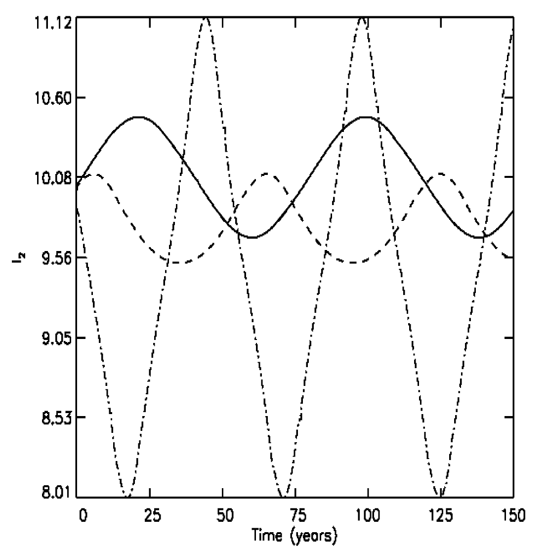
Figure 1 ††margin: FIG. 1 illustrates an asteroid’s motion with initial AU, , and , with . Direct comparison of our plots with Winter and Murray (1997)’s Figure 14 reveal nearly equivalent profiles for the evolution of orbital elements. Differences in evolution and the presence of small modulation may be attributed to the different coordinate systems in which the asteroids evolved. Varying the asteroid’s semimajor axis by an amount comparable to the barycentric correction indeed induces drastically different behavior. As to be expected in resonant systems, evolutionary behavior may be highly sensitive to the initial semimajor axes values.
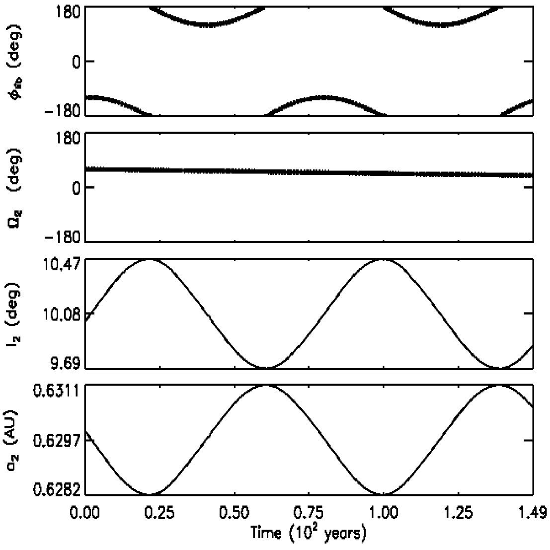
As evidenced both by observations of the Solar System and by the d’Alembert relations, one is less likely to come across a dynamical system in a purely inclination-based resonance where just one resonant angle is librating. Such a resonance must be of at least second-order, and eccentricity cannot play a role in the resonant evolution. Figure 2 ††margin: FIG. 2 illustrates an asteroid’s motion with initial AU, , and , with evolved over the same time as the asteroid in Fig. 1. Because this resonance is second-order, the so-called “strength” of the resonance scales as , as opposed to for a first-order eccentricity resonance.
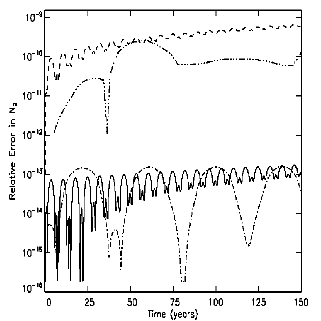
Figure 3 ††margin: FIG. 3 plots the relative error in the constants (Eq. 2.42) throughout the runs of the simulations in Figs. 1 and 2 for different user-inputted integration accuracy parameters of our code. For the eccentric asteroid in Fig. 1, the solid line results from an accuracy parameter three orders of magnitude smaller than that from the dashed line. Similarly, for the inclined asteroid of Fig. 2, the dot-dashed and dot-dot-dot-dashed lines in Fig. 3 result from accuracy parameters which differ by three orders of magnitude. Figure 3 corroborates the validity of the expression for , and exhibits variation according only to computer precision. The relative error in the constant, heliocentric Hamiltonian (Eq. 2.22), Jacobi Hamiltonian (Eq. 2.27), heliocentric constant (Eq. 2.44), Jacobi constant (Eq. 2.45), and angular momentum constants (Eqs. 2.19-2.21) are all either indistinguishable from zero or are not applicable to this specific problem.
The sole resonant argument in Figs. 1 and 2 librates about and , respectively. One may attempt to model the analytical form of the libration of resonant angles by considering Eq. (2.16). Because and vary with time, and because of the summation, the equation is not easily integrated, and the evolution of the resonant arguments are sometimes by no means simple sinusoids (see, e.g. Fig. 17a of Winter and Murray 1997). However, I find that, in some cases, the form of libration profiles can be Fourier decomposed into the dominant frequencies of the system such that
| (3.1) |
where the summation can be taken to infinity.
For example, the dominant frequency of the asteroid in Figs. 1 and 2 correspond to periods of yr and yr, as can be evidenced by considering the values from Table Figure and Table Captions††margin: TABLE 1 . This table provides a list of the coefficients, and their standard deviations, obtained by fitting Eq. (3.1) to the libration profiles from Figs. 1 and 2. I performed the fits by using the Levenberg-Marquardt algorithm (Press et al., 1992). We note also that the tiny standard deviations associated with the values indicate excellent agreement with the evolution from our code. As more Fourier terms are included, the fit becomes better, although the number of terms needed in some cases may be prohibitive. The fit to the libration profile for the inclined asteroid is significantly better than that for the eccentric asteroid when comparing the ranges ( vs. ) and standard deviations ( vs. ) of the residuals. The reason for the discrepancy has to do with the different shapes of the libration profiles.
The shape of some libration profiles suggest a better equation to fit with fewer terms. Such profiles often resemble those seen in radar Doppler velocity curves for exoplanet searches. Further, the computation of the evolution of the true anomaly from the eccentric anomaly (see Eq. 6.11) suggests that one can fit a libration profile to the following equation:
| (3.2) |
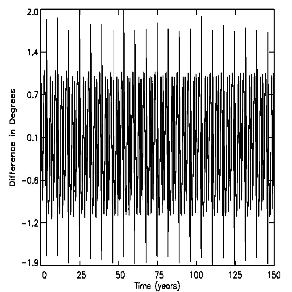
Table Figure and Table Captions ††margin: TABLE 2 provides values for this equation’s fit to the libration profiles in Figs. 1 and 2. The fit to the libration profile for the eccentric asteroid is a marked (one order of magnitude) improvement over the Fourier fit. Figure 4 ††margin: FIG. 4 displays the residuals of the new fit, and the residuals have a range of and a standard deviation of .
4 Multiple-term Systems
A disturbing function composed of just one resonant argument is often too simple a model for a realistic approximation to the evolution of bodies in a known resonance. Including the relevant secular terms may improve the approximation significantly, even though with added terms the constants of motion derived in Eqs. (2.42)-(2.45) strictly no longer exist. Orbit-orbit resonances typically involve disturbing functions with more than one resonant argument. In this case, when no secular arguments are considered, the Hamiltonian can be expressed as an appropriate linear combination of either and , or and . Hence, the other four actions are constants and can be combined to reproduce Eqs. (2.44) or (2.45). In this regime, Eqs. (2.42) and (2.43) no longer represent constants of the motion. In the more general case, where multiple resonant and secular arguments dominate the motion, the Hamiltonian and total angular momentum of the system are the only constants guaranteed to exist.
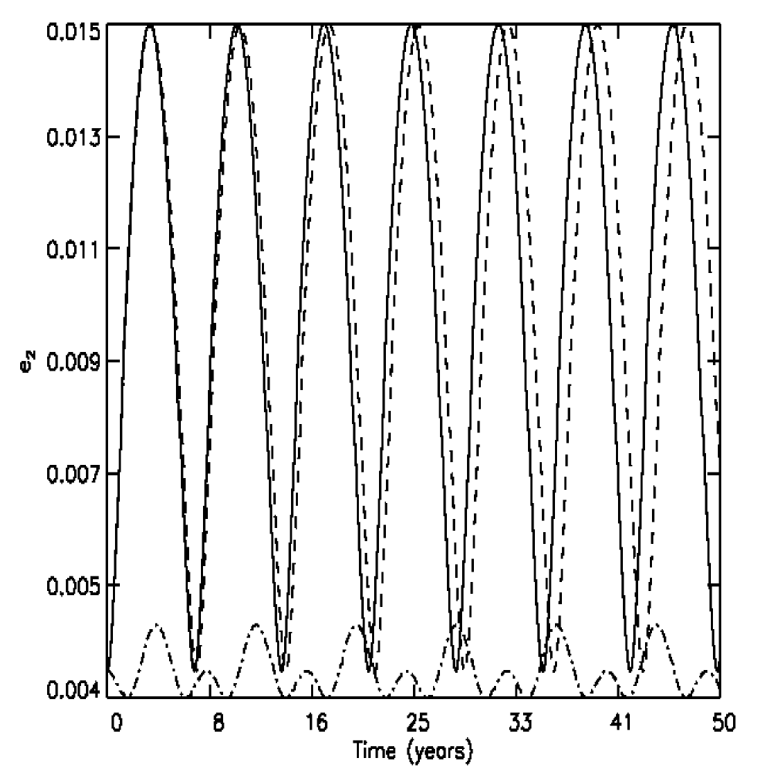
We expand our study of Jovian asteroid dynamics by including additional resonant and secular arguments, thus “perturbing” our single-term models. For the eccentric asteroid of Fig. 1 in the first-order : resonance, we now include, in Fig. 5, ††margin: FIG. 5 all terms up to second-order associated with the , and arguments (dashed line), and all terms up to fourth-order associated with the , , , , and arguments (dot-dashed line). Similarly, for the inclined asteroid of Fig. 2 in the second-order : resonance, we now include, in Fig. 6, ††margin: FIG. 6 all terms up to second-order associated with the and arguments (dashed line), and all terms up to fourth-order associated with the , , and arguments (dot-dashed line). The d’Alembert relations preclude the existence of the argument.
These figures demonstrate that the eccentricity and inclination profiles change significantly depending on the order of the terms included, even for the circular restricted three-body problem. Veras (2007) demonstrates the additional consequences of eliminating the assumption that Jupiter remains on a circular orbit. Doing so places doubt on the validity of approximating the system by a single or a few terms.
Multiple-planet systems said to be in resonance often feature one or more librating angles. The smaller the amplitude of these librating angles, the “deeper” into resonance the system is purported to be. Our model can make quantitative statements about how the depth of resonance varies with orbital parameters, and how these variations differ across different types of resonances. Here we sample phase space for regimes which could be applicable to two-planet extrasolar planetary systems. As a three-body problem, these systems are not likely to be restricted in many ways. However, one such restriction which we assume is that planets in these systems are coplanar.
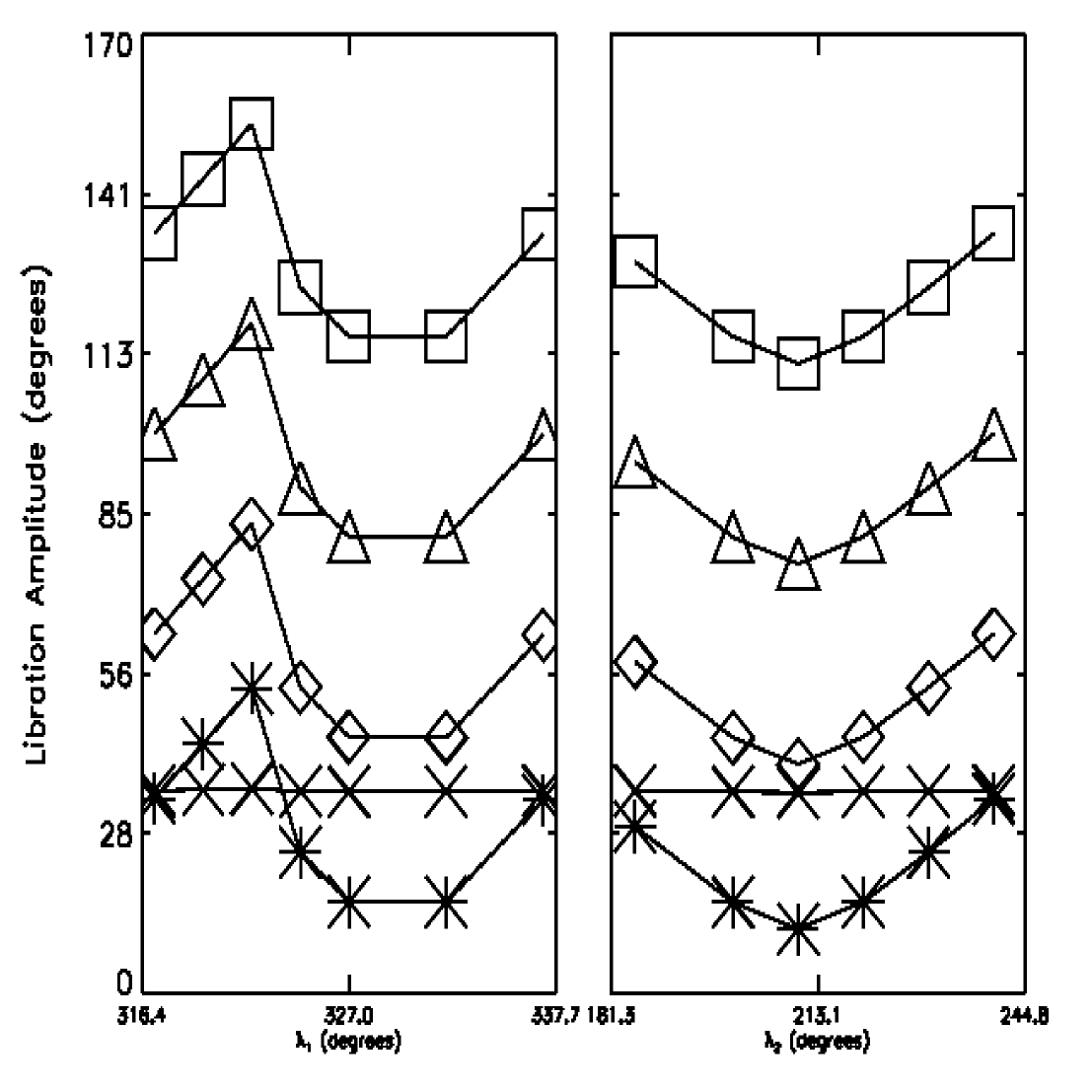
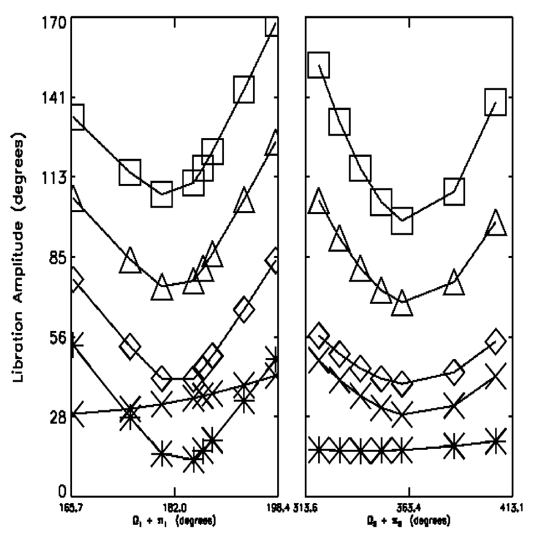
Given the extensive investigations of the : resonance, and the investigation performed in Section 5 of this work, here we sample phase space for a couple other relevant resonances: the first-order :, and third-order : resonances. For each, we have discovered configurations in the relatively small region of phase space which allows for libration of multiple arguments. The inner planet has a mass of ( Mass of Saturn) and is set at AU away from a Solar-mass star. The outer planet in the : resonant system has the same Saturn-like mass, while the outer planet in the : system is given a mass of . Table Figure and Table Captions ††margin: TABLE 3 displays the “nominal” orbital configurations from which variations result in Figs. 7 - 10. ††margin: FIG. 7 ††margin: FIG. 8 ††margin: FIG. 9 ††margin: FIG. 10 The vastness of phase space allow us to sample just a small slice, presented below, and force us to defer further analysis to future studies.
These figures plot “libration amplitude,” defined as half of the range of a resonant angle taken over a few periods. We must state such a definition because the actual evolution of these angles is sometimes heavily modulated and departs from a sinusoid, as in the dot-dashed profile from Fig. 5. Angles are said to circulate if they span , and do so for the vast majority of phase space. Each large plot symbol represents the outcome of a different simulation, and the curves which are fit through these symbols hence represent just an approximation to the shapes of these profiles. Figure 7 plots the outcomes for the : resonance, while Figs. 8-10 plot the outcomes for the : resonance. For the : resonance, asterisks and diamonds denote, respectively, the libration amplitude of the and arguments. For the : resonance, crosses, squares, triangles, diamonds and asterisks, denote, respectively, the libration amplitude of the , , , and arguments.
Dashed lines in Figs. 7-8 represent the “nominal” resonant semimajor axes. For both resonances, this value proves to be an excellent predictor for maximum depth for nearly all resonance angles. Note, however, the order-of-magnitude difference in values plotted in the two figures due to the difference in order of the resonance. The effective “libration centers,” which represent the mean value of libration, hover around and , respectively, for the asterisks and diamonds in Fig. 7. For Figs. 8-10, the libration centers are for the asterisks, crosses and triangles, and for the diamonds and squares. We don’t present plots for the variation of and for the : resonance because these variations produce differences in libration widths of less than a degree.
One can glean other results from the figures. A comparison the vertical axes reveal that in no case does a : resonant angle librate with an amplitude of less than , in stark contrast to the : resonance. This phenomenon most likely results from the difference in mass of the outer planet in the two systems; the more massive both resonant objects are, the shallower the resonance. Also, Figs. 8-10 suggest that multiple resonant arguments librate simultaneously for most of the phase space sampled, although occasionally some of the arguments circulate. Further, the curves drawn through the asterisks indicate that the libration width profiles can very drastically for different librating angles in the same system. Figure 10 demonstrates that in order to produce similar libration amplitude variations, had to be varied by a factor of three greater than did.
5 Dominant GJ 876 Terms
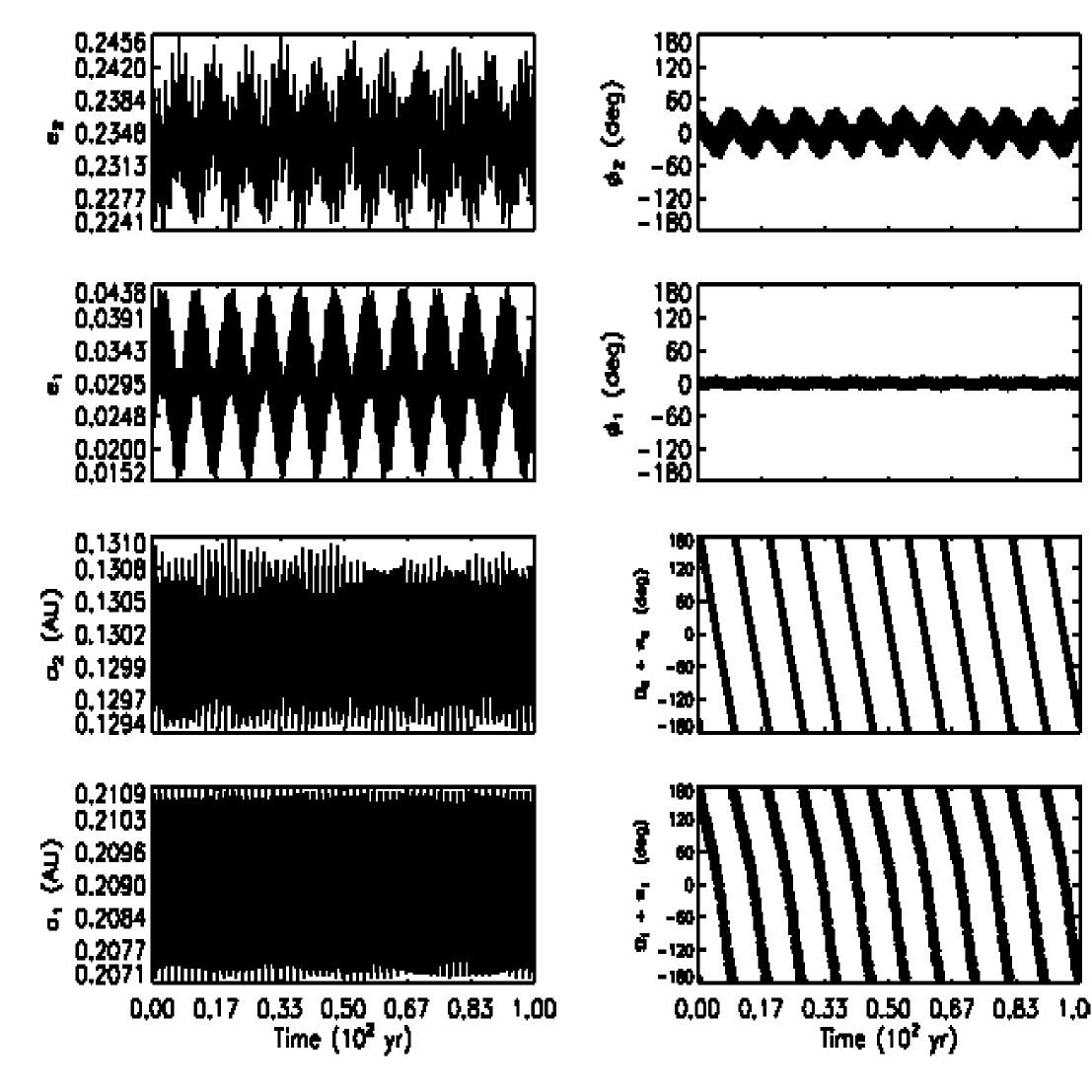
We now consider the GJ 876 system with the outer (GJ 876 b) and inner (GJ 876 c) giant planets, which are thought to reside in a : resonance. Ever improving orbital fits for initial system conditions abound; different sets may be found in Fischer et al. (2003), Laughlin et al. (2005), Rivera et al. (2005) and the on-line Extrasolar Planets Encyclopedia444 at http://vo.obspm.fr/exoplanetes/encyclo/catalog.php. We chose , , , AU, AU, , , , , , and for the numerical integration. The small circularized non-resonant planet GJ 876 d, at AU, does not significantly affect the resonant evolution of the other two planets 555We have performed a full N-body simulation with HNBody (Rauch and Hamilton 2007, in preparation) which demonstrates that the presence of planet GJ 876 d indeed has a negligible effect.. We evolve the resonant planets on coplanar orbits, and thereby neglect the inclinations and longitude of ascending nodes.
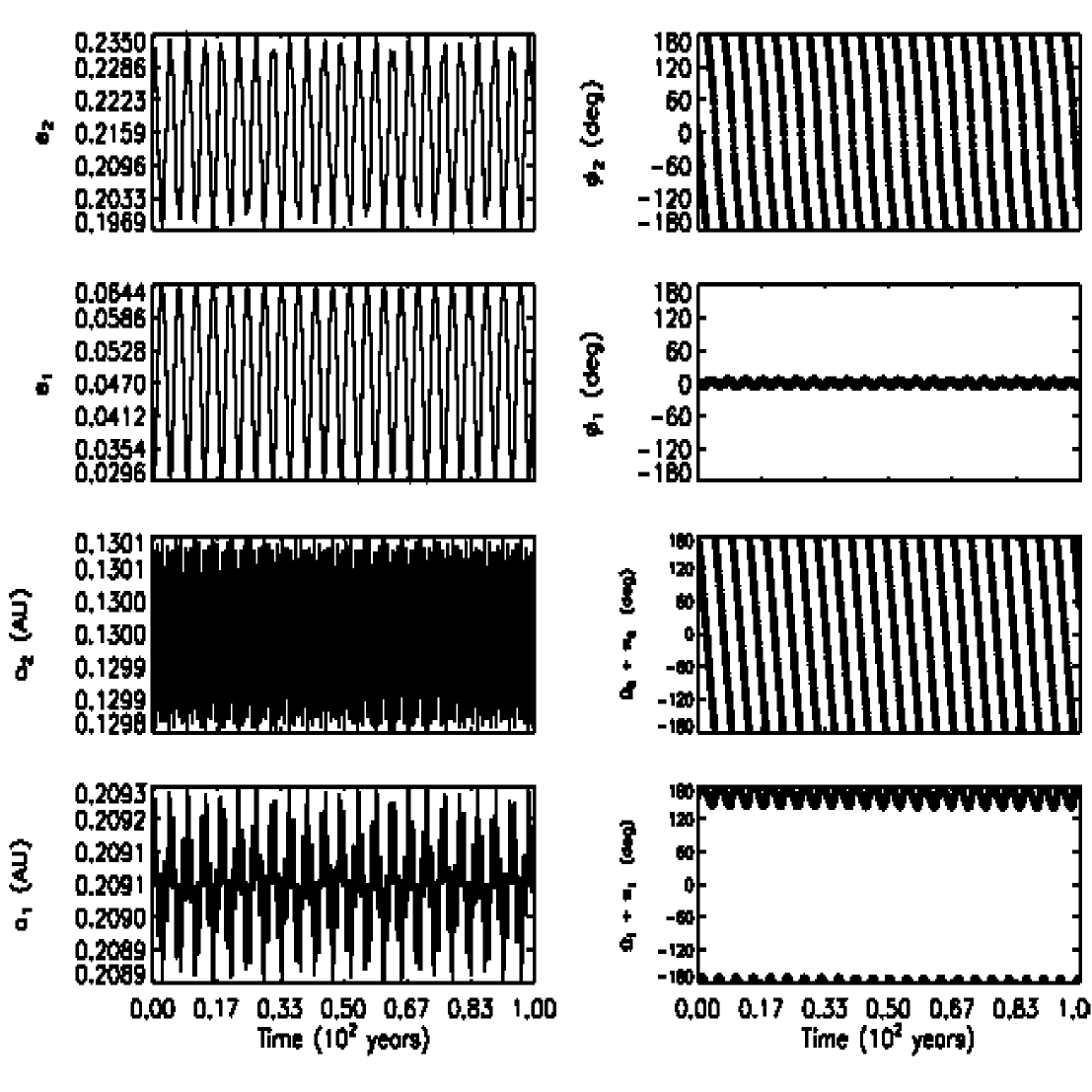
Figure 11 ††margin: FIG. 11 illustrates how the resonant planets’ orbital parameters evolve using the full N-body integrator, HNbody (Rauch and Hamilton 2007, in preparation). We define as the resonant angle corresponding to the constants , and as the resonant angle corresponding to . Figure 1 demonstrates that both and librate about , and and circulate, all with a period of years. The eccentricities exhibit a periodicity commensurate with that of the orbital angles’ amplitudes of libration, whereas the semimajor axes exhibit little (% - %) variation. The influence of the short-period terms are seen through the small modulations (or the noise) especially apparent in the orbital elements of GJ 876 c because of its relatively large eccentricity. The planets are said to be “in resonance” because of the simultaneous libration of and , and GJ 876 c is said to be in “deep resonance” because of the small () amplitude of .
A full treatment of the GJ 876 system, even to first-order in eccentricities, requires multiple resonant and secular arguments. Table Figure and Table Captions ††margin: TABLE 4 lists all relevant resonant and secular terms for this system up to fourth order, and Figs. 12-15 illustrate the planetary evolution caused by all terms up to order one, two, three and four respectively. Differences from the true evolution exhibited by Fig. 11 may be attributed to the neglect of short-period terms and even higher-order resonant and secular terms. The simulations in Figs. 12-15 were initialized with mean orbital element values, obtained from averaging over the orbital evolution of a few periods of the outer planet from the exact numerical integration. The mean initial values used were AU, AU, , , , , , and .
Figure 12 ††margin: FIG. 12 demonstrates that a full first-order treatment, which includes the leading terms from the , , and arguments, forces to circulate rather than librate and to librate about rather than circulate. These features are at odds with the full N-body integration. Therefore, analytical manipulations of these terms alone have limited utility when one attempts to analyze particular aspects of the system’s evolution.
The combination of terms comprising the second-order solution showcased in Fig. 13 ††margin: FIG. 13 is only marginally stable, and only for a high integration accuracy parameter (). Nevertheless, amidst the chaos, both and do librate about , but on a longer timescale (note difference in axes). Short-term evolution, however, showcases fictitious asymmetric libration of varying amplitude about or . The switch between both libration centers occurs at extrema of the semimajor axes and eccentricities, and the presence of asymmetric libration centers demonstrates that the first-order solution is more accurate than the second-order solution. Similar results may be found in the restricted 3-body problem (Beaugé, 1994) even though that problem is inherently different. Further, Lemaître and Henrard (1988) discuss the incorrect qualitative behavior which arises from improper truncation of the disturbing function as applied to asteroid studies.
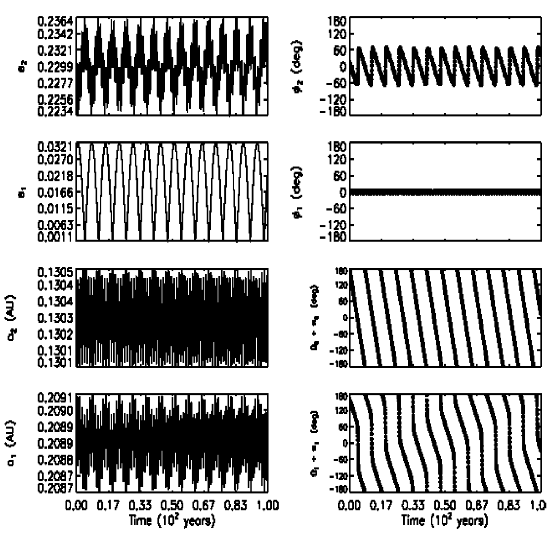
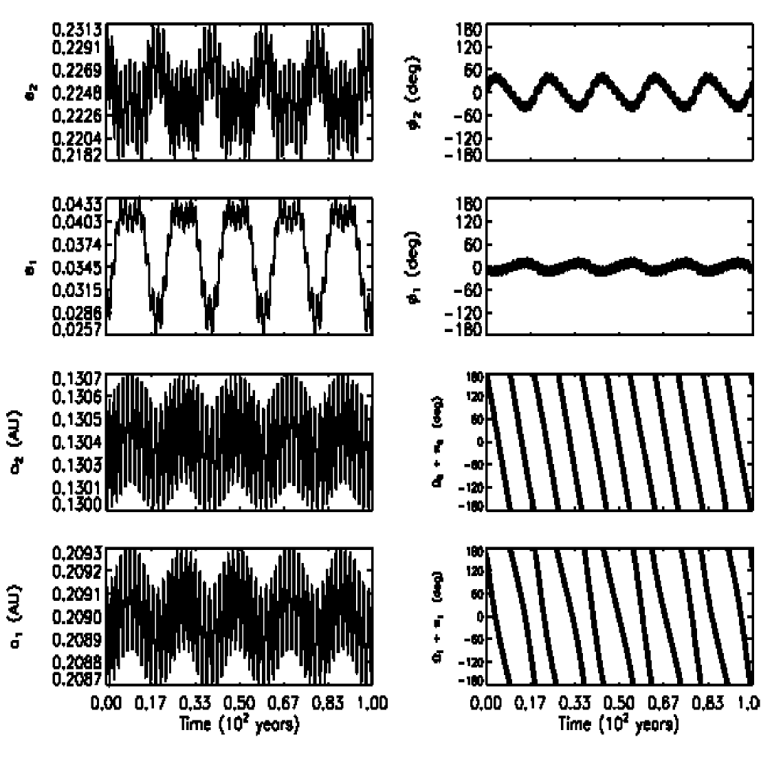
Higher-order treatments, however, not only are stable but reproduce expected features of the system. The third-order solution in Fig. 14 ††margin: FIG. 14 and the fourth-order solution in Fig. 15 ††margin: FIG. 15 reproduce, to varying extents, the orbital evolution shown from the N-body simulation of Fig. 11. However, in Fig. 14, represents an unmodulated sinusoid, lacks any modulated envelope, and acquires a slight sawtooth form. These minor features all differ from the N-body integration, but are all partially remedied by the fourth-order treatment in Fig. 15. However, this same fourth-order treatment demonstrates a decrease in precision by altering the amplitudes and elongating the libration period by over a factor of two.
The above considerations suggest that the so-called “Laplacian expansion” (described in Ellis and Murray 2000) expansion of the disturbing function best reproduces the evolution of GJ 876 for an eccentricity order between and . The lack of precision can be explained by the failure to satisfy the Sundman criterion (Sundman, 1916) for the coefficients of this expansion. In the planar case, the criterion is typically expressed as (Ferraz-Mello, 1994; Šidlichovský and Nesvorný, 1994):
| (5.1) |
where
| (5.2) |
such that is implicitly defined as . Applying the criterion to representative GJ 876 orbital parameters yields Fig. 16, ††margin: FIG. 16 which demonstrates that the classic expansion will show signs of divergence at particular points in the evolution. As more resonant terms are included, the effect of this divergence might be amplified. Hence, the optimal order with which to model GJ 876 with this expansion is finite. Taken as a sequence, Figs. 12-15 demonstrate that perhaps “order” is an inappropriate metric for classifying the accuracy of a model for systems with a phase space similar to that of GJ 876. We highlight these perturbative issues in order to caution future investigators regarding the validity of using particular resonant arguments for analytical considerations.
Resonant systems may be affected, or even dominated, by perturbations external to the detailed dynamical interplay described so far. The next three sections will present potentials for different types of perturbations and estimate their effect on GJ 876. Table Figure and Table Captions ††margin: TABLE 5 summarizes these effects and what orbital parameters they directly affect depending on the assumptions used.
6 Central Body Oblateness
6.1 Overview
The contribution of oblateness from a central body to a resonant system has shown to play a crucial role in ring and small satellite dynamics. Goździewski and Maciejewski (1998) and Shinkin (2001) have created analytical models for the dynamical evolution of satellites around oblate planets, and Wiesel (1982) has created a model of rings in resonance with an oblate planet. In this section, we incorporate the oblateness effect through both an averaged (over short-period terms) and unaveraged oblateness potential. Doing so helps determine specifically the error incurred when using the averaging approximation, and helps clarify the seemingly contradictory expressions found in the literature. The oblateness potential, , has the form,
| (6.1) |
where is the equatorial radius of the central object, are the oblateness coefficients, are Legendre polynomials, and is the declination with respect to the central object’s equatorial plane (Brouwer and Clemence, 1961, p. 563). In order to maintain consistency with the other equations in this work, we wish to express Eq. (6.1) in terms of contact elements. However, we may instead use expressions for osculating elements because every term in the expansion for the potential depends only upon the resonant body positions, and not velocities (expressions for positions are identical in both osculating and contact elements).
6.2 Averaged expressions
Various different expressions for the orbital average of the oblateness potential have appeared in the literature due to differences in meaning of the orbital elements. Greenberg (1981) attempted to eliminate the confusion regarding these seemingly dissimilar formulas. He wrote the following expressions for apsidal precession rates in osculating (subscript “o”), sidereal (subscript “s”), and epicyclic (subscript “e”) coordinates:
| (6.2) |
| (6.3) |
| (6.4) |
Any one of Eqs. (6.2)-(6.4) may be correct depending on the context of the system studied. Equation (6.2) (Brouwer, 1959) may be used when the orbital elements considered are all osculating Keplerian elements. Equation (6.3) (Brouwer, 1946; Murray and Dermott, 1999, p. 270) may be used when dealing with observed values for the sidereal mean motion and the mean distance from the central object (also called the “observed semimajor axis,” “apparent semimajor axis,” or “geometric semimajor axis”). Equation (6.4) (Elliot et al., 1981; Elliot and Nicholson, 1984; Borderies-Rappaport and Longaretti, 1994; Murray and Dermott, 1999, p. 269) may be used when the only measured orbital element is the distance from the central object, a typical characteristic of ring systems.
Our model does not utilize truncated expressions for apsidal precession. Rather, we wish to obtain an averaged disturbing function in terms of osculating elements. Unfortunately, differing expressions for averaged potentials have also appeared in the literature. Therefore, understanding the manner in which Eqs. (6.2)-(6.4) are derived from disturbing functions is important in determining the correct form of the averaged potential.
Murray and Dermott (1999, p. 269) and Métris (1991) write expressions for averaged potentials which contain a term. As the potential is a linear combination of terms, averaging only over the “fast” angle known as the true anomaly would not produce a product of the oblateness terms from which a term could be derived. Typically, terms appear in the derivations of the variation of the orbital elements. Such derivations include binomial expansions (Brouwer, 1946; Greenberg, 1981), Poincaré-von Zeipel transformations (Brouwer, 1959; Kozai, 1962), Taylor expansions of orbital elements (Kozai, 1959), or Poincaré-Lindstedt expansions (Borderies-Rappaport and Longaretti, 1994) 666The elimination of the term in Eq. (6.4) is a chance cancellation; the Appendix of Borderies-Rappaport and Longaretti (1994) shows that the and terms, for example, do not cancel.. Métris (1991) uses the Hori-Deprit method in order to illustrate how a term may appear in the potential if an additional, different averaging in the small parameters is performed over the often-neglected short-period terms. This procedure was applied to the osculating elements in order to yield the mean osculating ones. Métris’s (1991) resulting expression for differs from that of Murray and Dermott (1999, p. 269).
Further, the expression from Murray and Dermott (1999, p. 269) does not contain terms (which were argued to be typically negligible), nor terms which are independent of eccentricity or inclination. These latter terms are not constant, but rather depend on the variable semimajor axis. The terms containing vanish only if the disturbing function is averaged twice - once over the true anomaly, and once over the argument of pericenter. However, the latter orbital angle does not vary “quickly” in general.
Given the above considerations, we include Métris’ (1991) short-period terms, and use Kozai’s (1959) expression for the other terms in order to obtain an averaged potential. The resulting expression, when truncated to “fourth-order” in eccentricities and inclinations (as is the disturbing function), reads:
| (6.5) |
where,
| (6.6) |
| (6.7) |
| (6.8) |
| (6.9) |
Incorporating disturbing function partial derivatives with Eqs. (2.3) provides explicit expressions for the derivatives of the orbital elements for the oblateness contributions. In order to obtain the oblateness contribution to , one can combine the derivatives of the orbital elements with Eq. (2.2).
6.3 Complete expressions
In the unaveraged incorporation of oblateness into our model, we use Eq. (6.1) explicitly. The eccentric anomaly, , is related to the mean anomaly through Kepler’s equation:
| (6.10) |
such that .
The true anomaly is related to the eccentric anomaly through (Murray & Dermott 1999, p. 33)
| (6.11) |
Let:
| (6.12) |
Substituting Eq. (6.12) into Eq. (6.1) and then incorporating the appropriate partial derivatives into Eq. (2.3) allows us to determine the oblateness contribution for each orbital parameter. In order to compute these derivatives, the eccentric anomalies must be computed through Kepler’s Equation numerically at each timestep.
6.4 Application to GJ 876
Saturn’s oblateness dominates the precession of the pericenters of the system’s close small satellites. The Sun’s oblateness, however, despite its significance in general relativistic computations (Iorio, 2005), is thought to have a negligible effect on the evolution of the planets in the Solar System. Extrasolar systems, however, display a variety of orbital configurations which might admit the possibility of the central star’s oblateness playing a role in the evolution. Massive () planets are known to orbit their stars at distances an order of magnitude shorter than the Sun-Mercury separation, and can evolve in orbit-orbit resonances absent from the inner Solar System. We further analyze the resonant planets in GJ 876 by attempting to determine under what conditions can oblateness play a role, and how likely their evolution is affected by the property of the star. As the effect of oblateness through inspection is typically negligible, we track the contribution by explicitly plotting the contribution for the rate of change of relevant orbital elements at each timestep.
GJ 876 is an M4 dwarf with a rotational velocity similar to that of the Sun ( km/s) (Delfosse et al., 1998) and a radius just a fraction of the Sun’s (Chabrier and Baraffe, 1997). The star’s oblateness is unknown, likely changes with time, and is a detailed function of the rotation profile, mass, and radius. Rozelot et al. (2001) compares quadrupole () and octopole () Solar measurements from several references, and Rozelot and Roesch (1997) provide an upper bound to the Solar oblateness. As the range of values estimated for the Sun span two orders of magnitude (), and (Godier and Rozelot, 2000), where is the rotational velocity of the Sun, GJ 876’s oblateness is likely to fall within this range.
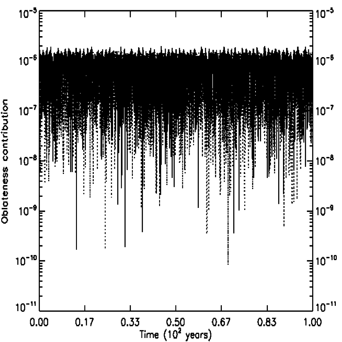
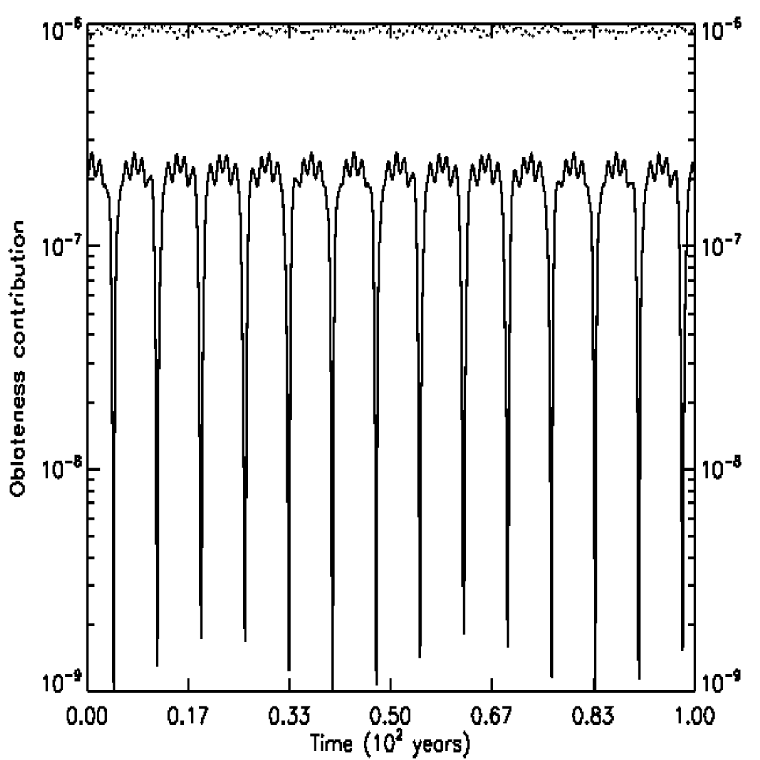
Through simulations including the 11 arguments needed for a third-order treatment, we conclude that the GJ 876 planets are negligibly affected by stellar oblateness. Figure 17 ††margin: FIG. 17 plots the fractional contribution of oblateness at each timestep of (solid line) and (dotted line) in the unaveraged planar problem given , and km; Fig. 18 ††margin: FIG. 18 is equivalent except in the averaged problem. Both figures indicate an upper bound for the fractional oblateness contribution is . The librational periodicity is more evident in Fig. 18 than Fig. 17 due to the averaged nature of the system simulated there. The magnitude of the fractional contributions from Figs 17 and 18 demonstrate that any planet nonnegligibly affected by stellar oblateness must be much closer to the central star, at a radius which is likely to be inside the tidal circularization limit.
If GJ 876 was a fast rotator ( km/s) like other observed M dwarfs (Delfosse et al. 1998), then the effect of oblateness would be at least two orders of magnitude greater, and likely affect the long-term, if not short-term, evolution of the system. As several tens of extrasolar planets have been discovered within AU of their parent stars, including several multiple systems, prospects for finding an oblate star with a tight resonant system are promising. Such stars would be Jupiter-like due to their mass, radius, and rotational period of hr.
7 Central-body Precession
7.1 Introduction
An object’s precession about its axis exerts a gravitational influence on orbiting masses. Although much precession-based research focuses on Mars’ chaotic obliquity (e.g. Hilton 1991; Groten et al. 1996; Christou and Murray 1997; Bills 1999; Bouquillon and Souchay 1999) and although occasionally general models applicable to different systems are developed (e.g. Blitzer 1984; Penna 1999), investigators of resonant systems do not always consider the effect of precession. Kozai (1960) conducted one of the first studies of how a satellite’s orbital elements are affected by the precession of its parent planet. Kinoshita (1993) studied the motion of a satellite relative to the equatorial plane of its oblate parent parent, and Rubincam (2000) discusses the possibility that Pluto may be in “precession-orbit” resonance. Expressions for the precession contribution to the disturbing function are given implicitly by Goldreich (1965b) and explicitly by Kopal (1969), Brumberg et al. (1970) and Efroimsky (2005b); using their results, we can write:
| (7.1) |
where , , and are the components of the precessional frequency corresponding to increasing moments of inertia of the central body.
7.2 Application to GJ 876
As displayed in Table 2, a central object’s precession does not alter the semimajor axes nor eccentricities of the planets directly, but rather only indirectly through . For GJ 876, we assume representative values of pHz and km. These values correspond to a precessional period of yr, which corresponds to a frequency significantly less than the mean motion of the resonant bodies, a realistic regime at least in the context of precessing stellar jets (Namouni, 2005). Figure 19 ††margin: FIG. 19 plots the fractional contribution of precession at each timestep of (solid line), (dotted line), (dashed line), and (dash-dot line). The effect on the orbital angles ranges from one part in to one part in , suggesting that for planar extrasolar planetary systems, precession may play a greater role than central-body oblateness. Direct comparison with Figs. 17-18 demonstrates the effect of precession on the evolution of and is roughly two orders of magnitude higher than that from oblateness.
8 A Surrounding Thin Disk
8.1 Introduction
The birthplace of planets and satellites, a protoplanetary or protosatellite disk ultimately determines the dynamical interactions which occur in the system. Although capture into resonance is likely to and often thought to occur after disk dissipation, and requires a dissipative medium, capture may be achieved while the disk is still present, for both protoplanetary and protosatellite disks. Thommes and Lissauer (2003) find that disks can play a crucial role in the migration and capture of planets in resonance, and Kley et al. (2004) performed numerical simulations of two planets embedded in a thin disk, and finds resonant capture to be a common occurrence.
In order to approximate the mass density profile of the nascent Solar System nebular disk, a model known as the Minimum Mass Solar Nebula (MMSN) has been devised (Weidenschilling, 1977; Hayashi, 1981). The MMSN represents the pair of values which, when inserted into the density profile, , provides the minimum nebular mass necessary to explain the current masses and positions of the planets. A variety of assumptions go into this calculation, including the fraction and location of nebular material that is eventually scattered out of the system and the possible presence and location of the snow line (Sasselov and Lecar, 2000). The commonly used MMSN prescription sets (Weidenschilling, 1977; Hayashi, 1981). 777Kuchner (2004) extended the analysis to extrasolar systems, and derived a Minimum Mass Extrasolar Nebula (MMEN) based on data from 26 exoplanets in multiple-planet systems. He derived an overall steeper profile, with , and individually fitted and values to individual multi-planet exosystems.
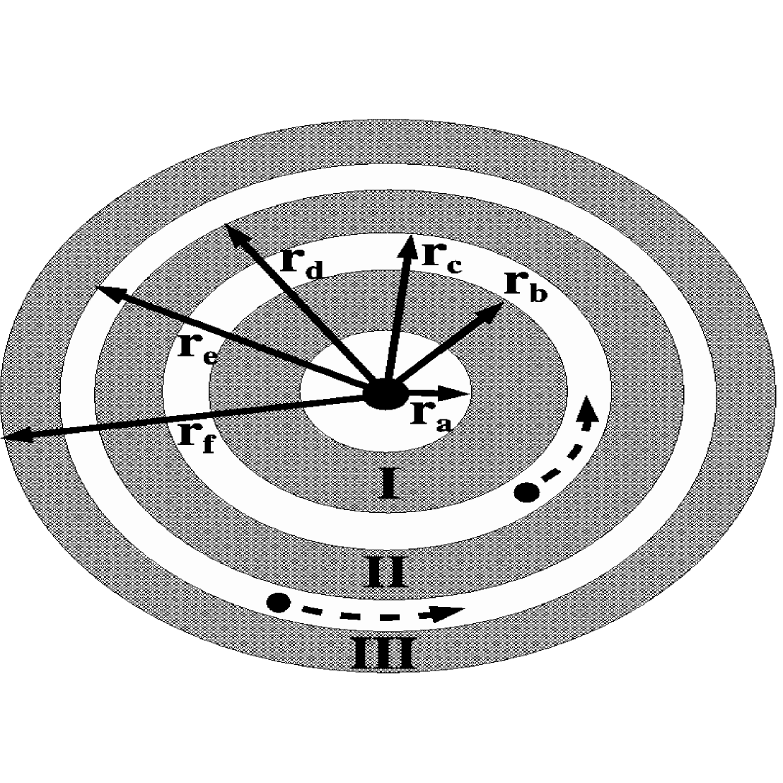
We consider only the gravity of thin steady disks with a power-law density profile , where and are constant, arbitrary parameters; we take the latter to be AU. Such profiles could represent protoplanetary or protosatellite disks. We also assume that the disk harbors two massive non-central bodies, each having already carved out a gap, as illustrated in Fig. 20. ††margin: FIG. 20 The relative sizes of the mass-filled regions labeled I, II, and III largely determine the dynamical evolution of the system. Depending on the orbital properties of planets in the system, and their interaction with the gas, regions I and II may be small or unoccupied with gas. We assume the disk contains the same total mass () as a particular fraction, , of the central mass, where
| (8.1) |
such that
| (8.2) |
8.2 Horizontal Contributions
Ballabh (1973) categorized expressions for gravitational potentials of circularly symmetric distributions of matter, in the form of homogeneous and heterogeneous disks, as polynomials in semimajor axis. Focusing on the Solar nebula, Ward (1981) computed averaged gravitational potentials due to a thin disk, and utilized Laplace coefficients in the expansions. Using the notation in the Appendix, we express the Laplace coefficients as constants. The potential at a point distance from the central body in the disk plane due to the outer (“out”) and inner (“in”) parts of a disk, read, respectively,
| (8.3) |
| (8.4) |
where and are the edges of the entire disk, and and are the boundaries of a gap that surrounds the point at which the potential is measured. Equations (8.3) and (8.4) represent just the leading-order term of the potential, not the entire potential itself. Given the schematic of Fig. 20, the disturbing functions for the outer and inner planet then become, respectively (for and ),
| (8.5) |
| (8.6) |
for fixed values of , , , , , and . At this stage we may choose to average over the angles on which and are dependent; we present both approaches for the sake of completeness. Given the derivatives of in terms of orbital elements, disturbing function derivatives can be computed directly from Eqs. (8.5)-(8.6) and incorporated into Lagrange’s planetary equations without any averaging. Conversely, expressing and in terms of orbital elements and averaging yields:
| (8.7) |
where and are functions of and , and where and are independent of and . The designations “oh” and “ih” represent “outer horizontal” and “inner horizontal.” Generalizing Eqs. (8.3)-(8.6) to admit any value of yields:
| (8.8) |
| (8.9) |
| (8.10) |
| (8.11) |
Using the binomial theorem under assumption of small yields:
| (8.12) |
| (8.13) |
With the above equations, one may now determine all of the partial derivatives of the averaged disk disturbing functions and incorporate them into Lagrange’s planetary equations.
8.3 Vertical Contributions
8.3.1 Overview
Cameron and Pine (1973) derive expressions of potential due to a cylindrical shell, but evaluate the expressions at the midplane. Ward (1981) evaluates the potential above or below the midplane by performing an inclination expansion and assuming that the maximum vertical (above the midplane) displacement of a body is much less than the distance between the disk edge and the body’s semimajor axis (). We adopt the more general assumption that , which is nearly equivalent except at high eccentricities. With this assumption, we can directly add the vertical disk contributions to the horizontal ones. In the expansion of the vertical disk contribution, the first term is independent of inclination and equals the corresponding horizontal term exactly. The next term in the expansion is of order and is incorporated into our model.
The vertical disk contribution is computed along similar lines as for the horizontal contribution, except the outer and inner potentials now read,
| (8.14) |
| (8.15) |
where as previously stated, , and is the true anomaly. These expressions represent the leading order of the portion of the potential which contains inclination. Note importantly that the summations begin with , as opposed to those from Eqs. (8.3)-(8.4). Given the expressions for the disturbing functions similar to those in Eqs. (8.5) and (8.6), and the derivatives of , , and in terms of orbital elements, disturbing function derivatives can be incorporated into Lagrange’s planetary equations without any averaging. Conversely, the averaged potential reads, with “ov” and “iv” referring to “outer vertical” and “inner vertical,”
| (8.16) |
with,
| (8.17) |
| (8.18) |
| (8.19) |
| (8.20) |
and,
| (8.21) |
| (8.22) |
8.4 Application to GJ 876
Due to the close sweeping orbits of the two resonant planets in GJ 876 and their proximity to the star, we consider only a disk exterior to the outer planet (, , so that only the region labeled “III” exists). The presence of the “common gap” in between the planets has been shown to be the result of some numerical simulations of two planets and a disk (Bryden et al., 2000; Kley, 2000). An exterior disk could represent the equilibrium state remnant from the last instance of giant planet migration. Because an accurate treatment of the short-period variations of the planetary semimajor axes and eccentricities would entail the inclusion of Lindblad and corotation resonances for disk feedback, we focus just on the disk-induced variations of the resonant angles. We take AU and AU, but through additional simulations find that the results are robust against the value of , as little mass resides toward the outer disk edge for . The value of was chosen to lie several Hill Radii away from the apocenter of the outer planet. As the disk theory presented here is viable to third order, all 11 resonant and secular arguments up to third-order were included in the disk simulations.
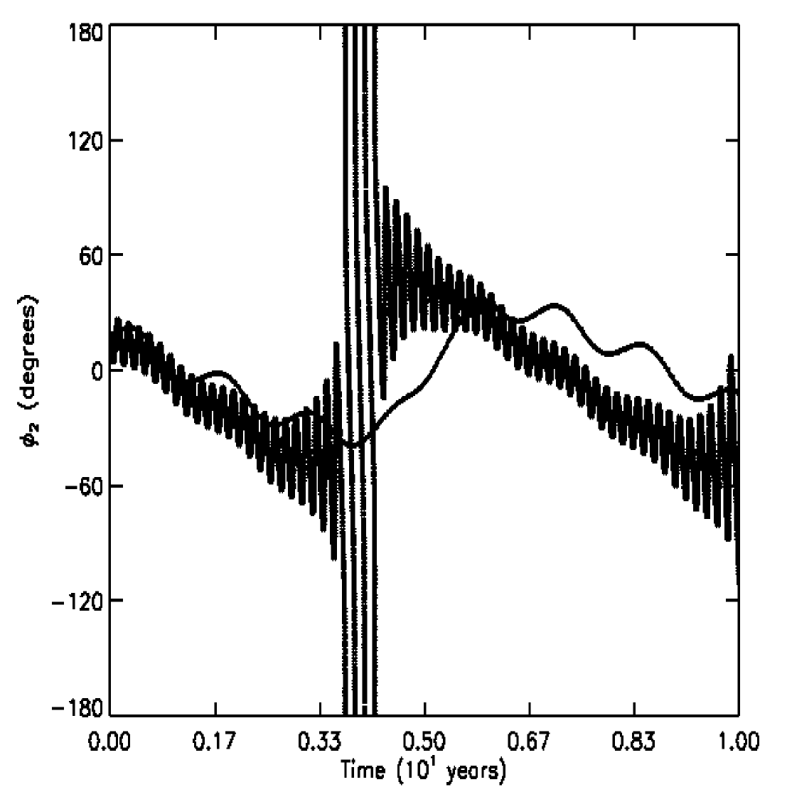
We find that disks as massive as the MMSN alters libration widths of the dominant resonant angles on the order of degrees and the circulation rates of the planets’ longitude of pericenters on the order of degrees per year. The steeper the surface density profile, the greater the effect. Most disks perturb the planetary system enough to markedly affect the orbital angle values, but not enough to change their character. However, a massive or steep enough disk will warp the profiles and transform libration into circulation. Figure 21 ††margin: FIG. 21 demonstrates how this phenomenon occurs with , , AU and AU. The background line represents the evolution of without a disk present, and the foreground crosses were computed for the presence of a disk. Of further note is that the averaged disk problem fails to reproduce this circulation. The circulation is achieved by the increase in amplitude of the short-term oscillations in the modulated envelope at almost yrs into the orbit, and repeats with subsequent librational periods.
As , and hence ultimately , a direct relationship exists between disk mass and the prospects for transforming libration into circulation. Equations (2.4), (2.12g) and (2.13e) indicate that and Eqs. (2.9) suggest . Hence, over time, as the disk primarily loses mass to the central star, the effect on apsidal libration is muted, and significant qualitative changes in apsidal behavior become more unlikely. However, transfer of disk material to either or both resonant bodies might maintain a significant perturbation on the apsidal angle. Detailed explorations of the phase space of regimes of mass loss with respect to apsidal libration represents a possible future avenue of study.
9 Conclusion
We present a model which evolves any two objects in resonance, whose orbits don’t cross, using only the resonant and secular argument defined by the user, and, optionally, including central-body oblateness, central-body precession, and the presence of a surrounding nascent disk. Many careful studies of particular resonances rely on assumptions about what aspects of a system are relevant and necessary for inclusion. Our model provides a useful tool for determining quantitative estimates of the contributions from each argument and effect, and helps determine what must or should be included when analytically studying an orbit-orbit resonance. We also provide libration width analyses of relevant regions of phase space (Figs. 7-10), general explicit expressions for the variation of each resonant or secular argument considered (Eqs. 2.16-2.18), constants of resonant motion entirely in terms of orbital elements (Eqs. 2.22, 2.42-2.44), averaged oblateness potential terms that were previously a source of confusion in the literature (Eqs. 6.5-6.9), and gap-ridden disk potentials entirely in terms of orbital elements (Eqs. 8.7-8.13 and 8.16-8.22).
We apply several aspects of this model to the GJ 876 extrasolar planetary system, and conclude that at least a third-order treatment is necessary in order to mimic the qualitative evolution of the system. A fourth-order treatment improves the approximation in some but not all respects due to Sundman’s convergence criteria for Laplacian expansions, bringing into question the viability of using “order” as the metric for quantifying the accuracy of a resonant system. The GJ 876 planets are negligibly influenced by the oblateness and precession of the central star, but suggest that given the right conditions in other exosystems, these effects may play a role in the dynamical evolution. A protoplanetary disk varies, sometimes significantly, librational amplitudes and circulation rates of extrasolar systems, and may even convert one type of motion into another. Such dynamical flags may constrain unknown orbital parameters in newly discovered exosystems.
Appendix A Appendix
The quantity (Eq. 2.10) is a function of both semimajor axes through the Laplace coefficients, . When expressed as an infinite hypergeometric series, the coefficients may be expressed as, for , (Brouwer and Clemence 1961, p. 495; Murray and Dermott 1999, p. 237):
| (A.1) |
such that
| (A.2) |
For the case of we can better compute the coefficients by using the following formula:
| (A.3) |
with .
By expressing as a polynomial in , we can then take the necessary analytical partial derivatives of and avoid integration when computing Laplace coefficients. The differential operator acts on such that for th-order eccentricity-type resonances,
| (A.4) |
where represents the function of corresponding to the particular term in the resonance which may be read off from Appendix B of Murray and Dermott (1999). The term in square brackets equals unity when . For each value of , the corresponding coefficient of may be computed. For inclination resonances, we also need to compute:
| (A.5) |
where is a counter for the linear combination of up to terms which may appear in the expression for a given inclination term (for example, ). Similarly, we have:
| (A.6) |
We can finally express , for a particular term, as:
| (A.7) |
Acknowledgments
I wish to thank Michael Efroimsky, Cristián Beaugé, Alessandro Morbidelli and an anonymous referee for valuable guidance and advice, my advisor Phil Armitage for affording me the time to pursue this endeavor and for reviewing the manuscript, Larry Esposito, Glen Stewart, and the rest of the Colorado Rings Group for their constant support, David Nesvorný for introducing me to the Sundman criterion, James Meiss and the Dynamical Systems Group for entertaining my idea, Juri Toomre for reading the manuscript, and Re’em Sari for a beneficial discussion. I gratefully acknowledge support from the National Science Foundation under grant AST 0407040, and from NASA under grant NAG5-13207 issued through the Office of Space Science.
References
- Ballabh (1973) Ballabh, G. M.: Potential Energy of Gravitationally Interacting Disk Galaxies. APSS 24, 535–561 (1973)
- Beaugé (1994) Beaugé, C.: Asymmetric librations in exterior resonances. Celestial Mechanics and Dynamical Astronomy 60, 225–248 (1994)
- Beaugé and Michtchenko (2003) Beaugé, C., Michtchenko, T. A.: Modelling the high-eccentricity planetary three-body problem. Application to the GJ876 planetary system. MNRAS 341, 760–770 (2003)
- Beaugé et al. (2006) Beaugé, C., Michtchenko, T. A., Ferraz-Mello, S.: Planetary migration and extrasolar planets in the 2/1 mean-motion resonance. MNRAS 365, 1160–1170 (2006)
- Biasco and Chierchia (2002) Biasco, L., Chierchia, L.: Effective Hamiltonian for the D’Alembert Planetary Model Near a Spin/Orbit Resonance. Celestial Mechanics and Dynamical Astronomy 83, 223–237 (2002)
- Bills (1999) Bills, B. G.: Obliquity-oblateness feedback on Mars. JGR 104, 30773–30797 (1999)
- Blitzer (1984) Blitzer, L.: Precession dynamics in spin-orbit coupling - A unified theory. Celestial Mechanics 32, 355–364 (1984)
- Borderies-Rappaport and Longaretti (1994) Borderies-Rappaport, N., Longaretti, P.-Y.: Test particle motion around an oblate planet. Icarus 107, 129–141 (1994)
- Bouquillon and Souchay (1999) Bouquillon, S., Souchay, J.: Precise modeling of the precession-nutation of Mars. A&A 345, 282–297 (1999)
- Brouwer (1946) Brouwer, D.: The motion of a particle with negligible mass under the gravitational attraction of a spheroid. AJ 51, 223–231 (1946)
- Brouwer (1959) Brouwer, D.: Solution of the problem of artificial satellite theory without drag. AJ 64, 378–397 (1959)
- Brouwer and Clemence (1961) Brouwer, D., Clemence, G. M.: Methods of Celestial Mechanics. New York: Academic Press (1961)
- Brumberg et al. (1970) Brumberg, V. A., Evdokimova, L. S., Kochina, N. G.: Analytical Methods for the Orbits of Artificial Satellites of the Moon. Celestial Mechanics 3, 197–221 (1970)
- Bryden et al. (2000) Bryden, G., Różyczka, M., Lin, D. N. C., Bodenheimer, P.: On the Interaction between Protoplanets and Protostellar Disks. ApJ 540, 1091–1101 (2000)
- Burns et al. (1985) Burns, J. A., Schaffer, L. E., Greenberg, R. J., Showalter, M. R.: Lorentz resonances and the structure of the Jovian ring. Nature 316, 115–119 (1985)
- Burns et al. (2004) Burns, J. A., Simonelli, D. P., Showalter, M. R., Hamilton, D. P., Porco, C. D., Throop, H., Esposito, L. W.: Jupiter’s ring-moon system, pp. 241–262. Jupiter. The Planet, Satellites and Magnetosphere (2004)
- Cameron and Pine (1973) Cameron, A. G. W., Pine, M. R.: Numerical models of the primitive solar nebula. Icarus 18, 377–406 (1973)
- Celletti (1993) Celletti, A.: Stability of the synchronous spin-orbit resonance by construction of librational trapping tori. Celestial Mechanics and Dynamical Astronomy 57, 325–328 (1993)
- Chabrier and Baraffe (1997) Chabrier, G., Baraffe, I.: Structure and evolution of low-mass stars. A&A 327, 1039–1053 (1997)
- Christou and Murray (1997) Christou, A. A., Murray, C. D.: A second order Laplace-Lagrange theory applied to the uranian satellite system. A&A 327, 416–427 (1997)
- Delfosse et al. (1998) Delfosse, X., Forveille, T., Mayor, M., Perrier, C., Naef, D., Queloz, D.: The closest extrasolar planet. A giant planet around the M4 dwarf GL 876. A&A 338, L67–L70 (1998)
- Efroimsky (2005a) Efroimsky, M.: Gauge Freedom in Orbital Mechanics. New York Academy Sciences Annals 1065, 346–374 (2005a)
- Efroimsky (2005b) Efroimsky, M.: Long-Term Evolution of Orbits About A Precessing Oblate Planet: 1. The Case of Uniform Precession. CeMDA 91, 75–108 (2005b)
- Efroimsky and Goldreich (2003) Efroimsky, M., Goldreich, P.: Gauge symmetry of the N-body problem in the Hamilton-Jacobi approach. Journal of Mathematical Physics pp. 5958–5977 (2003)
- Efroimsky and Goldreich (2004) Efroimsky, M., Goldreich, P.: Gauge freedom in the N-body problem of celestial mechanics. A&A 415, 1187–1199 (2004)
- Elliot et al. (1981) Elliot, J. L., French, R. G., Frogel, J. A., Elias, J. H., Mink, D. J., Liller, W.: Orbits of nine Uranian rings. AJ 86, 444–455 (1981)
- Elliot and Nicholson (1984) Elliot, J. L., Nicholson, P. D.: The rings of Uranus. In: IAU Colloq. 75: Planetary Rings (eds. Greenberg, R., Brahic, A.), pp. 25–72 (1984)
- Ellis and Murray (2000) Ellis, K. M., Murray, C. D.: The Disturbing Function in Solar System Dynamics. Icarus 147, 129–144 (2000)
- Eui Chang and Marsden (2003) Eui Chang, D., Marsden, J. E.: Geometric Derivation of the Delaunay Variables and Geometric Phases. Celestial Mechanics and Dynamical Astronomy 86, 185–208 (2003)
- Ferraz-Mello (1988) Ferraz-Mello, S.: The high-eccentricity libration of the Hildas. AJ 96, 400–408 (1988)
- Ferraz-Mello (1994) Ferraz-Mello, S.: The convergence domain of the Laplacian expansion of the disturbing function. Celestial Mechanics and Dynamical Astronomy 58, 37–52 (1994)
- Ferraz-Mello et al. (2003) Ferraz-Mello, S., Beaugé, C., Michtchenko, T. A.: Evolution of Migrating Planet Pairs in Resonance. Celestial Mechanics and Dynamical Astronomy 87, 99–112 (2003)
- Ferrer and Osacar (1994) Ferrer, S., Osacar, C.: Harrington’s Hamiltonian in the stellar problem of three bodies: Reductions, relative equilibria and bifurcations. Celestial Mechanics and Dynamical Astronomy 58, 245–275 (1994)
- Fischer et al. (2003) Fischer, D. A., Marcy, G. W., Butler, R. P., Vogt, S. S., Henry, G. W., Pourbaix, D., Walp, B., Misch, A. A., Wright, J. T.: A Planetary Companion to HD 40979 and Additional Planets Orbiting HD 12661 and HD 38529. ApJ 586, 1394–1408 (2003)
- Flynn and Saha (2005) Flynn, A. E., Saha, P.: Second-Order Perturbation Theory for Spin-Orbit Resonances. AJ 130, 295–307 (2005)
- Ford et al. (2000) Ford, E. B., Kozinsky, B., Rasio, F. A.: Secular Evolution of Hierarchical Triple Star Systems. ApJ 535, 385–401 (2000)
- Franklin and Soper (2003) Franklin, F. A., Soper, P. R.: Some Effects of Mean Motion Resonance Passage on the Relative Migration of Jupiter and Saturn. AJ 125, 2678–2691 (2003)
- Godier and Rozelot (2000) Godier, S., Rozelot, J.-P.: The solar oblateness and its relationship with the structure of the tachocline and of the Sun’s subsurface. A&A 355, 365–374 (2000)
- Goldreich (1965a) Goldreich, P.: An explanation of the frequent occurrence of commensurable mean motions in the solar system. MNRAS 130, 159–181 (1965a)
- Goldreich (1965b) Goldreich, P.: Inclination of satellite orbits about an oblate precessing planet. AJ 70, 5–9 (1965b)
- Goldreich and Peale (1966) Goldreich, P., Peale, S.: Spin-orbit coupling in the solar system. AJ 71, 425–437 (1966)
- Goździewski and Maciejewski (1998) Goździewski, K., Maciejewski, A. J.: Semi-analytical model of librations of a rigid moon orbiting an oblate planet. A&A 339, 615–622 (1998)
- Greenberg (1977) Greenberg, R.: Orbit-orbit resonances in the solar system - Varieties and similarities. Vistas in Astronomy 21, 209–239 (1977)
- Greenberg (1981) Greenberg, R.: Apsidal precession of orbits about an oblate planet. AJ 86, 912–914 (1981)
- Groten et al. (1996) Groten, E., Molodenski, S. M., Zharkov, V. N.: On the Theory of Mars’ Forced Nutation. AJ 111, 1388–1399 (1996)
- Gurfil et al. (2006) Gurfil, P., Lainey, V., Efroimsky, M.: Long-term evolution of orbits about a precessing oblate planet. 3. A semianalytical and a purely numerical approach. ArXiv Astrophysics e-prints (2006)
- Hamilton (1994) Hamilton, D. P.: A comparison of Lorentz, planetary gravitational, and satellite gravitational resonances. Icarus 109, 221–240 (1994)
- Hamilton and Burns (1993) Hamilton, D. P., Burns, J. B.: Lorentz and Gravitational Resonances on Circumplanetary Particles. Adv. Space Res. (1993)
- Harrington (1968) Harrington, R. S.: Dynamical evolution of triple stars. AJ 73, 190–194 (1968)
- Harrington (1969) Harrington, R. S.: The Stellar Three-Body Problem. Celestial Mechanics 1, 200–209 (1969)
- Hayashi (1981) Hayashi, C.: Structure of the solar nebula, growth and decay of magnetic fields and effects of magnetic and turbulent viscosities on the nebula. Progress of Theoretical Physics Supplement 70, 35–53 (1981)
- Hilton (1991) Hilton, J. L.: The motion of Mars’ pole. I - Rigid body precession and nutation. AJ 102, 1510–1527 (1991)
- Iorio (2005) Iorio, L.: On the possibility of measuring the solar oblateness and some relativistic effects from planetary ranging. A&A 433, 385–393 (2005)
- Ji et al. (2002) Ji, J., Li, G., Liu, L.: The Dynamical Simulations of the Planets Orbiting GJ 876. ApJ 572, 1041–1047 (2002)
- Ji et al. (2003) Ji, J., Liu, L., Kinoshita, H., Zhou, J., Nakai, H., Li, G.: The Librating Companions in HD 37124, HD 12661, HD 82943, 47 Ursa Majoris, and GJ 876: Alignment or Antialignment? ApJL 591, L57–L60 (2003)
- Kaula (1961) Kaula, W. M.: Analysis of Gravitational and Geometric Aspects Geodetic Utilization of Satellites. Geophysical Journal (1961)
- Kaula (1962) Kaula, W. M.: Development of the lunar and solar disturbing functions for a close satellite. AJ 67, 300–303 (1962)
- Kinoshita (1993) Kinoshita, H.: Motion of the orbital plane of a satellite due to a secular change of the obliquity of its mother planet. Celestial Mechanics and Dynamical Astronomy 57, 359–368 (1993)
- Kley (2000) Kley, W.: On the migration of a system of protoplanets. MNRAS 313, L47–L51 (2000)
- Kley et al. (2005) Kley, W., Lee, M. H., Murray, N., Peale, S. J.: Modeling the resonant planetary system GJ 876. A&A 437, 727–742 (2005)
- Kley et al. (2004) Kley, W., Peitz, J., Bryden, G.: Evolution of planetary systems in resonance. A&A 414, 735–747 (2004)
- Konacki et al. (2000) Konacki, M., Maciejewski, A. J., Wolszczan, A.: Improved Timing Formula for the PSR B1257+12 Planetary System. ApJ 544, 921–926 (2000)
- Kopal (1969) Kopal, Z.: The Precession and Nutation of Deformable Bodies, III. APSS 4, 427–458 (1969)
- Kozai (1959) Kozai, Y.: The motion of a close earth satellite. AJ 64, 367–377 (1959)
- Kozai (1960) Kozai, Y.: Effect of precession and nutation on the orbital elements of a close earth satellite. AJ 65, 621–623 (1960)
- Kozai (1962) Kozai, Y.: Secular perturbations of asteroids with high inclination and eccentricity. AJ 67, 591–598 (1962)
- Kuchner (2004) Kuchner, M. J.: A Minimum-Mass Extrasolar Nebula. ApJ 612, 1147–1151 (2004)
- Laughlin et al. (2005) Laughlin, G., Butler, R. P., Fischer, D. A., Marcy, G. W., Vogt, S. S., Wolf, A. S.: The GJ 876 Planetary System: A Progress Report. ApJ 622, 1182–1190 (2005)
- Lee (2004) Lee, M. H.: Diversity and Origin of 2:1 Orbital Resonances in Extrasolar Planetary Systems. ApJ 611, 517–527 (2004)
- Lee and Peale (2002) Lee, M. H., Peale, S. J.: Dynamics and Origin of the 2:1 Orbital Resonances of the GJ 876 Planets. ApJ 567, 596–609 (2002)
- Lee and Peale (2003) Lee, M. H., Peale, S. J.: Secular Evolution of Hierarchical Planetary Systems. ApJ 592, 1201–1216 (2003)
- Lemaître and Henrard (1988) Lemaître, A., Henrard, J.: The 3/2 resonance. Celestial Mechanics 43, 91–98 (1988)
- Ling (1991) Ling, J. F.: Application of the stroboscopic method to the stellar three-body problem. Astrophysics and Space Science 185, 51–61 (1991)
- Malhotra (1994) Malhotra, R.: Nonlinear resonances in the solar system. Physica D Nonlinear Phenomena 77, 289–304 (1994)
- Malhotra and Dermott (1990) Malhotra, R., Dermott, S. F.: The role of secondary resonances in the orbital history of Miranda. Icarus 85, 444–480 (1990)
- Marcy et al. (2001) Marcy, G. W., Butler, R. P., Fischer, D., Vogt, S. S., Lissauer, J. J., Rivera, E. J.: A Pair of Resonant Planets Orbiting GJ 876. ApJ 556, 296–301 (2001)
- Métris (1991) Métris, G.: Mean values of particular functions in the elliptic motion. Celestial Mechanics and Dynamical Astronomy 52, 79–84 (1991)
- Michtchenko and Ferraz-Mello (2001) Michtchenko, T. A., Ferraz-Mello, S.: Modeling the 5 : 2 Mean-Motion Resonance in the Jupiter-Saturn Planetary System. Icarus 149, 357–374 (2001)
- Morbidelli (2001) Morbidelli, A.: Chaotic Diffusion in Celestial Mechanics. Regular and Chaotic Dynamics (2001)
- Morbidelli (2002) Morbidelli, A.: Modern celestial mechanics : aspects of solar system dynamics. Modern celestial mechanics : aspects of solar system dynamics, by Alessandro Morbidelli. London: Taylor & Francis, 2002, ISBN 0415279399 (2002)
- Murdock (1978) Murdock, J. A.: Some mathematical aspects of spin-orbit resonance. Celestial Mechanics 18, 237–253 (1978)
- Murray and Dermott (1999) Murray, C. D., Dermott, S. F.: Solar System Dynamics. Cambridge: Cambridge University Press (1999)
- Namouni (2005) Namouni, F.: On the Origin of the Eccentricities of Extrasolar Planets. AJ 130, 280–294 (2005)
- Peale (1976) Peale, S. J.: Orbital resonances in the solar system. ARA&A 14, 215–246 (1976)
- Peale (1986) Peale, S. J.: Orbital resonances, unusual configurations and exotic rotation states among planetary satellites, pp. 159–223. IAU Colloq. 77: Some Background about Satellites (1986)
- Penna (1999) Penna, G. D.: Analytical and numerical results on the stability of a planetary precessional model. Celestial Mechanics and Dynamical Astronomy 75, 103–124 (1999)
- Press et al. (1992) Press, W. H., Teukolsky, S. A., Vetterling, W. T., Flannery, B. P.: Numerical recipes in FORTRAN. The art of scientific computing. Cambridge: University Press, c1992, 2nd ed. (1992)
- Psychoyos and Hadjidemetriou (2005) Psychoyos, D., Hadjidemetriou, J. D.: Dynamics Of 2/1 Resonant Extrasolar Systems Application to HD82943 and GLIESE876. Celestial Mechanics and Dynamical Astronomy 92, 135–156 (2005)
- Rivera et al. (2005) Rivera, E. J., Lissauer, J. J., Butler, R. P., Marcy, G. W., Vogt, S. S., Fischer, D. A., Brown, T. M., Laughlin, G., Henry, G. W.: A Planet Orbiting the Nearby Star, GJ 876. ApJ 634, 625–640 (2005)
- Roig et al. (1998) Roig, F., Simula, A., Ferraz-Mello, S., Tsuchida, M.: The high-eccentricity asymmetric expansion of the disturbing function for non-planar resonant problems. A&A 329, 339–349 (1998)
- Rozelot et al. (2001) Rozelot, J. P., Godier, S., Lefebvre, S.: On the theory of the oblateness of the Sun. Solar Physics 198, 223–240 (2001)
- Rozelot and Roesch (1997) Rozelot, J. P., Roesch, J.: An Upper Bound to the Solar Oblateness. Solar Physics 172, 11–18 (1997)
- Rubincam (2000) Rubincam, D. P.: Pluto and Charon: A case of precession-orbit resonance? JGR 105, 26745–26756 (2000)
- Sasselov and Lecar (2000) Sasselov, D. D., Lecar, M.: On the Snow Line in Dusty Protoplanetary Disks. ApJ 528, 995–998 (2000)
- Schaffer and Burns (1992) Schaffer, L., Burns, J. A.: Lorentz resonances and the vertical structure of dusty rings - Analytical and numerical results. Icarus 96, 65–84 (1992)
- Shinkin (2001) Shinkin, V. N.: Approximate Analytic Solutions of the Averaged Three-Body Problem at First-Order Resonance with Large Oblateness of the Central Planet. Celestial Mechanics and Dynamical Astronomy 79, 15–27 (2001)
- Sidlichovsky (1983) Sidlichovsky, M.: On the double averaged three-body problem. Celestial Mechanics 29, 295–305 (1983)
- Snellgrove et al. (2001) Snellgrove, M. D., Papaloizou, J. C. B., Nelson, R. P.: On disc driven inward migration of resonantly coupled planets with application to the system around GJ876. A&A 374, 1092–1099 (2001)
- Sundman (1916) Sundman, K.: Sur les conditions nécessaires et suffisantes pour la convergence du développement de la fonction perturbatrice dans le mouvement plan. Öfversigt Finska Vetenskaps-Soc. (1916)
- Thommes and Lissauer (2003) Thommes, E. W., Lissauer, J. J.: Resonant Inclination Excitation of Migrating Giant Planets. ApJ 597, 566–580 (2003)
- Šidlichovský and Nesvorný (1994) Šidlichovský, M., Nesvorný, D.: Temporary capture of grains in exterior resonances with the Earth: Planar circular restricted three-body problem with Poynting-Robertson drag. A&A 289, 972–982 (1994)
- Vakhidov (2001) Vakhidov, A. A.: Asteroid orbits in mixed resonances: some numerical experiments. P&SS 49, 793–797 (2001)
- Varadi et al. (1999) Varadi, F., Ghil, M., Kaula, W. M.: Mass-Weighted Symplectic Forms for the N-Body Problem. Celestial Mechanics and Dynamical Astronomy 72, 187–199 (1999)
- Veras (2007) Veras, D.: Dangers of Truncating the Disturbing Function In Small Body Solar System Dynamics. In: American Institute of Physics Conference Series, pp. 175–186 (2007)
- Veras and Armitage (2007) Veras, D., Armitage, P. J.: Extrasolar planetary dynamics with a generalized planar Laplace-Lagrange secular theory. ApJ 661, 1311–1322 (2007)
- Ward (1981) Ward, W. R.: Solar nebula dispersal and the stability of the planetary system. I - Scanning secular resonance theory. Icarus 47, 234–264 (1981)
- Weidenschilling (1977) Weidenschilling, S. J.: The distribution of mass in the planetary system and solar nebula. APSS 51, 153–158 (1977)
- Wiesel (1982) Wiesel, W.: Saturn’s rings - Resonance about an oblate planet. Icarus 51, 149–154 (1982)
- Winter and Murray (1997) Winter, O. C., Murray, C. D.: Resonance and chaos. I. First-order interior resonances. A&A 319, 290–304 (1997)
Figure and Table Captions
Figure 1: Evolution of a Jovian asteroid on an eccentric orbit. The resonant angle .
Figure 2: Evolution of a Jovian asteroid on an inclined orbit. The resonant angle .
Figure 3: Relative error in for the asteroid evolution in Fig. 1 for user-inputted integration accuracy parameters of (solid) and (dashed), and for the evolution in Fig. 2 for accuracy parameters of (dashed-dot) and (dashed-dot-dot-dot).
Figure 4: Deviation of the libration profile in Fig. 1 from the model of Eq. (3.2) using coefficients in Table Figure and Table Captions.
Figure 5: The eccentricity profile in Fig. 1 (solid line) and those derived with all terms up to second-order from the arguments , , and (dashed line) and with all terms up to fourth-order from the arguments , , , , and (dot-dashed line).
Figure 6: The inclination profile in Fig. 2 (solid line) and those derived with all terms up to second-order from the arguments and (dashed line) and with all terms up to fourth-order from the arguments , , and (dot-dashed line).
Figure 7: Libration amplitudes for two planets in a : resonance with parameters that vary from the state given in Table Figure and Table Captions. Diamonds and asterisks represent half the variation exhibited by the and arguments respectively for individual simulations. The dashed line indicates a “nominal” value of .
Figure 8: Libration amplitudes for two planets in a : resonance with parameters that vary from the state given in Table Figure and Table Captions. Crosses, squares, triangles, diamonds and asterisks represent half the variation exhibited by the , , , , arguments respectively for individual simulations. The dashed line indicates a “nominal” value of .
Figure 11: GJ 876 b’s and c’s evolution from a full N-body integration. The angles and undergo libration about , and and undergo circulation.
Figure 12: GJ 876 b’s and c’s evolution due to all resonant and secular terms up to first order in eccentricities.
Figure 13: GJ 876 b’s and c’s evolution due to all resonant and secular terms up to second order in eccentricities.
Figure 14: GJ 876 b’s and c’s evolution due to all resonant and secular terms up to third order in eccentricities.
Figure 15: GJ 876 b’s and c’s evolution due to all resonant and secular terms up to fourth order in eccentricities.
Figure 16: Laplacian convergence region for minimum values of and (dashed lines), maximum values of and (dash-dot lines), minimum value of and maximum value of (dotted lines), and maximum value of and minimum value of (solid lines), for eccentricity values (dots) achieved during the simulation.
Figure 17: Central-body oblateness contribution to system evolution per timestep expressed as a fraction of the unperturbed values of (solid line) and (dotted line) assuming values of , and km in the unaveraged problem.
Figure 18: Central-body oblateness contribution to system evolution per timestep expressed as a fraction of the unperturbed values of (solid line) and (dotted line) assuming values of , and km in the averaged problem.
Figure 19: Precessional contribution to system evolution per timestep expressed as a fraction of the unperturbed values of (solid line), (dotted line), (dashed line), and (dash-dot line). Values of pHz and km are assumed.
Figure 20: Cartoon of two planets embedded in a surrounding thin disk with gaps.
Figure 21: Evolution of without a disk (background curve) and with a disk (foreground crosses) that is the mass of the central star with a power law exponent of and with AU, AU. Note how the disk converts resonant libration into circulation.
Table 1: Constants and their standard deviation obtained in Eq. (3.1)’s analytical fit to the libration profile for the eccentric asteroid from Fig. 1 and the inclined asteroid from Fig. 2. The range and standard deviation of the difference between the fit and the model for the eccentric asteroid is and , and for the inclined asteroid is and .
Table 2: Constants and their standard deviations obtained in Eq. (3.2)’s analytical fit to the libration profile for the eccentric asteroid from Fig. 1 and the inclined asteroid from Fig. 2. The range and standard deviation of the difference between the fit and the model for the eccentric asteroid is and , and for the inclined asteroid is and .
Table 4: Summary of resonant and secular disturbing function cosine arguments, each of which may admit more than one term, relevant to the GJ 876 system up to fourth-order in eccentricities.
Table 5: Summary of the orbital elements directly affected () by central-body oblateness and precession, and a nascent disk, under the assumptions of orbit averaging and planarity.
Table 1
| Constants | Eccentric asteroid | Eccentric asteroid | Inclined asteroid | Inclined asteroid |
|---|---|---|---|---|
| -0.204 | 0.10 | 180 | 0.0053 | |
| 1.15 | 0.24 | 60.6 | 0.0087 | |
| 38.0 | 0.14 | 11.5 | 0.017 | |
| 0.883 | 0.000061 | 0.0805 | 0.0000028 | |
| 0.870 | 0.127 | -0.290 | 0.015 | |
| 0.041 | 0.253 | -0.556 | 0.010 | |
| 1.60 | 0.0030 | 0.238 | 0.00027 | |
| 0.0494 | 0.127 | -0.409 | 0.0077 | |
| -0.00379 | 0.25 | 0.0924 | 0.016 | |
| 3.23 | 0.051 | 0.406 | 0.00041 |
Table 2
| Constants | Eccentric asteroid | Eccentric asteroid | Inclined asteroid | Inclined asteroid |
|---|---|---|---|---|
| -0.0694 | 0.0098 | 180 | 0.014 | |
| 36.8 | 0.013 | -61.3 | 0.015 | |
| -1.56 | 0.00053 | 2.95 | 0.00039 | |
| 1.97 | 0.00047 | 2.03 | 0.00086 | |
| 2.05 | 0.0020 | 0.964 | 0.00061 | |
| 0.442 | 0.0000020 | 0.0402 | 0.0000018 |
Table 3
| Resonance | |||||||||
|---|---|---|---|---|---|---|---|---|---|
| : | 0.763 | 0.05 | 0.15 | 281 | 210 | 140 | 340 | ||
| : | 0.397 | 0.25 | 0.01 | 327 | 220 | 186.5 | 340 |
Table 4
| “resonant” (R) or “secular” (S) | argument | 1st-order | 2nd-order | 3rd-order | 4th-order |
|---|---|---|---|---|---|
| S | , | , , | |||
| S | , | ||||
| S | |||||
| R | , | ||||
| R | , | ||||
| R | , | ||||
| R | , | ||||
| R | , | ||||
| R | |||||
| R | |||||
| R | |||||
| R | |||||
| R | |||||
| R | |||||
| R | |||||
| R | |||||
| R |
Table 5
| effect: | oblateness | disk | precession | |||||||
| averaged? | yes | yes | no | no | yes | yes | no | no | no | |
| planar? | yes | no | yes | no | yes | no | yes | no | no | |