Detailed Analysis of Balmer Lines in a SDSS Sample of 90 Broad Line AGN

Abstract

In order to contribute to the general effort aiming at the improvement of our knowledge about the physical conditions within the Broad Line Region (BLR) of Active Galactic Nuclei (AGN), here we present the results achieved by our analysis of the spectral properties of a sample of 90 broad line emitting sources, collected at the Sloan Digital Sky Survey (SDSS) database. By focusing our attention mainly onto the Balmer series of hydrogen emission lines, which is the dominant feature in the optical wavelength range of many BLR spectra, we extracted several flux and profile measurements, which we related to other source properties, such as optical continuum luminosities, inferred black hole masses, and accretion rates. Using the Boltzmann Plot method to investigate the Balmer line flux ratios as a function of the line profiles, we found that broader line emitting AGN typically have larger $\rm H\alpha/H\beta$ and smaller $\rm H\gamma/H\beta$ and $\rm H\delta/H\beta$ line ratios. With the help of some recent investigations, we model the structure of the BLR and we study the influence of the accretion process on the properties of the BLR plasma.

1. Introduction

The dominant features in many Active Galactic Nuclei (AGN) spectra are broad emission lines which originate in the Broad Line Region (BLR) (Osterbrock, 1989; Krolik, 1999; Peterson, 2003). The BLR can potentially provide a useful probe of the central source, thus understanding its physics and kinematics is a crucial step in the investigation of AGN. There are three reasons: (i) the kinematics of the BLR is probably controlled by the central source, with the competing effects of gravity and radiation pressure; (ii) the BLR reprocesses the X-ray/UV energy emitted by the continuum source, consequently the broad emission lines can provide indirect information about this part of the spectrum; (iii) there is indication that the parameters of the broad lines (coming from the BLR) may be related to other fundamental properties of the source. Most of the recent BLR studies have been focused on geometries, sizes, and correlations between the BLR kinematical properties and the general characteristics of AGN (see e. g. Sulentic, Marziani, & Dultzin-Haycan, 2000; Popović et al., 2004; Kaspi et al., 2005, etc.), while other works have been devoted to reconstructing the physical conditions in the BLR emitting gas (Kaspi & Netzer, 1999; Popović, 2003, 2006; Korista & Goad, 2004; Véron-Cetty et al., 2006, etc.).

The broad line strength, width, and shape are powerful tools for gas diagnostics in the different parts of the emitting region of AGN (e. g. Osterbrock, 1989). However, there is the problem that the broad emission lines are complex and that they are probably coming from at least two regions with different kinematical and physical conditions. Furthermore, the broad emission line profiles of some AGN may be explained with a two-component model (see e. g. Popović et al., 2002, 2003, 2004; Ilić et al., 2006; Bon et al., 2006).

Here we describe an extensive investigation of the spectral properties of the broad components in the Balmer emission lines, combined with the study of those other source physical parameters that we were able to infer from our sample of spectra. Exploiting some recent results that have been achieved by means of the Reverberation Mapping (RM) technique (cfr. Kaspi et al., 2005; Bentz et al., 2006), we try to determine the central source masses and luminosities throughout the sample and to costrain their role in controlling the BLR structure and dynamics.

The paper is organized according to the following plan: in § 2 we describe the selection of our sample and we summarize the required reduction process before performing our measurements; in § 3 we report the extraction of our measurments and their related uncertainties; § 4 will list our results, with a discussion of our findings and their limits, while in § 5 our conclusions are given.

2. Sample selection and processing

The set of spectra for our data sample (see an example in Fig. 1), has been collected at the spectral database of the $3^{rd}$ data release from the SDSS. Observations are performed as survey campaigns at the 2.5m $f/5$ modified Ritchey-Chretien altitude-azimuth telescope, located at the Apache Point Observatory, New Mexico (USA). Data are obtained with a spectrograph, whose sensor uses a mosaic made up by four SITe/Tektronix 2048 x 2048 CCDs, which covers a wavelength range running from 3800Å to 9200Å. A system of 640 optical fibers, each having an aperture of 3^′′, subdivides the telescope’s field of view, so that each exposure yields 640 spectra corresponding to as many areas in the sky. The spectral resolution R of the observations ranges from 1850 to 2200. According to the purposes of our work, we searched the SDSS database for sources corresponding to the following requirements:

Figure 1.— Multiple Gaussian decomposition of the Balmer line profiles in the spectrum of SDSS J1203+0229. Here we denote with the appropriate labels all the emission lines that we took into account. The observed spectrum (thick continuous line) has been artificially shifted upwards for a better comparison with the narrow (short dashed), broad (long dashed), and Fe II (dotted) contributions. The dot-dashed line in the bottom part of each panel gives the fit residuals.

1. objects had to be located at redshift $z<0.4$, in particular it was required that the entire profiles of lines belonging to the Balmer series were covered by the available spectral range;

2. only spectra where the Balmer series was clearly recognized, at least up to the $\rm H\delta$, have been considered;

3. the profile of a broad component had to be detectable for each Balmer line;

4. such profiles had not to be affected by distortions, due, for example, to bad pixels on the sensors, as well as by the presence of strong foreground or background sources.

The preview spectra provided by the database retrieval software were manually inspected, looking for the objects in better agreement with our requirements, until a number of 115 sources were chosen from approximately 600 candidates examined in various survey areas. Subsequent inspection of the spectra collected within the database led to the rejection of 25 objects, which were affected by problems that could not be detected in the preview analysis. Therefore our resulting sample includes the spectra of 90 variously broad line emitting AGN, corresponding to $\sim 15\%$ of the candidates that we examined and located in the range $0.024\leq z\leq 0.368$, with an average redshift of 0.119. A significant fraction of our sample (45 spectra) has been selected from the collection of sources studied by Boroson (2003).

The SDSS database provides users with pre-processed material, therefore spectra retrieved from the survey are already corrected for instrumental and environmental effects, including the sky emission subtraction and the correction for telluric absorptions. Calibration of data in physical units of flux and wavelength is also performed. Consequently, our preliminary reduction simply needs to take into account a correction for Galactic Extinction, which we estimated using an empirical selective extinction function (see Cardelli, Clayton, & Mathis, 1989) that was computed for each spectrum on the basis of the Galactic Extinction coefficients given by Schlegel, Finkbeiner, & Davis (1998) and available at the Nasa Extragalactic Database (NED), and the removal of cosmological redshift. Since our interest lies on the investigation of the BLR properties, we had to identify the broad line components in spectra. In principle, the BLR signature can be isolated if we know which contributions are introduced by the underlying continuum of both the AGN and its host and by the Narrow Line Region (NLR). In many cases large samples are dealt with by means of automatic data processing techniques, which can be particularly useful in a statistical sense, but they neglect most of the peculiar properties of the single sources. In our case, intrinsic differences among the various objects certainly did not simplify the task. Broad and narrow lines, indeed, usually have blended profiles, whose final shape may critically depend on many circumstances, such as the orientation of our line of sight onto the source, the presence of absorbing material, or the amount of signal originating outside the source itself. For this reason we undertook the task of manually identifying the BLR contributions in spectra, rather than relying on automatically collected determinations. We used the IRAF software for reduction and analysis of our data. At first, we performed a continuum normalization, fitting the underlying continuum shape of each spectrum in the rest frame wavelength ranges typically running between 3750 - 3850Å, 4200 - 4250Å, 4700 - 4800Å, 5075 - 5125Å, 5600 - 5700Å, 6150 - 6250Å, and 6800 - 7000Å, which were not affected by significant line contamination. The shape of the spectral continuum was reproduced by means of spline functions with order ranging from 3 to 7 in the splot task of IRAF. As shown in Fig. 1, subtraction of the narrow line components has been achieved by means of multiple Gaussian fits to their profiles. Using the narrow [O III] feature at 5007Å, we extracted a template profile for forbidden lines in each spectrum and the other narrow lines were required to have compatible widths. The line intensity ratio for the [N II] doublet at $\lambda\lambda$ 6548, 6584 has been fixed to $1:3$. In a certain number of cases, before proceeding with our measurements of fluxes and profiles, we had to remove the contribution due to the Fe II multiplets. According to the suggestions given by Véron-Cetty, Joly, & Véron (2004), the removal of spectral contributions from Fe II can be performed by scaling and smoothing a template Fe II spectrum, which was previously extracted from the spectrum of I Zwicky 1 (Botte et al., 2004). We scaled the template according to the Fe II features seen in spectra and we measured the resulting fluxes in order to estimate the Fe II contribution. However this step was unnecessary for many objects in the sample, since the Fe II emission lines gave negligible contributions to the fluxes or they were undiscernible above the average noise intensity fluctuations in these sources.

2.1. Host galaxy correction

Figure 2.— Spectral decomposition of SDSS J1307–0036. In this plot we show the spectrum of the object in the rest frame wavelength range used to perform the fit (thick continuous line), the AGN component (thin continuous line), the host galaxy contribution (long dashed line), and the fit residuals (short dashed line).

Light from targets observed by the SDSS spectrographs is collected within sky areas of fixed aperture, which, in the case of AGN, will bring to various contributions from the host galaxy to the total flux recorded by instruments, essentially depending on the object redshift and on the relative importance of the host with respect to its AGN. A possible way to account for the influence of host galaxies on the formation of the resulting spectra is the one proposed by Vanden Berk et al. (2006) on the basis of the Karhunen-Loève Transforms described in Connolly et al. (1995). This technique assumes that the total spectrum of an AGN and its host galaxy may be the result of a sum of orthonormal components, which make up a set of eigenspectra, arranged in a linear combination such as:

$$S(\lambda)=\sum_{i=1}^{n}[a_{i}\cdot A_{i}(\lambda)]+\sum_{j=1}^{m}[h_{j}\cdot H_{j}(\lambda)],$$

where we call $S(\lambda)$, $A_{i}(\lambda)$, and $H_{j}(\lambda)$ the total spectrum, the $i^{th}$ AGN eigenspectrum, and the $j^{th}$ host galaxy eigenspectrum, while $a_{i}$ and $h_{j}$ are respectively the AGN and host galaxy eigencoefficients for the corresponding components, which do not depend on wavelength. The possibility to estimate the host galaxy contribution in the resulting spectrum stems from the use of appropriate sets of eigenspectra, like those computed by Yip et al. (2004a, b), both for galaxies and AGN, from large samples of galaxy and AGN SDSS spectra. We used an iterative $\chi^{2}$ minimization process, which was run over the rest frame wavelengths covering the range from 3700Å to 7000Å, to assign the appropriate eigencoefficient values for the decomposition of our spectra. In a similar analysis to the one performed by Vanden Berk et al. (2006), we found that most of the variations within our sample could be accounted for by introducing five galaxy and six AGN components, because a smaller number of eigenspectra left very large residuals, whilst a larger number took to a dangerous overfitting of noise fluctuations. The decomposition of our spectra usually yielded a reduced residual of $0.05<\chi^{2}<2$ in the continuum. In Fig. 2 we give an example of a spectral decomposition obtained by combining separately all the AGN and host components. The figure illustrates that this method is actually able to fit the spectral continuum in good detail, although significant residuals are left in the regions corresponding to the line cores, where the highest order variations of our sample are carried out. The spectral contributions identified as being due to the host were therefore removed from our subsequent measurments of the AGN properties and they have been used to estimate the relative importance of the AGN and its host in the emission of the observed luminosities. Fig. 3 illustrates the amount of host galaxy contaminations detected in our sample in the form of a histogram. When we studied the distribution of these non-AGN components, we found no clear evidence for a redshift or luminosity dependence. Indeed, taking into account objects at larger distances, there is a higher probability to include more powerful AGN and this may balance the effect of light collected from a wider fraction of the host.

Figure 3.— Relative importance of host galaxy contamination to the optical continuum in the spectra of our sample. The distribution does not show any particular dependence on the object redshift or its luminosity.

3. Spectral analysis

Once the broad line components had been fairly isolated in the spectra, we performed a number of measurements in order to estimate fluxes, FWHM, and FWZI. The fluxes of the Balmer lines were measured several times and the uncertainties to be associated to the line flux determinations were computed as:

$$\sigma_{F}=\sqrt{\left(\frac{\sigma_{\rm cont}}{I_{50}}\cdot F\right)^{2}+{\bar{\sigma}_{F}}^{2}},$$

where $\sigma_{\rm cont}$ represents the rms due to noise fluctuations estimated in the continuum close to the emission lines, $F$ and $I_{50}$ are, respectively, the total fluxes of the lines and their half maximum intensities, while $\bar{\sigma}_{F}$ is the standard deviation of our multiple flux determinations with different choices of the continuum intensity level. A list of flux ratios for various Balmer lines, with respect to $\rm H\beta$ from different sources, is given in Table 1. Their error bars are obtained as:

$$\sigma_{Rj}=R_{j}\cdot\sqrt{\left(\frac{\sigma_{Fj}}{F_{j}}\right)^{2}+\left(\frac{\sigma_{H\beta}}{F_{\rm H\beta}}\right)^{2}},$$

where $R_{j}$ is the ratio of $j^{th}$ Balmer line with respect to $\rm H\beta$. Similar flux measurments have been performed on the [O III] emission line at 5007Å and they are also reported in Table 1.

In order to estimate the FWHM and FWZI, we restricted our attention only on the strongest spectral features of the BLR, namely $\rm H\alpha$ and $\rm H\beta$, and the [O III] 5007 line of the NLR. After choosing a zero emission intensity level, we computed the line peak intensities and we used the inferred values to define a half maximum intensity. Half widths at half the maximum and at zero intensity were taken both on the red and the blue line wings, respectively where the line profiles crossed the half and the zero intensity levels. Such determinations were repeated several times for each line, taking into account different guesses to the zero intensity levels, and they have been eventually averaged together, thus providing the mean values with their standard deviations. We corrected the emission line profiles for instrumental broadening, assuming that the profiles were affected according to:

$$W_{\rm obs}=\sqrt{W_{\rm int}^{2}+W_{\rm ins}^{2}},$$

where $W_{\rm obs}$ and $W_{\rm int}$ are the observed and intrinsic line widths, while $W_{\rm ins}$ characterizes the instrumental broadening, which, in terms of velocity units, may be expressed as $W_{\rm ins}=c/R\approx 150{\rm km\ s^{-1}}$.

To estimate the continuum luminosities, we performed averaged flux measurements over the rest frame wavelength range running from 5075Å to 5125Å. After the correction for Galactic Extinction had been taken into account, the fluxes, that we derived both in the continuum and in the selected emission lines, were converted into specific luminosities, making the assumption of isotropic emission of radiation from the sources. Here we used the cosmological redshift as a distance estimator, in the framework of a model characterized by $H_{0}=75{\rm km\ s^{-1}\ Mpc^{-1}}$, $\Omega_{m}=0.3$, and $\Omega_{\Lambda}=0.7$. We assumed the sources included in our sample to have optical luminosities given by $L_{5100}=5100\cdot L_{\lambda}$, where $L_{\lambda}$ is the specific continuum luminosity measured at 5100Å, and their bolometric luminosities, which we needed in order to guess the accretion rate onto the central source, to be roughly ten times as much.

4. Results

Since we are going to consider the influence of the central source of an AGN onto the BLR, we must necessarily confront the problems due to its currently unresolvable structure. The conversion of observational data into physical parameters requires some assumptions to be made about the BLR structure and dynamics. At present, the most trusted interpretation of the broad emission line profiles, which we can often detect in AGN spectra, invokes fast orbital motions of a photoionized plasma in the gravitational field of a Super Massive Black Hole (SBH). Matter accretion onto the black hole provides an energetic continuum of radiation that interacts with the gas distribution surrounding the central source and it eventually results in the observed spectra. Concerning the real behaviour of such gas distribution, there are many aspects which still have to be unambiguously clarified. Recent investigations (e. g. Vestergaard, Wilkes, & Barthel, 2000; Nikolajuk, Czerny, & Ziólkowsky, 2005) suggest that the BLR geometry should be considerably flattened, rather than spherical, and its motions should occur mainly in an orbital configuration, as opposed to radial infalls or outflows.

Given that the BLR is dynamically affected by the gravitational field of the central source and by its radiation pressure, the broad line emitting medium must be controlled by the balance of these forces. As a consequence, the mass of the central engine and its energetic output should be tightly related to the size and velocity field measured in the BLR (Wandel, Peterson, & Malkan, 1999; Wu et al., 2004; Peterson et al., 2004; Kaspi et al., 2005). In order to estimate the size of the BLR, a number of AGN have been studied with the Reverberation Mapping (RM) technique, which exploits the time lags elapsed since the ionizing continuum variations and the corresponding line responses to map the radial distribution of the line emitting gas. Although this method is currently one of the most powerful available probes of the structure of the BLR, it is very expensive, because it requires large monitoring campaigns for each object under study. Using the available data it is nonetheless possible to investigate how the BLR radii change as a function of the AGN luminosities in various spectral ranges. In the optical domain Kaspi et al. (2005) argued that the size of the BLR scales with the source luminosity according to:

$$\frac{R_{\rm BLR}}{10\mbox{lt-days}}=(2.23\pm 0.21)\left[\frac{\lambda L_{\lambda}(5100\mbox{\AA})}{10^{44}{\rm erg\cdot s^{-1}}}\right]^{0.69\pm 0.05}.$$

More recently (see e. g. Bentz et al., 2006), this kind of relationship has been reviewed for different RM sources and it has been suggested that the power law index of Eq. (5) may be consistent with the value of $\alpha=0.5$, predicted on the basis of some simple photoionization calculations. In the following we adopt the latter interpretation to infer the source parameters from our measurments.

Assuming the BLR to be in virial equilibrium (see e. g. Woo & Urry, 2002; Sulentic et al., 2006, and references therein, for a discussion of implications) and to have an isotropic motion pattern, the latter approximation being forced by the lack of multi-wavelength information about the real flattening of the BLR and its inclination with respect to our line of sight (see for example Bian, 2005, for a discussion of the BLR inclination), we estimate the black hole masses by means of:

$$M_{\rm BH}=\frac{R_{\rm BLR}}{G}\left(\frac{\sqrt{3}}{2}\mbox{FWHM}_{\rm H\beta}\right)^{2}.$$

Given the optical luminosities and the inferred black hole masses we estimate the accretion rates onto the central mass with:

$$\dot{M}=\frac{L_{\rm Bol}}{\eta c^{2}}=\dot{M}_{\rm Edd}\frac{L_{\rm Bol}}{L_{\rm Edd}},$$

assuming that the source bolometric luminosities can be roughly expressed as $L_{\rm Bol}\approx 10L_{5100}$ and that the efficiency of the accretion process is $\eta=0.1$.

Figure 4.— Line width distribution of the sample, plotted as a comparison of the FWHM in $\rm H\beta$ (top panel) and the corresponding value in [O III] $\lambda 5007$ (bottom panel). The thin continuous histograms show the distribution of NLS1s with $\mbox{FWHM}_{\rm H\beta}<2000{\rm km\ s^{-1}}$, while the thick continuous histograms represent broad line emitting AGN.

In the framework of these assumptions we find that our sample covers a black hole mass range between $5.59\cdot 10^{5}{\rm M_{\odot}}$ and $2.96\cdot 10^{8}{\rm M_{\odot}}$, with the inferred accretion rates running from 0.024 to 0.835. We give a summary of the results achieved by our calculations in Table 2. Though most of our estimates to the physical and structural properties of the BLR in these objects have been inferred by means of simplified assumptions and empirical relations, so that they might in principle be prone to large uncertainties, the sample, as a whole, provides a useful reference frame, where the actual properties of realistic sources can be expected to span. Since the selection of our sample is limited in redshift by the requirement of the Balmer series falling into the available spectral range, it lacks the most powerful broad line AGN. However, as we show in Fig. 4, where we compare the FWHM of $\rm H\beta$ and the [O III] forbidden line, the sample appears to be fairly well distributed, although there are no objects featuring very broad lines. Among the 90 spectra of the sample, 20 match the classical definition of Narrow Line Seyfert 1 (NLS1) galaxies, with $\mbox{FWHM}_{\rm H\beta}<2000{\rm km\ s^{-1}}$, while the others are spread in the range of $2000{\rm km\ s^{-1}}<{\rm FWHM_{H\beta}}<7000{\rm km\ s^{-1}}$. NLS1s are typically different from other Seyfert galaxies under many points of view. They are commonly observed to have super-solar metallicities in their nuclei and they often show strong Fe II multiplets, together with a soft slope and high variability in the X-rays (see e. g. Boller, Brandt, & Fink, 1996). Moreover they are usually observed to have relatively high Fe / [O III] intensity ratios and strong soft X-ray excesses. Many explanations have been proposed by various authors to give an interpretation of the properties found in NLS1s. Simply assuming that the line broadening depends on the gravitational potential of the SBH and that the BLR is not systematically larger in these sources, Boller et al. (1996) suggested that NLS1s are powered by comparatively low mass black holes, with respect to normal Seyfert 1 galaxies. It has also been proposed that they could be young AGN in a growing phase (Mathur, Kuraszkiewicz, and Czerny, 2001), that the narrow line profiles could be the effect of a partially obscured BLR (Smith et al., 2002) or that they could arise from an extremely flat geometry seen at low inclinations (Osterbrock & Pogge, 1985), but the polarization signatures which we should expect in the last two cases have not been reported so far. Many of the characteristic properties of NLS1s could not be further investigated in our sample, because of its limited spectral coverage and of the usually not ideal s/n ratios, which, in many cases, did not allow us to actually measure the strength of Fe II emission. In conclusion, we found that NLS1s in our sample, located at an average redshift of $z=0.064$, have on average the $L_{\rm FeII}/L_{5100}=0.029\pm 0.013$, $L_{\rm FeII}/L_{\rm[OIII]}=4.30\pm 3.08$, and $L_{\rm FeII}/L_{\rm H\beta}=16.82\pm 7.81$ luminosity ratios, while the other AGN have $L_{\rm FeII}/L_{5100}=0.024\pm 0.020$, $L_{\rm FeII}/L_{\rm[OIII]}=4.36\pm 5.31$, and $L_{\rm FeII}/L_{\rm H\beta}=13.09\pm 11.66$. In the following we kept the distinction of NLS1s from the other AGN.

4.1. The continuum source and Balmer Line properties

At present it is strongly believed that the main interactions between the central power source of an AGN and the surrounding emission line regions occurs via radiative processes. A direct measurement of the AGN continuum luminosity on the spectra, however, is not straightforward because of the several uncertainties about the actual AGN Spectral Energy Distributions (SED), which can even be affected in various manners by stellar contributions from the AGN host galaxy (see Bentz et al., 2006, for instance). On the other hand, some clues about the reliability of the optical continuum intensity as an estimator of the ionizing radiation field strength come from the observation of how the emission line intensities, which should be controlled by the amount of ionizing radiation, correlate with the estimated continuum luminosities. In Fig. 5, we show the distribution of our sample in the case of [O III] $\lambda 5007$ as a function of the optical source luminosities. The behaviour that we find is described by the relation:

$$\log(L_{\rm[O\ III]})=(0.820\pm 0.052)\cdot\log(L_{5100})+(5.710\pm 2.270),$$

with a correlation coefficient $R=0.712$ and a probability to occur by chance $P<10^{-6}$. Most of the scatter observed in this relation can be accounted for in terms of intrinsic source absorptions or stellar light contributions which could have been not perfectly removed.

Figure 5.— Correlation between the [O III] $\lambda 5007$ line luminosity and the optical continuum luminosity measured in the spectra. NLS1s have been identified with filled circles, while the other broad line emitting sources are represented by open circles. The cross located in the upper left corner of the diagram shows the median uncertainty of our measurements. The straight line fit is achieved by means of Eq. (8). Intrinsic absorption and starlight contributions might be responsible for the scatter.

Looking at the Balmer line intensity ratios over the sample, where we found the median values of $\rm H\alpha/\rm H\beta=3.45\pm 0.65$, $\rm H\gamma/\rm H\beta=0.45\pm 0.08$, and $\rm H\delta/\rm H\beta=0.25\pm 0.08$, we compared the properties of the sources with their associated line profiles. The plots shown in Fig. 6 illustrate the Balmer line flux ratios as a function of the FWHM measured in the spectra. The Balmer line flux ratio measurements are prone to quite large uncertainties, presumably reflected by the resulting scatter, but the plots suggest the existence of a weak relation between the Balmer decrement and the width of line profiles. Although the correlations are not particularly strong (having $R=0.226$, $P=3.34\cdot 10^{-2}$ in the case of $\rm H\alpha/\rm H\beta$, while $R=-0.482$, $P=1.71\cdot 10^{-6}$ for $\rm H\gamma/\rm H\beta$, and $R=-0.510$, $P<10^{-6}$ for $\rm H\delta/\rm H\beta$), they apparently strengthen with increasing line widths, but this may be simply due to the small number of such objects. Almost no particular correlations are, instead, observed among the Balmer line flux ratios themselves, with the only exception of the ratios of $\rm H\delta/H\beta$ and $\rm H\gamma/H\beta$, whose values are related by:

$$\log(F_{\rm H\delta}/F_{\rm H\beta})=(1.253\pm 0.133)\cdot\log(F_{\rm H\gamma}/F_{\rm H\beta})-$$

$$-(0.171\pm 0.047),$$

with a correlation strength of $R=0.709$ and $P<10^{-6}$. These findings agree very well with earlier results obtained by Rafanelli (1985), who, while investigating the relationships among the Balmer line intensities and profiles in a sample of 12 Seyfert 1 galaxies, recorded a correlation like the one given in Eq. (9) (with a slope of 1.24) and the absence of similar relations involving the other emission lines.

4.2. Global Baldwin Effect

The occurrence of a power law slope like $L_{\rm[O\ III]}\propto{L_{5100}}^{\alpha}$ with $\alpha=0.820\pm 0.52$ in Eq. (8) indicates the presence of a global Baldwin Effect in this line (Baldwin, 1977; Kong et al., 2006). As we look for the situation of the broad Balmer line components, however, we find little or no evidence for global Baldwin Effect, since the observed emission line luminosities are related to the optical continuum through:

$$\log(L_{\rm H\alpha})=(0.989\pm 0.031)\cdot\log(L_{5100})-(0.784\pm 1.346)$$

$$\log(L_{\rm H\beta})=(1.029\pm 0.030)\cdot\log(L_{5100})-(3.025\pm 1.289)$$

$$\log(L_{\rm H\gamma})=(0.976\pm 0.029)\cdot\log(L_{5100})-(1.063\pm 1.226)$$

$$\log(L_{\rm H\delta})=(0.931\pm 0.030)\cdot\log(L_{5100})+(0.631\pm 1.299),$$

Figure 6.— Panels from the upper left to the lower left show the Balmer line flux ratios with respect to $\rm H\beta$ as a function of the FWHM measured in spectra. We observe an averagely larger Balmer decrement in objects with broader line profiles. The bottom right panel illustrates the only correlation observed between $\rm H\delta/H\beta$ and $\rm H\gamma/H\beta$. We plot with open circles the broad line emitting sources and with filled ones NLS1 galaxies. The median uncertainty estimates are given by the crosses shown in each plot.

with correlation coefficients of $R=$ 0.937, 0.967, 0.974, and 0.972, spanning from Eq. (10a) to Eq. (10d), and $P<10^{-6}$ in all cases. The situation of the Balmer lines is summarized in Fig. 7. Here we note that, although there are works which actually detected a significant intrinsic Baldwin Effect, particularly in the case of $\rm H\beta$, in long time covering observations of some well studied objects (Gilbert & Peterson, 2003; Goad, Korista, & Knigge, 2004), no strong indications have been found in literature concerning the existence of a global Baldwin Effect in the broad Balmer lines (see e. g. Yee, 1980; Binette, Fosbury, & Parker, 1993; Osmer & Shields, 1999).

4.3. Balmer Decrements and Boltzmann Plots

The broad line flux ratios estimated in our sample, which we presented in Fig. 6, are a potential probe to study how the physical properties of the BLR influence the Balmer decrement. To investigate this effect we need to choose a specific parameter that should be used as an estimator of the Balmer decrement and of its shape in each object. A suitable possibility is to apply the Boltzmann Plot (BP) method (see Popović, 2003, 2006, for description) to the broad line components of the Balmer series. Introducing a normalized line intensity with respect to the atomic constants involved in the transition:

$$I_{\rm n}=\frac{F_{ul}\cdot\lambda_{ul}}{g_{u}\cdot A_{ul}},$$

where $F_{ul}$ is the measured flux, while $\lambda_{ul}$, $g_{u}$, and $A_{ul}$ are the line wavelength, the upper level statistical weight, and the spontaneous radiative decay coefficient respectively, it can be shown that the line intensities of a specific series of transitions in an optically thin plasma depend on the excited level’s energy according to:

$$I_{\rm n}\approx hc\cdot\ell\frac{N_{0}}{Z}\cdot\exp{\left(\frac{-E_{u}}{k_{\rm B}\cdot T_{\rm e}}\right)},$$

Figure 7.— Correlations between the optical continuum luminosity and the $\rm H\delta$ (upper left panel), $\rm H\gamma$ (upper right panel), $\rm H\beta$ (lower left panel), and $\rm H\alpha$ emission line luminosities (lower right panel). Open circles represent broad line emitting objects, while filled circles are NLS1s. The straight lines are the best fits of Eq. (10) and the error bars show the median uncertainties associated with our measurements.

in which we denoted with $N_{0}$ the number density of the radiating species, $Z$ the partition function, $E_{u}$ the excited level energy, and $T_{\rm e}$ the excitation temperature, while $\ell$ is the radial extension of the emitting region, and $h$, $k_{\rm B}$, and $c$ are the fundamental constants of Planck, Boltzmann, and the speed of light. If the high excitation stages (with $n>2$) in hydrogen are well described by the Saha-Boltzmann distribution, Eq. (12) takes the form of:

$$\log{I_{\rm n}}=B-A\cdot E_{u},$$

where $A$ is called the Temperature Parameter because, in the situation depicted above, it would be $A=\log{e}/(k_{\rm B}T_{\rm e})\approx 5060/T_{\rm e}\ [{\rm K^{-1}}]$.

When we apply the BP to the Balmer series of a BLR spectrum, the resulting slope $A$ clearly depends on the Balmer decrement, though there is a substantial difference between these two properties, since, for instance, we find objects with a rising BP slope ($A<0$), although this does not imply $\rm H\alpha$ to be really fainter than the other Balmer lines. The shape of the Balmer decrement, too, influences the BP, which can be dramatically limited by the restrictions involved in the assumptions about the physical conditions within the plasma. Intrinsic reddening effects of the AGN environment, too, may influence the method, enhancing low order lines with respect to the high order ones, thus taking to a steeper straight line fit. Therefore, in presence of intrinsic reddening, the observed BP temperatures would be probably lower than the actual values, although there are indications that the straight line fit to the normalized intensities is not qualitatively affected (Popović, 2003). According to whether the observed spectra could be described by a relation like Eq. (13), we studied the results of BP and we found the occurence of four most common situations, corresponding to (i) a good fit of the Balmer series up to the $\rm H\epsilon$ emission line, (ii) a good fit where, however, the $\rm H\epsilon$ line could not be detected, (iii) a poor fit to the observed lines, and (iv) no possible straight line fit of the line normalized intensities. Examples for each one of these classes can be found in Fig. 8. We report the BP slopes and an indication of the proper

Figure 8.— Four examples of Boltzmann Plots applied to the spectra of objects belonging to the sample: in the upper left panel no straight line fit is achieved (class iv); in the upper right panel only a poor fit is performed (class iii); the bottom left panel gives a good fit, but $\rm H\epsilon$ could not be detected in the spectrum (class ii); finally the bottom right panel shows a straight line fit to the normalized intensities of the Balmer series up to $\rm H\epsilon$ (class i).

class in Table 1, while, in Fig. 9, we show the distribution of the inferred BP slopes as a function of the BLR velocity fields. Here we see that the BP slope increases on average with the broad line widths, as it was previously reported (Popović, 2003, 2006). The total degree of correlation is quite weak ($R=0.381$, $P=2.27\cdot 10^{-4}$, in the case of the relation between $A$ and FWHM, while it is $R=0.470$, $P=3.28\cdot 10^{-6}$ for that between $A$ and FWZI), but it grows significantly if only the cases where a reasonable BP fit is achieved are taken into account ($R=0.453$, $P=1.08\cdot 10^{-3}$ for $A$ and FWHM, $R=0.579$, $P=1.30\cdot 10^{-5}$ for $A$ and FWZI).

4.4. Balmer decrements and Eddington ratios

The rate of the accretion process that produces the ionizing continuum of radiation in AGN is a crucial parameter affecting the physical conditions of the emission line regions. Many theoretical works suggest that the SED of an ionizing radiation field depends on the rate and the efficiency of the accretion process (e. g. Netzer, Laor, & Gondhalekar, 1992; Kong et al., 2006), which, in turn, affects the ionization status of the BLR and its stability (Nicastro, 2000). Unfortunately the determinations of accretion rate, estimated from black hole mass and luminosity, may be considerably affected by model dependent assumptions. In our case, the situation is shown in Fig. 10, where we compare with our sample the expected distribution of AGN powered by black holes with masses in the range $10^{4}M_{\odot}<M_{\rm BH}<10^{9}M_{\odot}$ and accreting at the labelled values of their Eddington ratios. We note that this model does not predict any

Figure 9.— BP slope $A$ as a function of the BLR velocity fields inferred by both the FWHM and FWZI of the Balmer lines. Here we plot with open circles the sources where the straight line fit covered the series up to $\rm H\epsilon$ (i) and with open squares those objects having a fairly good fit up to $\rm H\delta$ (ii). Filled triangles are spectra with a poor fit (iii) and finally asterisks are spectra where the Balmer line normalized intensities could not be suitably described by a straight line (iv). The crosses in the lower right corners of both panels are the median uncertainties of measurements.

particular difference in the accretion rate of NLS1s and of the other sources. The accretion rates that we infer by assuming a structural model computed according to Bentz et al. (2006) show a rather small degree of correlation ($R=-0.314$, $P=2.17\cdot 10^{-3}$) with the strength of the Balmer decrement, as summarized in the BP slope $A$. As we illustrate in Fig. 11, this means that the high order lines appear to be stronger when the accretion rate is large, with, perhaps, a flattening where the line ratios approach the expected atomic values. In order to understand the relationship between the accretion rate and $A$, we should clarify the role of this parameter. As mentioned above, in the appropriate circumstances the temperature parameter $A$ is related to the thermodynamics of the emission line region. Although the physical conditions of the BLR are such that a thermodynamic interpretation could not be generally straightforward, it might be possible to explore some fraction of the BLR with this technique. Especially in the objects where we found fairly good fits to the BP, the dependence of $A$ on the line profiles and Eddington ratios could be a consequence of the influence of ionizing radiation onto the emission line plasma. In this case the occurrence of large temperature parameters in broad line emitting sources is an indication of low ionization, maybe because of a shielding of the broad Balmer line emitting gas, while the anti-correlation between the Balmer decrement and the Eddington ratio might be a consequence of high dust column densities in our sightline towards the objects with low accretion rate. It is possible that the temperature parameter $A$ tracks the influence of the ionizing radiation field onto the broad line emitting plasma, therefore its relations with the line profiles and Eddington ratios would suggest a stronger ionization in narrow line and in high accretion rate sources, but a more detailed explanation of this result would only be possible by a deeper understanding of its role as a thermodynamic diagnostic tool.

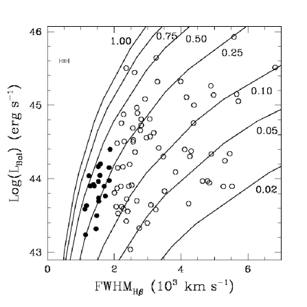
Figure 10.— Bolometric luminosities vs. FWHM_Hβ in the sample. Filled circles represent NLS1s, while open circles are broad line AGN, and the cross in the upper left corner gives the median uncertainty of the measurements. The curves track the expected locations of black holes with masses between $10^{4}M_{\odot}$ (bottom left side of the diagram) and $10^{9}M_{\odot}$ (upper right region) accreting at the labelled values of $\dot{M}/\dot{M}_{\rm Edd}$, if their emission were isotropic, the accretion efficiencies were $\eta=0.1$, and the BLR scaled as described in Bentz et al. (2006).

5. Discussion and conclusions

The main purpose of this work is to collect a large sample of flux and profile measurements of the broad emission line components in the Balmer series and to compare the results with those AGN properties that we were able to infer from the available data. The paper is intended as a starting point in a larger investigation aiming at the identifiaction of possible hints about the physical conditions within the BLR of many AGN, through the analysis of various broad lines.

While we spent a great effort in performing as carefully as possible our direct measurements on the broad emission lines, the size of our sample and the limited spectral coverage forced us to calculate the other source parameters by means of some simplified assumptions and empirical relations, which, in some cases, are still matter of debate. Using the BP method, we explored the relation of the temperature parameter $A$ and the broad line profiles. The values inferred in those objects where the technique achieved the best results would correspond to a temperature range running from $8\cdot 10^{3}\ {\rm K}$ to $21\cdot 10^{3}\ {\rm K}$, with cold gas being usually associated with broad line emitters. A better explanation of this result, which could be of fundamental importance in our understanding of the BLR structure, requires a deep investigation of the properties of the temperature parameter $A$ as a thermodynamic tool (ilic07). The possibility of a relation with the inferred accretion rates, too, deserves further investigation, since it may inform us about the different conditions of gas ionization or dust processing of the radiation within our point of view towards the BLR.

Taking into account the results of our measurements and the limits of the related assumptions, here we come to the following conclusions:

Figure 11.— Balmer line flux ratios of $H\delta$ (upper left panel), $H\gamma$ (upper right), and $H\alpha$ (lower left) together with the BP slope parameter (lower right panel) as a function of the Eddington ratio, with the same symbols as in Fig. 9. There appears to be a weak anti-correlation between the accretion rate and the Balmer decrement, with the high order lines being stronger in objects working at high Eddington ratios, resulting in modest BP slopes.

• the Balmer line flux ratios show a weak degree of correlation with the line profile width, in the sense that more pronounced Balmer decrements are observed in broader line emitting objects;

• the optical continuum luminosity of AGN is related to the emission line intensity of [O III], where we confirm the presence of a global Baldwin Effect, and of the broad components of the Balmer series, which, instead, do not show any strong evidence of global Baldwin Effect;

• the shape of the Balmer decrement, studied with the Boltzmann Plot technique, is related to the line profile widths and we observe that larger slopes and better straight line fits can be achieved in objects with broader lines, where a BLR component being described by the assumptions of this method may be present;

• we find a weak degree of anti-correlation between the Balmer decrement and the Eddington ratios measured in our sample, that could be the result of high dust column densities along our line of sight to the objects characterized by low accretion rates.

Table 1Line Flux and Boltzmann Plot analysis

Object Name	$F_{\rm H\beta}$	$R_{\rm H\epsilon}$	$R_{\rm H\delta}$	$R_{\rm H\gamma}$	$R_{\rm H\alpha}$	$F_{\rm[O\ III]}$	$A$	Class
SDSSJ0013–0951	427 $\pm$ 54	ND	0.24 $\pm$ 0.05	0.51 $\pm$ 0.08	3.89 $\pm$ 0.54	872 $\pm$ 63	0.302 $\pm$ 0.033	ii
SDSSJ0013+0052	1210 $\pm$ 108	ND	0.24 $\pm$ 0.04	0.42 $\pm$ 0.05	3.48 $\pm$ 0.33	237 $\pm$ 25	0.299 $\pm$ 0.011	ii
SDSSJ0037+0008	1054 $\pm$ 95	0.09 $\pm$ 0.02	0.21 $\pm$ 0.03	0.39 $\pm$ 0.06	3.39 $\pm$ 0.36	632 $\pm$ 65	0.344 $\pm$ 0.038	i
SDSSJ0042–1049	740 $\pm$ 87	ND	0.24 $\pm$ 0.05	0.49 $\pm$ 0.09	4.34 $\pm$ 0.56	637 $\pm$ 50	0.367 $\pm$ 0.032	ii
SDSSJ0107+1408	954 $\pm$ 72	0.10 $\pm$ 0.03	0.21 $\pm$ 0.04	0.45 $\pm$ 0.06	3.40 $\pm$ 0.30	242 $\pm$ 22	0.307 $\pm$ 0.023	i
SDSSJ0110–1008	5856 $\pm$ 452	0.10 $\pm$ 0.02	0.21 $\pm$ 0.03	0.43 $\pm$ 0.05	3.69 $\pm$ 0.31	3154 $\pm$ 126	0.349 $\pm$ 0.016	ii
SDSSJ0112+0003	702 $\pm$ 82	ND	0.28 $\pm$ 0.06	0.40 $\pm$ 0.08	4.04 $\pm$ 0.55	611 $\pm$ 16	0.353 $\pm$ 0.053	ii
SDSSJ0117+0000	956 $\pm$ 40	0.13 $\pm$ 0.04	0.27 $\pm$ 0.04	0.44 $\pm$ 0.03	3.22 $\pm$ 0.17	1194 $\pm$ 35	0.250 $\pm$ 0.015	i
SDSSJ0121–0102	1860 $\pm$ 137	ND	0.26 $\pm$ 0.04	0.40 $\pm$ 0.05	2.38 $\pm$ 0.23	334 $\pm$ 50	0.109 $\pm$ 0.049	iv
SDSSJ0135–0044	4053 $\pm$ 227	0.06 $\pm$ 0.01	0.20 $\pm$ 0.03	0.42 $\pm$ 0.04	3.40 $\pm$ 0.23	771 $\pm$ 60	0.339 $\pm$ 0.061	ii
SDSSJ0140–0050	1315 $\pm$ 100	ND	0.20 $\pm$ 0.05	0.41 $\pm$ 0.06	2.62 $\pm$ 0.25	473 $\pm$ 45	0.160 $\pm$ 0.044	iii
SDSSJ0142–1008	16431 $\pm$ 788	ND	0.22 $\pm$ 0.03	0.53 $\pm$ 0.06	3.89 $\pm$ 0.22	14866 $\pm$ 536	0.334 $\pm$ 0.048	ii
SDSSJ0142+0005	345 $\pm$ 37	ND	0.37 $\pm$ 0.09	0.65 $\pm$ 0.13	2.96 $\pm$ 0.37	233 $\pm$ 13	0.101 $\pm$ 0.071	iv
SDSSJ0150+1323	4297 $\pm$ 379	ND	0.18 $\pm$ 0.03	0.30 $\pm$ 0.05	4.18 $\pm$ 0.41	2272 $\pm$ 80	0.472 $\pm$ 0.041	ii
SDSSJ0159+0105	935 $\pm$ 100	ND	0.21 $\pm$ 0.05	0.41 $\pm$ 0.07	3.60 $\pm$ 0.42	296 $\pm$ 22	0.330 $\pm$ 0.008	ii
SDSSJ0233–0107	1067 $\pm$ 87	ND	0.20 $\pm$ 0.04	0.42 $\pm$ 0.05	3.63 $\pm$ 0.34	663 $\pm$ 33	0.340 $\pm$ 0.012	ii
SDSSJ0250+0025	940 $\pm$ 65	ND	0.32 $\pm$ 0.06	0.62 $\pm$ 0.08	3.62 $\pm$ 0.28	613 $\pm$ 37	0.229 $\pm$ 0.068	iii
SDSSJ0256+0113	964 $\pm$ 82	ND	0.21 $\pm$ 0.04	0.46 $\pm$ 0.06	3.54 $\pm$ 0.32	129 $\pm$ 21	0.301 $\pm$ 0.017	ii
SDSSJ0304+0028	618 $\pm$ 67	ND	0.27 $\pm$ 0.06	0.52 $\pm$ 0.09	2.11 $\pm$ 0.27	174 $\pm$ 24	0.002 $\pm$ 0.024	iv
SDSSJ0306+0003	496 $\pm$ 94	ND	0.38 $\pm$ 0.11	0.45 $\pm$ 0.11	3.14 $\pm$ 0.63	138 $\pm$ 8	0.167 $\pm$ 0.071	iv
SDSSJ0310–0049	1953 $\pm$ 113	ND	0.09 $\pm$ 0.02	0.29 $\pm$ 0.03	2.81 $\pm$ 0.21	293 $\pm$ 33	0.344 $\pm$ 0.137	iii
SDSSJ0322+0055	564 $\pm$ 68	ND	0.24 $\pm$ 0.05	0.48 $\pm$ 0.08	4.22 $\pm$ 0.56	408 $\pm$ 50	0.356 $\pm$ 0.031	ii
SDSSJ0323+0035	5994 $\pm$ 288	0.08 $\pm$ 0.01	0.21 $\pm$ 0.02	0.42 $\pm$ 0.04	3.19 $\pm$ 0.18	1729 $\pm$ 222	0.310 $\pm$ 0.046	i
SDSSJ0351–0526	7617 $\pm$ 454	0.12 $\pm$ 0.02	0.25 $\pm$ 0.03	0.47 $\pm$ 0.06	2.42 $\pm$ 0.18	6649 $\pm$ 310	0.124 $\pm$ 0.040	iv
SDSSJ0409–0429	4767 $\pm$ 310	ND	0.18 $\pm$ 0.03	0.37 $\pm$ 0.05	3.35 $\pm$ 0.26	1385 $\pm$ 42	0.339 $\pm$ 0.035	ii
SDSSJ0752+2617	487 $\pm$ 84	ND	0.33 $\pm$ 0.10	0.44 $\pm$ 0.12	2.61 $\pm$ 0.50	295 $\pm$ 24	0.110 $\pm$ 0.045	iv
SDSSJ0755+3911	2868 $\pm$ 290	0.14 $\pm$ 0.03	0.42 $\pm$ 0.07	0.53 $\pm$ 0.08	2.68 $\pm$ 0.30	1914 $\pm$ 63	0.058 $\pm$ 0.061	iv
SDSSJ0830+3405	4102 $\pm$ 265	ND	0.25 $\pm$ 0.04	0.46 $\pm$ 0.07	4.00 $\pm$ 0.29	1582 $\pm$ 92	0.350 $\pm$ 0.029	ii
SDSSJ0832+4614	2902 $\pm$ 217	0.10 $\pm$ 0.02	0.27 $\pm$ 0.04	0.42 $\pm$ 0.05	3.66 $\pm$ 0.30	1388 $\pm$ 54	0.314 $\pm$ 0.038	i
SDSSJ0839+4847	10536 $\pm$ 588	ND	0.21 $\pm$ 0.04	0.41 $\pm$ 0.05	3.65 $\pm$ 0.21	1164 $\pm$ 41	0.336 $\pm$ 0.002	ii
SDSSJ0840+0333	938 $\pm$ 73	ND	0.23 $\pm$ 0.04	0.46 $\pm$ 0.06	3.72 $\pm$ 0.32	439 $\pm$ 19	0.318 $\pm$ 0.018	ii
SDSSJ0855+5252	991 $\pm$ 122	ND	0.23 $\pm$ 0.05	0.49 $\pm$ 0.10	3.86 $\pm$ 0.51	430 $\pm$ 42	0.325 $\pm$ 0.032	ii
SDSSJ0857+0528	959 $\pm$ 127	ND	0.52 $\pm$ 0.13	0.77 $\pm$ 0.17	3.90 $\pm$ 0.55	1127 $\pm$ 52	0.146 $\pm$ 0.122	iv
SDSSJ0904+5536	699 $\pm$ 120	ND	0.24 $\pm$ 0.06	0.49 $\pm$ 0.12	3.55 $\pm$ 0.63	862 $\pm$ 24	0.273 $\pm$ 0.019	ii
SDSSJ0925+5335	406 $\pm$ 50	ND	0.64 $\pm$ 0.15	0.74 $\pm$ 0.14	3.22 $\pm$ 0.48	416 $\pm$ 22	0.008 $\pm$ 0.142	iv
SDSSJ0937+0105	1684 $\pm$ 92	ND	0.26 $\pm$ 0.04	0.55 $\pm$ 0.05	3.47 $\pm$ 0.22	1352 $\pm$ 76	0.230 $\pm$ 0.048	iii
SDSSJ1010+0043	2334 $\pm$ 139	0.11 $\pm$ 0.00	0.20 $\pm$ 0.02	0.45 $\pm$ 0.04	3.70 $\pm$ 0.28	1731 $\pm$ 64	0.351 $\pm$ 0.026	i
SDSSJ1013–0052	2300 $\pm$ 114	ND	0.15 $\pm$ 0.03	0.39 $\pm$ 0.05	1.56 $\pm$ 0.09	417 $\pm$ 54	-0.109 $\pm$ 0.117	iv
SDSSJ1016+4210	5835 $\pm$ 497	0.10 $\pm$ 0.02	0.36 $\pm$ 0.06	0.46 $\pm$ 0.07	2.56 $\pm$ 0.28	1497 $\pm$ 198	0.154 $\pm$ 0.096	iv
SDSSJ1025+5140	2045 $\pm$ 133	ND	0.30 $\pm$ 0.04	0.42 $\pm$ 0.05	3.64 $\pm$ 0.30	2349 $\pm$ 68	0.288 $\pm$ 0.057	iii
SDSSJ1042+0414	755 $\pm$ 71	ND	0.22 $\pm$ 0.05	0.61 $\pm$ 0.09	3.75 $\pm$ 0.40	1037 $\pm$ 66	0.266 $\pm$ 0.076	iii
SDSSJ1057–0041	1087 $\pm$ 76	ND	0.37 $\pm$ 0.07	0.57 $\pm$ 0.04	2.76 $\pm$ 0.23	357 $\pm$ 29	0.078 $\pm$ 0.035	iv
SDSSJ1059–0005	934 $\pm$ 86	ND	0.22 $\pm$ 0.04	0.46 $\pm$ 0.09	2.26 $\pm$ 0.23	162 $\pm$ 32	0.087 $\pm$ 0.046	iv
SDSSJ1105+0745	1610 $\pm$ 186	ND	0.22 $\pm$ 0.06	0.35 $\pm$ 0.06	3.80 $\pm$ 0.47	589 $\pm$ 25	0.392 $\pm$ 0.032	ii
SDSSJ1118+5803	10103 $\pm$ 594	ND	0.27 $\pm$ 0.04	0.48 $\pm$ 0.06	4.12 $\pm$ 0.28	7199 $\pm$ 279	0.350 $\pm$ 0.047	ii
SDSSJ1122+0117	1791 $\pm$ 115	ND	0.22 $\pm$ 0.04	0.45 $\pm$ 0.06	3.68 $\pm$ 0.32	2470 $\pm$ 69	0.327 $\pm$ 0.017	ii
SDSSJ1128+1023	2622 $\pm$ 262	ND	0.32 $\pm$ 0.08	0.52 $\pm$ 0.08	3.92 $\pm$ 0.45	2644 $\pm$ 208	0.284 $\pm$ 0.059	iii
SDSSJ1139+5911	1654 $\pm$ 160	0.16 $\pm$ 0.05	0.28 $\pm$ 0.06	0.59 $\pm$ 0.09	2.56 $\pm$ 0.31	887 $\pm$ 52	0.072 $\pm$ 0.031	iv
SDSSJ1141+0241	1109 $\pm$ 285	ND	0.28 $\pm$ 0.11	0.58 $\pm$ 0.18	3.03 $\pm$ 0.80	377 $\pm$ 13	0.130 $\pm$ 0.031	iv
SDSSJ1152–0005	859 $\pm$ 79	0.20 $\pm$ 0.06	0.25 $\pm$ 0.05	0.44 $\pm$ 0.08	2.02 $\pm$ 0.20	332 $\pm$ 48	0.003 $\pm$ 0.031	iv
SDSSJ1157–0022	5477 $\pm$ 177	ND	0.11 $\pm$ 0.02	0.32 $\pm$ 0.04	2.96 $\pm$ 0.13	990 $\pm$ 48	0.260 $\pm$ 0.084	iv
SDSSJ1157+0412	2188 $\pm$ 195	0.13 $\pm$ 0.02	0.27 $\pm$ 0.06	0.44 $\pm$ 0.08	3.36 $\pm$ 0.31	739 $\pm$ 111	0.268 $\pm$ 0.014	i
SDSSJ1203+0229	3719 $\pm$ 270	0.12 $\pm$ 0.02	0.20 $\pm$ 0.03	0.42 $\pm$ 0.04	3.17 $\pm$ 0.24	501 $\pm$ 80	0.282 $\pm$ 0.016	i
SDSSJ1223+0240	870 $\pm$ 97	ND	0.25 $\pm$ 0.06	0.55 $\pm$ 0.09	3.66 $\pm$ 0.43	987 $\pm$ 40	0.266 $\pm$ 0.039	ii
SDSSJ1243+0252	738 $\pm$ 51	ND	0.20 $\pm$ 0.03	0.45 $\pm$ 0.06	3.49 $\pm$ 0.28	132 $\pm$ 24	0.316 $\pm$ 0.023	ii
SDSSJ1246+0222	3619 $\pm$ 160	ND	0.29 $\pm$ 0.03	0.52 $\pm$ 0.04	3.29 $\pm$ 0.17	1982 $\pm$ 73	0.216 $\pm$ 0.036	iii
SDSSJ1300+5641	1731 $\pm$ 146	ND	0.25 $\pm$ 0.06	0.45 $\pm$ 0.06	3.59 $\pm$ 0.32	1088 $\pm$ 43	0.280 $\pm$ 0.019	ii
SDSSJ1300+6139	2488 $\pm$ 128	ND	0.30 $\pm$ 0.05	0.50 $\pm$ 0.06	3.93 $\pm$ 0.27	1105 $\pm$ 54	0.328 $\pm$ 0.061	ii
SDSSJ1307–0036	1204 $\pm$ 80	0.08 $\pm$ 0.02	0.22 $\pm$ 0.03	0.41 $\pm$ 0.05	2.79 $\pm$ 0.20	537 $\pm$ 35	0.207 $\pm$ 0.039	iii
SDSSJ1307+0107	1956 $\pm$ 109	0.06 $\pm$ 0.01	0.23 $\pm$ 0.04	0.40 $\pm$ 0.04	4.51 $\pm$ 0.40	1389 $\pm$ 56	0.476 $\pm$ 0.075	i
SDSSJ1331+0131	2753 $\pm$ 268	0.17 $\pm$ 0.03	0.39 $\pm$ 0.08	0.40 $\pm$ 0.06	2.40 $\pm$ 0.26	2120 $\pm$ 269	0.074 $\pm$ 0.059	iv
SDSSJ1341–0053	1433 $\pm$ 99	0.11 $\pm$ 0.02	0.23 $\pm$ 0.03	0.39 $\pm$ 0.05	3.46 $\pm$ 0.30	1174 $\pm$ 42	0.320 $\pm$ 0.020	i
SDSSJ1342–0053	840 $\pm$ 90	ND	0.27 $\pm$ 0.05	0.49 $\pm$ 0.07	4.00 $\pm$ 0.47	355 $\pm$ 25	0.309 $\pm$ 0.038	ii
SDSSJ1342+5642	903 $\pm$ 78	ND	0.20 $\pm$ 0.05	0.48 $\pm$ 0.08	3.47 $\pm$ 0.34	155 $\pm$ 13	0.291 $\pm$ 0.030	ii
SDSSJ1343+0004	1269 $\pm$ 122	0.14 $\pm$ 0.03	0.34 $\pm$ 0.06	0.52 $\pm$ 0.07	3.23 $\pm$ 0.36	462 $\pm$ 53	0.188 $\pm$ 0.043	iii
SDSSJ1344–0015	1577 $\pm$ 136	0.14 $\pm$ 0.03	0.34 $\pm$ 0.05	0.49 $\pm$ 0.05	2.48 $\pm$ 0.84	406 $\pm$ 117	0.065 $\pm$ 0.109	iv
SDSSJ1344+0005	1912 $\pm$ 103	ND	0.11 $\pm$ 0.02	0.32 $\pm$ 0.04	3.53 $\pm$ 0.22	428 $\pm$ 31	0.397 $\pm$ 0.073	iii
SDSSJ1344+4416	2292 $\pm$ 238	ND	0.39 $\pm$ 0.08	0.42 $\pm$ 0.08	2.11 $\pm$ 0.24	512 $\pm$ 81	-0.017 $\pm$ 0.062	iv
SDSSJ1345–0259	3518 $\pm$ 243	ND	0.31 $\pm$ 0.04	0.47 $\pm$ 0.05	2.94 $\pm$ 0.23	1317 $\pm$ 46	0.154 $\pm$ 0.033	iii
SDSSJ1349+0204	3930 $\pm$ 220	ND	0.22 $\pm$ 0.03	0.41 $\pm$ 0.06	4.87 $\pm$ 0.30	8162 $\pm$ 260	0.496 $\pm$ 0.030	ii
SDSSJ1355+6440	4383 $\pm$ 352	0.13 $\pm$ 0.02	0.32 $\pm$ 0.05	0.47 $\pm$ 0.06	2.65 $\pm$ 0.23	2483 $\pm$ 163	0.136 $\pm$ 0.033	iii
SDSSJ1437+0007	1321 $\pm$ 87	0.12 $\pm$ 0.02	0.22 $\pm$ 0.02	0.50 $\pm$ 0.06	3.07 $\pm$ 0.25	335 $\pm$ 43	0.251 $\pm$ 0.029	i
SDSSJ1505+0342	1348 $\pm$ 144	0.14 $\pm$ 0.04	0.43 $\pm$ 0.08	0.58 $\pm$ 0.10	3.27 $\pm$ 0.38	1202 $\pm$ 29	0.140 $\pm$ 0.066	iv

Table 1Line Flux and Boltzmann Plot analysis

Object Name	$F_{\rm H\beta}$	$R_{\rm H\epsilon}$	$R_{\rm H\delta}$	$R_{\rm H\gamma}$	$R_{\rm H\alpha}$	$F_{\rm[O\ III]}$	$A$	Class
SDSSJ1510+0058	10659 $\pm$ 695	ND	0.23 $\pm$ 0.03	0.38 $\pm$ 0.04	4.00 $\pm$ 0.31	15250 $\pm$ 377	0.392 $\pm$ 0.027	ii
SDSSJ1519+0016	1306 $\pm$ 133	ND	0.25 $\pm$ 0.06	0.43 $\pm$ 0.05	3.61 $\pm$ 0.45	392 $\pm$ 27	0.316 $\pm$ 0.013	ii
SDSSJ1519+5908	1596 $\pm$ 131	0.13 $\pm$ 0.03	0.32 $\pm$ 0.07	0.50 $\pm$ 0.07	2.94 $\pm$ 0.26	416 $\pm$ 72	0.179 $\pm$ 0.034	iii
SDSSJ1535+5754	1658 $\pm$ 122	ND	0.23 $\pm$ 0.04	0.39 $\pm$ 0.05	3.45 $\pm$ 0.28	238 $\pm$ 25	0.304 $\pm$ 0.018	ii
SDSSJ1538+4440	1212 $\pm$ 90	ND	0.28 $\pm$ 0.05	0.45 $\pm$ 0.07	2.96 $\pm$ 0.25	1017 $\pm$ 30	0.185 $\pm$ 0.020	iii
SDSSJ1554+3238	3053 $\pm$ 283	ND	0.29 $\pm$ 0.06	0.40 $\pm$ 0.07	4.78 $\pm$ 0.46	3065 $\pm$ 116	0.440 $\pm$ 0.061	ii
SDSSJ1613+3717	1797 $\pm$ 193	ND	0.24 $\pm$ 0.05	0.42 $\pm$ 0.06	4.12 $\pm$ 0.48	528 $\pm$ 17	0.387 $\pm$ 0.022	ii
SDSSJ1619+4058	2609 $\pm$ 164	ND	0.30 $\pm$ 0.05	0.52 $\pm$ 0.08	4.40 $\pm$ 0.31	6830 $\pm$ 293	0.374 $\pm$ 0.070	ii
SDSSJ1623+4104	6033 $\pm$ 481	0.09 $\pm$ 0.02	0.28 $\pm$ 0.05	0.40 $\pm$ 0.06	2.31 $\pm$ 0.20	1254 $\pm$ 186	0.114 $\pm$ 0.056	iv
SDSSJ1654+3925	2396 $\pm$ 178	ND	0.28 $\pm$ 0.07	0.47 $\pm$ 0.07	3.88 $\pm$ 0.32	3564 $\pm$ 131	0.334 $\pm$ 0.037	ii
SDSSJ1659+6202	1440 $\pm$ 101	ND	0.25 $\pm$ 0.04	0.41 $\pm$ 0.05	3.10 $\pm$ 0.24	149 $\pm$ 27	0.251 $\pm$ 0.019	ii
SDSSJ1717+5815	1906 $\pm$ 144	ND	0.20 $\pm$ 0.04	0.40 $\pm$ 0.07	2.27 $\pm$ 0.22	521 $\pm$ 49	0.096 $\pm$ 0.065	iv
SDSSJ1719+5937	5646 $\pm$ 297	ND	0.13 $\pm$ 0.02	0.37 $\pm$ 0.04	4.36 $\pm$ 0.34	1955 $\pm$ 144	0.525 $\pm$ 0.072	ii
SDSSJ1720+5540	3722 $\pm$ 253	ND	0.24 $\pm$ 0.04	0.40 $\pm$ 0.04	3.54 $\pm$ 0.26	5491 $\pm$ 213	0.323 $\pm$ 0.016	ii
SDSSJ2058–0650	1116 $\pm$ 191	ND	0.20 $\pm$ 0.06	0.39 $\pm$ 0.10	2.57 $\pm$ 0.48	296 $\pm$ 30	0.204 $\pm$ 0.036	iii
SDSSJ2349–0036	1837 $\pm$ 176	ND	0.34 $\pm$ 0.06	0.54 $\pm$ 0.08	3.05 $\pm$ 0.33	519 $\pm$ 45	0.146 $\pm$ 0.043	iv
SDSSJ2351–0109	522 $\pm$ 52	ND	0.26 $\pm$ 0.04	0.47 $\pm$ 0.09	3.06 $\pm$ 0.35	186 $\pm$ 17	0.201 $\pm$ 0.013	iii

Table 2Line profile and source property estimates

Object Name	FWHM	FWZI	$L_{5100}$	$R_{\rm BLR}$	$M_{\rm BH}$	$\dot{M}/\dot{M}_{\rm Edd}$
SDSSJ0013–0951	1122 $\pm$ 150	5951 $\pm$ 1632	3.86 $\pm$ 0.17	11.35 $\pm$ 1.31	8.08 $\pm$ 0.93	0.405 $\pm$ 0.064
SDSSJ0013+0052	4163 $\pm$ 234	10573 $\pm$ 1458	128.04 $\pm$ 1.06	65.35 $\pm$ 6.43	639.96 $\pm$ 62.92	0.170 $\pm$ 0.018
SDSSJ0037+0008	2608 $\pm$ 150	8744 $\pm$ 1467	277.83 $\pm$ 4.94	96.27 $\pm$ 9.92	369.99 $\pm$ 38.13	0.636 $\pm$ 0.077
SDSSJ0042–1049	2272 $\pm$ 150	7478 $\pm$ 1355	3.89 $\pm$ 0.08	11.40 $\pm$ 1.19	33.23 $\pm$ 3.46	0.099 $\pm$ 0.012
SDSSJ0107+1408	2214 $\pm$ 150	8956 $\pm$ 1661	56.76 $\pm$ 1.39	43.51 $\pm$ 4.63	120.52 $\pm$ 12.83	0.399 $\pm$ 0.052
SDSSJ0110–1008	2808 $\pm$ 216	10537 $\pm$ 1261	53.19 $\pm$ 0.46	42.12 $\pm$ 4.15	187.64 $\pm$ 18.49	0.240 $\pm$ 0.026
SDSSJ0112+0003	2218 $\pm$ 179	8524 $\pm$ 2044	4.16 $\pm$ 0.05	11.78 $\pm$ 1.19	32.75 $\pm$ 3.29	0.108 $\pm$ 0.012
SDSSJ0117+0000	2571 $\pm$ 243	8610 $\pm$ 1831	33.58 $\pm$ 1.53	33.47 $\pm$ 3.91	124.96 $\pm$ 14.61	0.228 $\pm$ 0.037
SDSSJ0121–0102	3253 $\pm$ 150	9969 $\pm$ 1480	439.86 $\pm$ 2.73	121.13 $\pm$ 11.78	724.50 $\pm$ 70.48	0.515 $\pm$ 0.053
SDSSJ0135–0044	5586 $\pm$ 379	12992 $\pm$ 1813	845.06 $\pm$ 14.18	167.90 $\pm$ 17.22	2960.01 $\pm$ 303.58	0.242 $\pm$ 0.029
SDSSJ0140–0050	2621 $\pm$ 150	9068 $\pm$ 1374	22.95 $\pm$ 0.33	27.67 $\pm$ 2.80	107.38 $\pm$ 10.88	0.181 $\pm$ 0.021
SDSSJ0142–1008	4266 $\pm$ 150	12344 $\pm$ 2467	20.11 $\pm$ 0.31	25.90 $\pm$ 2.64	266.31 $\pm$ 27.10	0.064 $\pm$ 0.007
SDSSJ0142+0005	1142 $\pm$ 150	5568 $\pm$ 1203	1.73 $\pm$ 0.08	7.59 $\pm$ 0.88	5.59 $\pm$ 0.65	0.262 $\pm$ 0.042
SDSSJ0150+1323	4846 $\pm$ 410	14046 $\pm$ 3127	8.78 $\pm$ 0.13	17.12 $\pm$ 1.73	227.13 $\pm$ 23.01	0.033 $\pm$ 0.004
SDSSJ0159+0105	3077 $\pm$ 201	9978 $\pm$ 2151	37.36 $\pm$ 0.65	35.30 $\pm$ 3.63	188.85 $\pm$ 19.42	0.168 $\pm$ 0.020
SDSSJ0233–0107	3330 $\pm$ 291	9277 $\pm$ 1278	26.13 $\pm$ 0.50	29.52 $\pm$ 3.07	184.98 $\pm$ 19.20	0.120 $\pm$ 0.015
SDSSJ0250+0025	1453 $\pm$ 150	6686 $\pm$ 1400	2.07 $\pm$ 0.07	8.32 $\pm$ 0.91	9.93 $\pm$ 1.09	0.177 $\pm$ 0.025
SDSSJ0256+0113	3504 $\pm$ 150	8969 $\pm$ 1945	6.76 $\pm$ 0.18	15.01 $\pm$ 1.61	104.17 $\pm$ 11.19	0.055 $\pm$ 0.007
SDSSJ0304+0028	2922 $\pm$ 157	8149 $\pm$ 1091	120.96 $\pm$ 1.85	63.52 $\pm$ 6.47	306.39 $\pm$ 31.19	0.335 $\pm$ 0.039
SDSSJ0306+0003	1474 $\pm$ 185	7004 $\pm$ 1460	3.14 $\pm$ 0.13	10.23 $\pm$ 1.18	12.56 $\pm$ 1.44	0.212 $\pm$ 0.033
SDSSJ0310–0049	4372 $\pm$ 150	10846 $\pm$ 1882	57.01 $\pm$ 1.14	43.61 $\pm$ 4.54	471.05 $\pm$ 49.07	0.103 $\pm$ 0.013
SDSSJ0322+0055	2005 $\pm$ 150	6805 $\pm$ 1110	6.44 $\pm$ 0.22	14.66 $\pm$ 1.64	33.31 $\pm$ 3.72	0.164 $\pm$ 0.024
SDSSJ0323+0035	2356 $\pm$ 150	9902 $\pm$ 1747	318.83 $\pm$ 2.38	103.13 $\pm$ 10.10	323.42 $\pm$ 31.66	0.835 $\pm$ 0.088
SDSSJ0351–0526	2563 $\pm$ 162	8176 $\pm$ 1738	31.62 $\pm$ 0.72	32.48 $\pm$ 3.43	120.58 $\pm$ 12.73	0.222 $\pm$ 0.029
SDSSJ0409–0429	3181 $\pm$ 154	9837 $\pm$ 1301	41.92 $\pm$ 0.42	37.40 $\pm$ 3.71	213.82 $\pm$ 21.21	0.166 $\pm$ 0.018
SDSSJ0752+2617	2009 $\pm$ 150	7978 $\pm$ 1915	6.39 $\pm$ 0.17	14.60 $\pm$ 1.57	33.30 $\pm$ 3.58	0.163 $\pm$ 0.022
SDSSJ0755+3911	1697 $\pm$ 150	7686 $\pm$ 1003	7.88 $\pm$ 0.09	16.21 $\pm$ 1.62	26.39 $\pm$ 2.63	0.253 $\pm$ 0.028
SDSSJ0830+3405	5460 $\pm$ 239	13492 $\pm$ 1879	21.87 $\pm$ 0.55	27.01 $\pm$ 2.89	454.94 $\pm$ 48.60	0.041 $\pm$ 0.005
SDSSJ0832+4614	2199 $\pm$ 176	10423 $\pm$ 1518	7.87 $\pm$ 0.16	16.21 $\pm$ 1.69	44.30 $\pm$ 4.62	0.151 $\pm$ 0.019
SDSSJ0839+4847	5526 $\pm$ 179	14898 $\pm$ 3208	7.86 $\pm$ 0.13	16.19 $\pm$ 1.66	279.34 $\pm$ 28.70	0.024 $\pm$ 0.003
SDSSJ0840+0333	4227 $\pm$ 234	9804 $\pm$ 1742	4.57 $\pm$ 0.06	12.35 $\pm$ 1.24	124.70 $\pm$ 12.51	0.031 $\pm$ 0.003
SDSSJ0855+5252	1736 $\pm$ 150	6162 $\pm$ 1113	5.81 $\pm$ 0.23	13.92 $\pm$ 1.58	23.72 $\pm$ 2.69	0.208 $\pm$ 0.032
SDSSJ0857+0528	2359 $\pm$ 150	7423 $\pm$ 1429	2.64 $\pm$ 0.02	9.39 $\pm$ 0.93	29.51 $\pm$ 2.91	0.076 $\pm$ 0.008
SDSSJ0904+5536	2483 $\pm$ 163	6940 $\pm$ 1361	1.09 $\pm$ 0.01	6.02 $\pm$ 0.60	20.98 $\pm$ 2.10	0.044 $\pm$ 0.005
SDSSJ0925+5335	1532 $\pm$ 150	5811 $\pm$ 1291	5.44 $\pm$ 0.07	13.47 $\pm$ 1.35	17.86 $\pm$ 1.79	0.258 $\pm$ 0.029
SDSSJ0937+0105	2258 $\pm$ 150	7719 $\pm$ 1285	14.45 $\pm$ 0.53	21.95 $\pm$ 2.47	63.25 $\pm$ 7.12	0.194 $\pm$ 0.029
SDSSJ1010+0043	2806 $\pm$ 150	8138 $\pm$ 1723	64.08 $\pm$ 2.98	46.23 $\pm$ 5.43	205.76 $\pm$ 24.16	0.264 $\pm$ 0.043
SDSSJ1013–0052	6816 $\pm$ 164	11309 $\pm$ 1542	324.69 $\pm$ 3.59	104.07 $\pm$ 10.38	2732.11 $\pm$ 272.37	0.101 $\pm$ 0.011
SDSSJ1016+4210	1845 $\pm$ 150	9904 $\pm$ 2052	14.11 $\pm$ 0.43	21.70 $\pm$ 2.37	41.73 $\pm$ 4.56	0.287 $\pm$ 0.040
SDSSJ1025+5140	1845 $\pm$ 226	9883 $\pm$ 1104	9.42 $\pm$ 0.08	17.73 $\pm$ 1.75	34.11 $\pm$ 3.36	0.234 $\pm$ 0.025
SDSSJ1042+0414	2082 $\pm$ 150	7751 $\pm$ 1499	7.41 $\pm$ 0.17	15.72 $\pm$ 1.67	38.49 $\pm$ 4.08	0.163 $\pm$ 0.021
SDSSJ1057–0041	2370 $\pm$ 150	8870 $\pm$ 2027	5.28 $\pm$ 0.13	13.27 $\pm$ 1.41	42.13 $\pm$ 4.47	0.106 $\pm$ 0.014
SDSSJ1059–0005	2674 $\pm$ 174	9662 $\pm$ 1278	92.33 $\pm$ 1.12	55.50 $\pm$ 5.56	224.16 $\pm$ 22.47	0.349 $\pm$ 0.039
SDSSJ1105+0745	5268 $\pm$ 262	15224 $\pm$ 2513	7.83 $\pm$ 0.18	16.16 $\pm$ 1.71	253.36 $\pm$ 26.83	0.026 $\pm$ 0.003
SDSSJ1118+5803	4107 $\pm$ 150	12589 $\pm$ 2159	25.00 $\pm$ 0.74	28.88 $\pm$ 3.15	275.20 $\pm$ 29.99	0.077 $\pm$ 0.011
SDSSJ1122+0117	1534 $\pm$ 164	7596 $\pm$ 1698	4.94 $\pm$ 0.08	12.84 $\pm$ 1.31	17.08 $\pm$ 1.75	0.245 $\pm$ 0.029
SDSSJ1128+1023	1244 $\pm$ 150	6968 $\pm$ 1366	10.94 $\pm$ 0.28	19.11 $\pm$ 2.04	16.71 $\pm$ 1.79	0.555 $\pm$ 0.073
SDSSJ1139+5911	2459 $\pm$ 150	8101 $\pm$ 1995	15.60 $\pm$ 0.14	22.81 $\pm$ 2.25	77.92 $\pm$ 7.67	0.170 $\pm$ 0.018
SDSSJ1141+0241	2114 $\pm$ 263	8755 $\pm$ 2906	3.37 $\pm$ 0.03	10.60 $\pm$ 1.04	26.76 $\pm$ 2.63	0.107 $\pm$ 0.011
SDSSJ1152–0005	2693 $\pm$ 150	7488 $\pm$ 1375	77.88 $\pm$ 2.72	50.97 $\pm$ 5.69	208.85 $\pm$ 23.31	0.316 $\pm$ 0.046
SDSSJ1157–0022	5662 $\pm$ 214	13711 $\pm$ 2510	140.86 $\pm$ 3.26	68.55 $\pm$ 7.25	1241.78 $\pm$ 131.30	0.096 $\pm$ 0.012
SDSSJ1157+0412	1522 $\pm$ 150	7755 $\pm$ 1910	14.61 $\pm$ 0.67	22.07 $\pm$ 2.59	28.90 $\pm$ 3.38	0.428 $\pm$ 0.070
SDSSJ1203+0229	2963 $\pm$ 150	10524 $\pm$ 1714	35.99 $\pm$ 0.24	34.65 $\pm$ 3.38	171.89 $\pm$ 16.76	0.177 $\pm$ 0.018
SDSSJ1223+0240	2521 $\pm$ 150	7832 $\pm$ 1657	8.15 $\pm$ 0.11	16.48 $\pm$ 1.66	59.21 $\pm$ 5.96	0.117 $\pm$ 0.013
SDSSJ1243+0252	1168 $\pm$ 150	5511 $\pm$ 1239	4.31 $\pm$ 0.23	11.99 $\pm$ 1.45	9.24 $\pm$ 1.12	0.395 $\pm$ 0.069
SDSSJ1246+0222	2782 $\pm$ 159	9034 $\pm$ 1683	45.44 $\pm$ 0.32	38.93 $\pm$ 3.80	170.30 $\pm$ 16.63	0.226 $\pm$ 0.024
SDSSJ1300+5641	2104 $\pm$ 170	9338 $\pm$ 1766	13.98 $\pm$ 0.21	21.60 $\pm$ 2.19	54.01 $\pm$ 5.49	0.219 $\pm$ 0.026
SDSSJ1300+6139	4644 $\pm$ 239	11765 $\pm$ 1589	9.25 $\pm$ 0.10	17.57 $\pm$ 1.75	214.11 $\pm$ 21.31	0.037 $\pm$ 0.004
SDSSJ1307–0036	2556 $\pm$ 150	9077 $\pm$ 1663	48.84 $\pm$ 0.53	40.36 $\pm$ 4.02	149.05 $\pm$ 14.85	0.278 $\pm$ 0.031
SDSSJ1307+0107	4890 $\pm$ 231	15868 $\pm$ 2613	183.28 $\pm$ 2.67	78.19 $\pm$ 7.93	1056.59 $\pm$ 107.19	0.147 $\pm$ 0.017
SDSSJ1331+0131	1569 $\pm$ 150	7615 $\pm$ 1448	11.05 $\pm$ 0.44	19.20 $\pm$ 2.19	26.69 $\pm$ 3.05	0.351 $\pm$ 0.054
SDSSJ1341–0053	2300 $\pm$ 150	8993 $\pm$ 1537	32.02 $\pm$ 0.64	32.68 $\pm$ 3.40	97.72 $\pm$ 10.18	0.278 $\pm$ 0.034
SDSSJ1342–0053	4301 $\pm$ 150	10310 $\pm$ 1888	23.61 $\pm$ 0.14	28.06 $\pm$ 2.72	293.32 $\pm$ 28.47	0.068 $\pm$ 0.007
SDSSJ1342+5642	2676 $\pm$ 150	8311 $\pm$ 1699	4.99 $\pm$ 0.07	12.90 $\pm$ 1.31	52.18 $\pm$ 5.31	0.081 $\pm$ 0.009
SDSSJ1343+0004	1873 $\pm$ 150	7648 $\pm$ 2218	25.02 $\pm$ 0.42	28.89 $\pm$ 2.96	57.24 $\pm$ 5.87	0.370 $\pm$ 0.044
SDSSJ1344–0015	2086 $\pm$ 150	8591 $\pm$ 2372	30.36 $\pm$ 0.42	31.82 $\pm$ 3.22	78.27 $\pm$ 7.92	0.329 $\pm$ 0.038
SDSSJ1344+0005	5717 $\pm$ 150	14506 $\pm$ 2272	113.00 $\pm$ 2.11	61.40 $\pm$ 6.35	1133.83 $\pm$ 117.35	0.084 $\pm$ 0.010
SDSSJ1344+4416	1372 $\pm$ 150	8145 $\pm$ 2017	8.30 $\pm$ 0.18	16.63 $\pm$ 1.75	17.68 $\pm$ 1.86	0.398 $\pm$ 0.051
SDSSJ1345–0259	3097 $\pm$ 205	11282 $\pm$ 1869	4.39 $\pm$ 0.03	12.10 $\pm$ 1.18	65.57 $\pm$ 6.40	0.057 $\pm$ 0.006
SDSSJ1349+0204	2990 $\pm$ 681	9396 $\pm$ 1882	2.48 $\pm$ 0.11	9.10 $\pm$ 1.05	45.98 $\pm$ 5.32	0.046 $\pm$ 0.007
SDSSJ1355+6440	1527 $\pm$ 150	7214 $\pm$ 1614	9.14 $\pm$ 0.34	17.46 $\pm$ 1.96	23.00 $\pm$ 2.59	0.337 $\pm$ 0.050
SDSSJ1437+0007	2278 $\pm$ 151	8801 $\pm$ 2287	74.76 $\pm$ 0.79	49.94 $\pm$ 4.97	146.48 $\pm$ 14.57	0.433 $\pm$ 0.048
SDSSJ1505+0342	1400 $\pm$ 150	7570 $\pm$ 1644	7.98 $\pm$ 0.12	16.32 $\pm$ 1.66	18.08 $\pm$ 1.84	0.374 $\pm$ 0.044

Table 2Line profile and source property estimates

Object Name	FWHM	FWZI	$L_{5100}$	$R_{\rm BLR}$	$M_{\rm BH}$	$\dot{M}/\dot{M}_{\rm Edd}$
SDSSJ1510+0058	4906 $\pm$ 266	11785 $\pm$ 2483	21.63 $\pm$ 0.35	26.86 $\pm$ 2.75	365.27 $\pm$ 37.34	0.050 $\pm$ 0.006
SDSSJ1519+0016	4387 $\pm$ 171	10600 $\pm$ 1802	100.02 $\pm$ 1.65	57.76 $\pm$ 5.92	628.19 $\pm$ 64.34	0.135 $\pm$ 0.016
SDSSJ1519+5908	1278 $\pm$ 150	6936 $\pm$ 1521	7.95 $\pm$ 0.30	16.29 $\pm$ 1.84	15.03 $\pm$ 1.70	0.448 $\pm$ 0.067
SDSSJ1535+5754	3834 $\pm$ 322	10655 $\pm$ 1295	12.30 $\pm$ 0.09	20.26 $\pm$ 1.98	168.21 $\pm$ 16.43	0.062 $\pm$ 0.006
SDSSJ1538+4440	3242 $\pm$ 188	8706 $\pm$ 1439	3.79 $\pm$ 0.03	11.24 $\pm$ 1.11	66.77 $\pm$ 6.59	0.048 $\pm$ 0.005
SDSSJ1554+3238	5312 $\pm$ 382	10818 $\pm$ 1375	17.46 $\pm$ 0.29	24.14 $\pm$ 2.47	384.87 $\pm$ 39.40	0.038 $\pm$ 0.005
SDSSJ1613+3717	4789 $\pm$ 217	11267 $\pm$ 1272	9.27 $\pm$ 0.10	17.58 $\pm$ 1.75	227.90 $\pm$ 22.64	0.034 $\pm$ 0.004
SDSSJ1619+4058	2436 $\pm$ 150	8016 $\pm$ 2087	7.88 $\pm$ 0.17	16.21 $\pm$ 1.70	54.35 $\pm$ 5.71	0.123 $\pm$ 0.016
SDSSJ1623+4104	1586 $\pm$ 150	8242 $\pm$ 1964	15.86 $\pm$ 0.37	23.00 $\pm$ 2.43	32.67 $\pm$ 3.45	0.411 $\pm$ 0.053
SDSSJ1654+3925	2402 $\pm$ 207	7030 $\pm$ 1450	3.60 $\pm$ 0.09	10.96 $\pm$ 1.17	35.71 $\pm$ 3.81	0.085 $\pm$ 0.011
SDSSJ1659+6202	3990 $\pm$ 150	9829 $\pm$ 1132	210.04 $\pm$ 2.34	83.71 $\pm$ 8.35	752.96 $\pm$ 75.10	0.236 $\pm$ 0.026
SDSSJ1717+5815	3292 $\pm$ 159	9966 $\pm$ 1622	208.76 $\pm$ 2.27	83.45 $\pm$ 8.31	511.13 $\pm$ 50.91	0.346 $\pm$ 0.038
SDSSJ1719+5937	4973 $\pm$ 216	20280 $\pm$ 3400	137.49 $\pm$ 5.19	67.72 $\pm$ 7.66	946.25 $\pm$ 106.97	0.123 $\pm$ 0.019
SDSSJ1720+5540	3469 $\pm$ 244	10064 $\pm$ 1750	19.96 $\pm$ 0.20	25.80 $\pm$ 2.56	175.40 $\pm$ 17.40	0.096 $\pm$ 0.011
SDSSJ2058–0650	2058 $\pm$ 150	8580 $\pm$ 1663	4.15 $\pm$ 0.10	11.77 $\pm$ 1.25	28.15 $\pm$ 2.99	0.125 $\pm$ 0.016
SDSSJ2349–0036	2749 $\pm$ 150	8662 $\pm$ 1328	2.13 $\pm$ 0.10	8.43 $\pm$ 0.99	35.98 $\pm$ 4.21	0.050 $\pm$ 0.008
SDSSJ2351–0109	3062 $\pm$ 153	9042 $\pm$ 1614	64.75 $\pm$ 0.43	46.47 $\pm$ 4.53	246.21 $\pm$ 24.00	0.223 $\pm$ 0.023

References

- Baldwin (1977) Baldwin, J. A. 1977, ApJ, 214, 679
- Bentz et al. (2006) Bentz, M. C., Peterson, B. M., Pogge, R. W., Vestergaard, M., Onken, C. A. 2006, ApJ, 644, 133
- Bian (2005) Bian, W.-H. 2005, CJAA, 5, 21
- Binette, Fosbury, & Parker (1993) Binette, L., Fosbury, R. A., Parker, D. 1993, PASP, 105, 1150
- Boller, Brandt, & Fink (1996) Boller, T., Brandt, W. N., Fink, H. 1996, A&A, 305, 53
- Bon et al. (2006) Bon, E., Popović, L. Č., Ilić, D., Mediavilla, E. 2006, NewAR, 50, 716
- Boroson (2003) Boroson, T. A. 2003, ApJ, 585, 647
- Botte et al. (2004) Botte, V., Ciroi, S., Rafanelli, P., Di Mille, F. 2004, AJ, 127, 3168
- Cardelli, Clayton, & Mathis (1989) Cardelli, J. A., Clayton, G. C., Mathis, J. S. 1989, ApJ, 345, 245
- Connolly et al. (1995) Connolly, A. J., Szalay, A. S., Bershady, M. A., Kinney, A. L., & Calzetti, D. 1995, AJ, 110, 1071
- Gilbert & Peterson (2003) Gilbert, K. M., Peterson, B. M. 2003, ApJ, 587, 123
- Goad, Korista, & Knigge (2004) Goad, M. R., Korista, K. T., & Knigge, C. 2004, MNRAS, 325, 277
- Ilić et al. (2006) Ilić, D., Popović, L. Č., Bon, E., Mediavilla, E. G., Chavushyan, V. H. 2006, MNRAS, 371, 1610
- Kaspi & Netzer (1999) Kaspi, S. & Netzer, H. 1999, in ASP Conference Series 162, Quasars and Cosmology, ed. Gary Ferland and Jack Baldwin (San Francisco: ASP), 223
- Kaspi et al. (2005) Kaspi, S., Maoz, D., Netzer, H., Peterson, B. M., Vestergaard, M., Jannuzi, B. T. 2005, ApJ, 629, 61
- Kong et al. (2006) Kong, M.-Z., Wu, X.-B., Wang, R., Liu, F. K., & Han, J. L. 2006, A&A, 456, 473
- Korista & Goad (2004) Korista, K. T., Goad, M. R. 2004, ApJ, 606, 749
- Krolik (1999) Krolik, J. H. 1999, Active Galactic Nuclei: from the central black hole to the galactic environment (Princeton: Princeton University Press)
- Mathur, Kuraszkiewicz, and Czerny (2001) Mathur, S., Kuraszkiewicz, J., Czerny, B. 2001, NewA, 6, 321
- Netzer, Laor, & Gondhalekar (1992) Netzer, H., Laor, A., & Gondhalekar, P. M. 1992, MNRAS, 254, 15
- Nicastro (2000) Nicastro, F. 2000, ApJL, 530, L65
- Nikolajuk, Czerny, & Ziólkowsky (2005) Nikolajuk, M., Czerny, B., Ziólkowsky, J. 2005, in AIP Conf. Proc. 801, Astrophysical Sources of High Energy Particles and Radiation, ed. Bulik, T. and Rudak, B. and Madejski, G., 220
- Osmer & Shields (1999) Osmer, P. S., Shields, J. C. 1999, ASPCS, 162, 235
- Osterbrock (1989) Osterbrock, D. E. 1989, Astrophysics of Gaseous Nebulae and Active Galactic Nuclei (1st ed.; Sausalito: University Science Books)
- Osterbrock & Pogge (1985) Osterbrock, D. E., Pogge, R. W. 1985, ApJ, 297, 166
- Peterson (2003) Peterson, B. M. 2003, in ASP Conf. Ser. 290, Active Galactic Nuclei: From Central Engine to Host Galaxy, ed. Collin, S. and Combes, F. and Shlosman, I., 43
- Peterson et al. (2004) Peterson, B. M., Ferrarese, L., Gilbert, K. M., Kaspi, S., Malkan, M. A., Maoz, D., Merrit, D., Netzer, H., Onken, C. A., Pogge, R. W., Vestergaar, M., Wandel, A. 2004, ApJ, 613, 682
- Popović (2003) Popović, L. Č. 2003, ApJ, 599, 140
- Popović (2006) Popović, L. Č. 2006, ApJ, 650, 1217 (an Erratum)
- Popović et al. (2003) Popović, L. Č., Mediavilla, E., Bon, E., Stanić, N., Kubičela, A. 2003, ApJ, 599, 185
- Popović et al. (2004) Popović, L. Č., Mediavilla, E., Bon, E., Ilić, D. 2004, A&A, 423, 909
- Popović et al. (2002) Popović, L. Č., Mediavilla, E., Kubičela, A., Jovanović, P. 2002, A&A, 390, 473
- Rafanelli (1985) Rafanelli, P. 1985, A&A, 146, 17
- Schlegel, Finkbeiner, & Davis (1998) Schlegel, D. J., Finkbeiner, D. P., Davis, M. 1998, ApJ, 500, 525
- Smith et al. (2002) Smith, J. E., Young, S., Robinson, A., Corbett, E. A., Giannuzzo, M. E., Axon, D. J., Hough, J. H. 2002, MNRAS, 335, 773
- Sulentic, Marziani, & Dultzin-Haycan (2000) Sulentic, J. W., Marziani, P., Dultzin-Hacyan, D. 2000, ARA&A, 38, 521
- Sulentic et al. (2006) Sulentic, J. W., Repetto, P., Stirpe, G. M., Marziani, P., Dultzin-Haycan, D., Calvani, M. 2006, A&A, 456, 929
- Vanden Berk et al. (2006) Vanden Berk, D. E., Shen, J., Yip, C. W., Schneider, D. P., Connolly, A. J., Burton, R. E., Jester, S., Hall, P. B., Szalay, A. S., & Brinkmann, J. 2006, AJ, 131, 84
- Véron-Cetty, Joly, & Véron (2004) Véron-Cetty, M.-P., Joly, M., Véron, P. 2004, A&A, 417, 515
- Véron-Cetty et al. (2006) Véron-Cetty, M.-P., Joly, M., Véron, P., Boroson, T., Lipari, S., Ogle, P. 2006, A&A, 451, 851
- Vestergaard, Wilkes, & Barthel (2000) Vestergaard, M., Wilkes, B. J., Barthel, P. D. 2000, ApJ, 538L.103V
- Wandel, Peterson, & Malkan (1999) Wandel, A., Peterson, B. M., Malkan, M. A. 1999, ApJ, 526, 579
- Woo & Urry (2002) Woo, J.-H., Urry, C. M. 2002, ApJ, 579, 530
- Wu et al. (2004) Wu, X.-B., Wang, R., Kong, M. Z., Liu, F. K., Han, J. L. 2004, A&A, 424, 793
- Yee (1980) Yee, H. K. C. 1980, ApJ, 241, 849
- Yip et al. (2004a) Yip, C. W., Connolly, A. J., Szalay, A. S., Budavári, T., SubbaRao, M., Frieman, J. A., Nichol, R. C., Hopkins, A. M., York, D. G., Okamura, S., Brinkmann, J., Csabai, I., Thakar, A. R., Fukugita, M., & Ivezić Ž. 2004a, AJ, 128, 585
- Yip et al. (2004b) Yip, C. W., Connolly, A. J., Vanden Berk, D. E., Ma, Z., Frieman, J. A., SubbaRao, M., Szalay, A. S., , Richards, G. T., Hall, P. B., Schneider, D. P., Hopkins, A. M., Trump, J., & Brinkmann, J. 2004b, AJ, 128, 2603