High energy QCD beyond the mean field approximation

Abstract

It has been recently understood how to deal with high-energy scattering beyond the mean field approximation. We review some of the main steps of this theoretical progress, like the role of Lorentz invariance and unitarity requirements, the importance of discreteness and fluctuations of gluon numbers (Pomeron loops), the high-energy QCD/statistical physics correspondence and the consequences for the saturation scale, the scattering amplitude and other, also measurable, quantities.

1 Introduction

The high-energy scattering of a dipole off a nucleus/hadron in the mean field approximation is decribed by the BK-equation [1]. The main results following from the BK-equation are the so-called geometric scaling behaviour of the scattering amplitude [3, 4, 5] and the, roughly, powerlike energy dependence of the saturation scale [4, 5] which are supported by the HERA data [7, 8].

Over the last few years, we have had real breakthroughs in our understanding of high-energy scattering near the unitarity limit. Namely, we have understood how to deal with small-$x$ dynamics at high energy beyond the mean field approximation, i.e., beyond the BK-equation. In this work, after briefly introducing the known dynamics in the mean-field case, we discuss the main steps of the recent theoretical progress as follows: We start with a discussion of the first step beyond the mean field approximation, which was done in Ref. [9] by enforcing the BFKL evolution in the scattering process to satisfy natural requirements as unitarity limits and Lorentz invariance. The consequence was a correction to the saturation scale and the breaking of the geometric scaling at high energies. Then, we explain the relation between high-energy QCD and statistical physics found in Ref. [10] which has clarified the physical picture of, and the way to deal with, the dynamics beyond the BK-equation. We explain that gluon number fluctuations from one scattering event to another and the discreteness of gluon numbers, both ignored in the BK evolution and also in the Balitsky-JIMWLK equations [11], lead to the breaking of the geometric scaling and to the correction to the saturation scale, respectively. In a next step we show the new evolution equations, the so-called Pomeron loop equations [13, 14, 16], which include a new element in the evolution, the Pomeron loop. Finally, we discuss the possibility of phenomenological implications [17, 19, 20, 21, 22] of the recent theoretical advances. (For further studies on the recent theoretical advances (not discussed here) see also [23, 27, 29, 32, 34, 35, 36, 22, 37, 38, 41].)

1.1 Mean field approximation

Consider the high-energy scattering of a dipole of transverse size ${\bf r}=({\bf x}-{\bf y})$ off a target (hadron, nucleus) at rapidity $Y=\ln(1/x)$. The $Y$-dependence of the $T$-matrix in the mean field approximation is given by the BK-equation ($Y$-dependence is suppressed for simplicity)

$$\frac{\partial T_{\bf xy}}{\partial Y}=\frac{\alpha_{s}N_{c}}{2\pi^{2}}\int d^{2}{\bf z}\ M_{\bf xyz}\,\left[-T_{\bf xy}+T_{\bf xz}+T_{\bf zy}-T_{\bf xz}\,T_{\bf zy}\right]\ .$$ (1)

This equation can be interpreted as follows; If increasing the rapidity of the dipole by $dY$ while keeping the rapidity of the target fixed, the probability for the dipole to emit a gluon increases. In the large-$N_{c}$ limit the initial quark-antiquark state plus the emitted gluon can be viewed as two dipoles - one of the dipoles consists of the inital quark and the aniquark part of the gluon whike the other dipoles is given by the quark part of the gluon and the inital antiquark. The probability for the spliting of the inital dipole $({\bf x}-{\bf y})$ into two doughter dipoles with transverse sizes $({\bf x}-{\bf z})$ and $({\bf z}-{\bf y})$ is given by the weight in Eq.(1), $\alpha_{s}N_{c}M_{\bf xyz}/(2\pi^{2})d^{2}{\bf z}dY$, where ${\bf z}$ is the transverse size of the emitted gluon and $M_{\bf xyz}=({\bf x}-{\bf y})^{2}/[({\bf x}-{\bf z})^{2}\,({\bf x}-{\bf z})^{2}]$ [42]. On the right-hand side of Eq.(1), the first three terms (first one is virtual) describe the scattering of a single dipole with the target whereas the last term gives the simultanous scattering of the two doughter dipoles with the target, as shown in Fig. 1. Without the last term, the BK-equation reduces to a linear equation, the BFKL equation, which gives the growth of $T_{\bf xy}$ with rapidity, while the nonlinaer term, $T_{xz}\,T_{zy}$, tames the growth of $T_{\bf xy}$ such that the unitarity limit, $T_{\bf xy}\leq 1$, is satisfied.

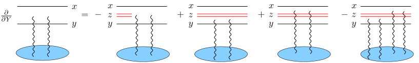
Figure 1: The diagrammatic representation of the BK-equation for dipole-hadron scattering.

One of the main results following from the BK-equation is the geometric scaling behaviour of the $T$-matrix [3, 4, 5] in a large kinematical window

$$T(r,Y)=T(r^{2}\,Q^{2}_{s}(Y))\ ,$$ (2)

where $Q_{s}(Y)$ is the so-called saturation momentum defined such that $T(r\simeq 1/Q_{s},Y)$ be of ${\cal{O}}(1)$. Eq. (2) means that the $T$-matrix scales with a single quantity $r^{2}\,Q^{2}_{s}(Y)$ rather than depending on $r$ and $Y$ separatelly. This behaviour implies a similar scaling for the DIS cross section, $\sigma^{\gamma^{*}p}(Y,Q^{2})=\sigma^{\gamma^{*}p}(Q^{2}/Q^{2}_{s}(Y))$, which is supported by the HERA data [7].

Another important result that can be extracted from the BK-equation is the rapidity dependence of the saturation momentum (leading-$Y$ contribution)[4, 5],

$$Q^{2}_{s}(Y)=Q_{0}^{2}\ \mbox{Exp}\left[\frac{2\alpha_{s}N_{c}}{\pi}\frac{\chi(\lambda_{0})}{1-\lambda_{0}}Y\right]\ ,$$ (3)

where $\chi(\lambda)$ is the BFKL kernel and $\lambda_{0}=0.372$.

The shape of the $T$-matrix resulting from the BK-equation is preserved in the transition region from weak ($T\simeq\alpha_{s}^{2}$) to strong ($T\simeq 1$) scattering with increasing $Y$, showing a “travelling wave” behaviour as sketched in Fig.2, on the left hand side. With increasing $Y$, the saturation region at $r\gg 1/Q_{s}(Y)$ where $T\simeq 1$ however widens up, including smaller and smaller dipoles, due to the growth of the saturation momentum. As we will see in the next sections, the situation changes a lot once gluon number fluctuations are taken into account.

2 Beyond the mean field approximation

2.0.1 Lorentz invariance and unitarity requirements

Let’s start with an elementary dipole of size $r_{1}$ at rapidity $y=0$ and evolve it using the BFKL evolution up to $y=Y$. The number density of dipoles of size $r_{2}$ at $Y$ in this dipole, $n(r_{1},r_{2},Y)$, obeys a completeness relation

$$n(r_{1},r_{2},Y)=\int\frac{d^{2}r}{2\pi r^{2}}\ n(r_{1},r,Y/2)\ n(r,r_{2},Y/2)\$$ (4)

where on the right hand side the rapidity evolution is separated in two successive steps, $y=0\to y=Y/2\to y=Y$. With

$$T(r_{1},r_{2},Y)\simeq c\ \alpha_{s}^{2}\ r_{2}^{2}\ n(r_{1},r_{2},Y)$$ (5)

eq.(4) can be approximately rewritten in terms of the $T$-matrix as

$$\left(\frac{1}{r_{2}^{2}}\ T(r_{1},r_{2},Y)\right)\simeq\ \frac{1}{2c\alpha_{s}^{2}}\ \int d\rho\ \ \left(\frac{1}{r^{2}}\ T(r_{1},r,Y/2)\right)\ \left(\frac{1}{r_{2}^{2}}\ T(r,r_{2},Y/2)\right)$$ (6)

where $\rho=\ln(r^{2}_{0}/r^{2})$. In Ref. [9] it was realized that the above completeness relations, or, equivalently, the Lorentz invariance, is satisfied by the BK evolution only by violating unitarity limits. This can be illustrated as follows: Suppose that $r_{2}$ is close to the saturation line, $r_{2}\simeq 1/Q_{s}(Y)$, so that the left hand side of Eq.(6) is large. On the right hand side of Eq.(6) it turns out that $T(r_{1},r,Y/2)/r^{2}$ is typically very small in the region of $\rho$ which dominates the integral. This means that $T(r,r_{2},Y/2)/r_{2}^{2}$ must be typically very large and must violate unitarity, $T(r,r_{2},Y/2)\gg 1$, in order to satisfy (6).

The simple procedure used in Ref. [9] to solve the above problem was to limit the region of the $\rho$-integration in Eq.(6) by a boundary $\rho_{2}(Y/2)$ so that $T(r,r_{2},Y/2)/r_{2}^{2}$ would never violate unitarity, or $T(r_{1},r,Y/2)/r^{2}$ would always be larger than $\alpha_{s}^{2}$. The main consequence of this procedure, i.e., BK evolution plus boundary correcting it in the weak scattering region, is the following scaling behaviour of the $T$-matrix near the unitarity limit

$$T(r,Y)=T\left(\frac{\ln(r^{2}Q_{s}^{2}(Y))}{\alpha_{s}Y/(\Delta\rho)^{3}}\right)$$ (7)

and the following energy dependence of the saturation momentum

$$Q_{s}^{2}(Y)=Q_{0}^{2}\ \mbox{Exp}\!\left[\frac{2\alpha_{s}N_{c}}{\pi}\frac{\chi(\lambda_{0})}{1-\lambda_{0}}Y\left(1-\frac{\pi^{2}\chi^{\prime\prime}(\lambda_{0})}{2(\Delta\rho)^{2}\chi(\lambda_{0})}\right)\right]$$ (8)

with

$$\Delta\rho=\frac{1}{1-\lambda_{0}}\ln\frac{1}{\alpha_{s}^{2}}+\frac{3}{1-\lambda_{0}}\ln\ln\frac{1}{\alpha_{s}^{2}}+\mbox{const.}\ .$$ (9)

Eq.(7) shows the breaking of the geometric scaling, which was the hallmark of the BK-equation shown in Eq.(2), and Eq.(8) shows the correction to the saturation momentum (cf. Eq.(3)), both emerging as a consequence of the evolution beyond the mean field approximation.

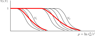
Figure 2: Left-hand side: The “travelling wave” behaviour of the solution to the BK-equation. Right-hand side: The $T$-matrix at two different rapidities, $Y_{1}$ and $Y_{2}$, for different events (thin lines). The thick lines represent the average over the events, $\langle T\rangle$, at the two rapidities, respectivelly. The shape of $\langle T\rangle$ becomes flatter with rising rapidity.

2.0.2 Statistical physics - high density QCD correspondence

The high energy evolution can be viewed also in another way which is inspired by dynamics of reaction-diffusion processes in statistical physics [10]. To show it, let’s consider an elementary target dipole of size $r_{1}$ which evolves from $y=0$ up to $y=Y$ and is then probed by an elementary dipole of size $r$, giving the amplitude $\bar{T}(r_{1},r,Y)$. It has become clear that the evolution of the target dipole is stochastic leading to random dipole number realizations inside the target dipole at $Y$, corresponding to different events in an experiment. The physical amplitude, $\bar{T}(r_{1},r,Y)$, is then given by averaging over all possible dipole number realizations/events, $\bar{T}(r_{1},r,Y)=\langle T(r_{1},r,Y)\rangle$, where $T(r_{1},r,Y)$ is the amplitude for dipole $r$ scattering off a particular realization of the evolved target dipole at $Y$. An illustration is shown in Fig.2, the right-hand side plot, where the $T$-matrix for different events (thin lines) and the average over all events (thick lines), $\langle T\rangle$, are shown at two different rapidities, respectivelly.

The mean field description breaks down at low target dipole occupancy due to the discreteness and the fluctuations of dipole numbers. Because of discreteness the dipole occupancy can not be less than one for any dipole size. Taking this fact into account by using the BK equation with a cutoff when $T$ becomes of order $\alpha^{2}_{s}$ [10], or the occupancy of order one (see Eq.(5)), leads exactly to the same correction for the saturation momentum as given in Eq.(3). The latter cutoff is essentially the same as, and gives a natural explanation of, the boundary used in Ref.[9] and briefly explained in the previous section.

The dipole number fluctuations in the low dipole occupancy region result in fluctuations of the saturation momentum from event to event, with the strength

$$\sigma^{2}=\langle\rho_{s}^{2}\rangle-\langle\rho_{s}\rangle^{2}\propto\frac{\alpha_{s}Y}{(\Delta\rho)^{3}}\$$ (10)

extracted from numerical simulations of statistical models. The averaging over all events with random saturation momenta, in order to get the physical amplitude, causes the breaking of the geometric scaling and replaces it by a new scaling law, the so-called diffusive scaling, in which case the scattering amplitude is a function of another variable,

$$\langle T(r,Y)\rangle=f\left(\frac{\ln(r^{2}Q_{s}^{2}(Y))}{\sqrt{\alpha_{s}Y/(\Delta\rho)^{3}}}\right)\ .$$ (11)

This equation differs from Eq.(7) since Eq.(7) misses dipole number fluctuations. Note that because of the geometric scaling violation, the result in Eq.(11) changes the shape as the rapidity increases, as illustrated in Fig. 2 (right-hand side) by the decreasing slope of the thick line with growing rapidity, in contrast to the solution to the BK-equation in Eq.(2).

The statistical physics/high-density QCD correspondence suggests the following picture for the wavefunction of a highly evolved hadron which is probed by a dipole of transverse size $r$: As the hadron is boosted to high rapidities the density of gluons inside the hadron grows. Also the fluctuation in gluon numbers, which is characterized by the dispersion in Eq. (10), grows with rising rapidity. However, as long as $\sigma^{2}\ll 1$, which means $Y\ll Y_{DS}\simeq\ (\Delta\rho)^{3}/\alpha_{s}$, the effects of fluctuations can be neglected and the evolution of the hadron is described to a good approximation by the BK-equation. Thus, for $Y\ll Y_{DS}$, as shown in Fig.3, to the left of the saturation line, $\rho\ll\langle\rho_{s}(Y)\rangle=\langle\ln(Q_{s}^{2}(Y)\,r_{0}^{2})\rangle$, is the “saturation region” with the “large-size” (small momentum) gluons at a large density, of order $1/\alpha_{s}$ or the $T\simeq 1$, while the shadowed region is the transition region from high to low gluon density, or the front of the at $T$-matrix (geometric scaling regime). At higher rapidities, $Y\gg Y_{DS}$, where the fluctuations become important, the geometric scaling regime is replaced by the diffusive scaling given in Eq. (11).

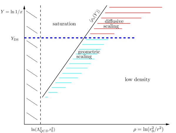
Figure 3: The phase diagram of the wavefunction of a highly evolved hadron.

2.0.3 Pomeron loop equations

It was always clear that the BK equation does not include fluctuations. However, it took some time to realize that also the Balitsky-JIMWLK equations do miss them. It turned out (see first Reference in [14]) that the Balitsky-JIMWLK equations do include BFKL evolution, “pomeron mergings” but not also “pomeron splittings”, which are represented by the three graphs in Fig. 4 for two dipoles scattering off a target, respectivelly. After this insight, the so-called Pomeron loop equations [13, 14] have been constructed to account for “pomeron splittings” or dipole number fluctuations.

The Pomeron loop equations can be expressed in a Hamiltonian language, in which case one extends the JIMWLK-equation [13], or in terms of scattering amplitudes [14], in which case the Balitsky equations are extended. In order to be close to the BK-equation discussed in sec. 1.1, we show the Pomeron loops using the scattering amplitude. In the large-$N_{c}$ limit, they can be written either as a stochastic equation of Langevin-type,

$$\frac{\partial T_{\bf xy}}{\partial Y} = \frac{\alpha_{s}N_{c}}{2\pi^{2}}\int\limits_{\bf z}\ M_{\bf xyz}\,\left[-T_{\bf xy}+T_{\bf xz}+T_{\bf zy}-T_{\bf xz}\,T_{\bf zy}\right]$$ (12)

$$+ \frac{\alpha_{s}}{2\pi}\sqrt{\frac{\alpha_{s}N_{c}}{2\pi^{2}}}\int\limits_{{\bf u,v,z}}{\cal A}({\bf x},{\bf y}|{\bf u},{\bf z})\frac{|{\bf u}-{\bf v}|}{({\bf u}-{\bf z})^{2}}\sqrt{\nabla^{2}_{\bf u}\nabla^{2}_{\bf v}\,T_{\bf uv}}\ \nu({\bf u},{\bf v},{\bf z};Y)$$

or, equivalently, as a hierarchy of coupled equations of averaged amplitudes, where for simplicity we show only the first two of them, which read

$$\frac{\partial\langle T_{\bf xy}\rangle}{\partial Y} = \frac{\alpha_{s}N_{c}}{2\pi^{2}}\int\limits_{\bf z}\ M_{\bf xyz}\,\left[-\langle T_{\bf xy}\rangle+\langle T_{\bf xz}\rangle+\langle T_{\bf zy}\rangle-\langle T_{\bf xz}\,T_{\bf zy}\rangle\right]$$

$$\frac{\partial\langle T_{\bf xz}T_{\bf zy}\rangle}{\partial Y} = \frac{\alpha_{s}N_{c}}{2\pi^{2}}\int\limits_{{\bf t}}\ M_{{\bf xzt}}\,\left[-\langle T_{\bf xz}T_{\bf zy}\rangle+\langle T_{\bf xt}T_{\bf zy}\rangle+\langle T_{\bf tz}T_{\bf zy}\rangle-\langle T_{\bf xt}\,T_{\bf tz}T_{\bf zy}\rangle\right]$$ (13)

$$+ \frac{\alpha_{s}N_{c}}{2\pi^{2}}\int\limits_{\bf t}\ M_{\bf zyt}\,\left[-\langle T_{\bf xz}T_{\bf zy}\rangle+\langle T_{\bf xz}T_{\bf zt}\rangle+\langle T_{\bf xz}T_{\bf ty}\rangle-\langle T_{\bf xz}\,T_{\bf zt}T_{\bf ty}\rangle\right]$$

$$+ \left(\frac{\alpha_{s}}{2\pi}\right)^{2}\frac{\alpha_{s}N_{c}}{2\pi^{2}}\ \int\limits_{{\bf u},{\bf v}}{\cal R}({\bf x},{\bf z},{\bf z},{\bf y}|{\bf u},{\bf v})\ \langle T_{\bf uv}\rangle$$

where the noise is non-diagonal (non-Gaussian) in the first two arguments

$$\langle\nu({\bf u}_{1},{\bf v}_{1},{\bf z}_{1};Y)\nu({\bf u}_{2},{\bf v}_{2},{\bf z}_{2};Y^{\prime})\rangle=\delta_{{\bf u}_{1}{\bf v}_{2}}\ \delta_{{\bf u}_{2}{\bf v}_{1}}\ \delta_{{\bf z}_{1}{\bf z}_{2}}\ \delta_{YY^{\prime}}\$$ (14)

the triple Pomeron kernel [43] reads

$${\cal R}({\bf x}_{1},{\bf y}_{1},{\bf x}_{2},{\bf y}_{2}|{\bf u},{\bf v})=\int\limits_{\bf z}\nabla^{2}_{\bf u}\nabla^{2}_{\bf v}\,\left[M_{\bf uvz}\,{\cal A}({\bf x}_{1},{\bf y}_{1}|{\bf u},{\bf z})\,{\cal A}({\bf x}_{2},{\bf y}_{2}|{\bf z},{\bf v})\right]$$ (15)

and $\alpha_{s}^{2}{\cal A}$ is the amplitude for dipole-dipole scattering in the two-gluon exchange approximation and for large-$N_{c}$, with

$${\cal A}({\bf x},{\bf y}|{\bf u},{\bf v})=\frac{1}{8}\ \ln^{2}\left[\frac{({\bf x}-{\bf v})^{2}\,({\bf y}-{\bf u})^{2}}{({\bf x}-{\bf u})^{2}\,({\bf y}-{\bf v})^{2}}\right]\ .$$ (16)

In above equations the integrations are always over transverse sizes, $\int_{{\bf x},{y}}=d^{2}x\ d^{2}y$.

Last term in Eq.(12), containing the non-Gaussian noise $\nu$, is new as compared with the BK-equation and accounts for fluctuations in the dipole numbers or the stochastic nature of the evolution in small-$x$ physics. The hierarchy in Eq.(13) reduces to the BK-equation only in the mean field approximation, i.e., when $\langle T\,T\rangle=\langle T\rangle\langle T\rangle$. The hierarchy in Eq.(13), as compared with the Balitsky-JIMWLK hierarchy, involves in addition to linear BFKL evolution (Fig.4(a)) and pomeron mergings (Fig.4(b)), also pomeron splittings (Fig.4(c)), and therefore, in the course of the evolution, also pomeron loops. The three pieces of evolution are represented by the linear terms, nonlinear terms and the last term on the right-hand side of the second equation in Eq.(13), respectivelly, which describes the scattering of two dipoles off a target.

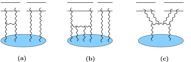
Figure 4: Two dipoles scattering off a hadron: (a) BFKL interaction, (b) “pomeron mergings”, (c) “pomeron splittings”.

2.0.4 Phenomenology

It isn’t yet clear at which energy fluctuation/Pomeron loop effects start becoming important. The results shown in the previous sections, Eq.(8) and Eq.(11), are valid at asymptotic energies. A solution to the evolution equations, which is not yet available because of their complexity, would have helped to better understand the subasymptotics.

Using the statistical physics/high density QCD correspondence, phenomenological consequences of fluctuations in the fixed coupling case have been studied, for example for DIS and diffractive cross sections [20], forward gluon production in hadron-hadron collisions [21] and for the nuclear modification factor $R_{p}A$ [17], in case fluctuations become important in the range of LHC energies. Recently, in the fixed coupling case, it has been shown that dipole-proton scattering amplitudes which include fluctuation effects seem to describe better the HERA data. Also the parameters turn out reasonable: The diffusion coefficient $D\simeq 0.35$ ($\sigma^{2}=D\,Y$) is in agreement with numerical simulations of approximations to Pomeron loop equations [27, 36] and the saturation exponent $\lambda\simeq 0.2$ ($Q_{s}^{2}=(x_{0}/x)^{\lambda}$) is decreased as expected theoretically. On the other hand, allowing the coupling to run, however, within a toy model [36] which is supposed to mimic the QCD evolution equations with Pomeron loops, it has been argued that gluon number fluctuations/pomeron loops can be neglected in the range of HERA and LHC energies. See also Refs. [9, 44] for more studies on running coupling plus gluon number fluctuations.

References

- [1] Y. V. Kovchegov, Phys. Rev. D60, 034008 (1999)
- [2] I. Balitsky, Nucl. Phys. B463, 99 (1996)
- [3] E. Iancu, K. Itakura, and L. McLerran, Nucl. Phys. A708, 327 (2002)
- [4] A. H. Mueller and D. N. Triantafyllopoulos, Nucl. Phys. B640, 331 (2002)
- [5] S. Munier and R. Peschanski, Phys. Rev. Lett. 91, 232001 (2003)
- [6] S. Munier and R. Peschanski, Phys. Rev. D69, 034008 (2004)
- [7] A. M. Stasto, K. J. Golec-Biernat, and J. Kwiecinski, Phys. Rev. Lett. 86, 596 (2001). hep-ph/0007192
- [8] D. N. Triantafyllopoulos, Nucl. Phys. B648, 293 (2003)
- [9] A. H. Mueller and A. I. Shoshi, Nucl. Phys. B692, 175 (2004)
- [10] E. Iancu, A. H. Mueller, and S. Munier, Phys. Lett. B606, 342 (2005)
- [11] E. Iancu and R. Venugopalan (2003). hep-ph/0303204
- [12] H. Weigert, Prog. Part. Nucl. Phys. 55, 461 (2005)
- [13] A. H. Mueller, A. I. Shoshi, and S. M. H. Wong, Nucl. Phys. B715, 440 (2005)
- [14] E. Iancu and D. N. Triantafyllopoulos, Nucl. Phys. A756, 419 (2005)
- [15] E. Iancu and D. N. Triantafyllopoulos, Phys. Lett. B610, 253 (2005)
- [16] A. Kovner and M. Lublinsky, Phys. Rev. D71, 085004 (2005)
- [17] M. Kozlov, A. I. Shoshi, and B.-W. Xiao, Nucl. Phys. A792, 170 (2007)
- [18] M. Kozlov, A. I. Shoshi, and B.-W. Xiao (2007). arXiv:0706.3998 [hep-ph]
- [19] M. Kozlov, A. Shoshi, and W. Xiang (2007). arXiv:0707.4142 [hep-ph]
- [20] Y. Hatta, E. Iancu, C. Marquet, G. Soyez, and D. N. Triantafyllopoulos, Nucl. Phys. A773, 95 (2006)
- [21] E. Iancu, C. Marquet, and G. Soyez, Nucl. Phys. A780, 52 (2006)
- [22] A. Dumitru, E. Iancu, L. Portugal, G. Soyez, and D. N. Triantafyllopoulos (2007). arXiv:0706.2540 [hep-ph]
- [23] A. Kovner and M. Lublinsky, Phys. Rev. Lett. 94, 181603 (2005)
- [24] A. Kovner and M. Lublinsky, Phys. Rev. D72, 074023 (2005)
- [25] C. Marquet, A. H. Mueller, A. I. Shoshi, and S. M. H. Wong, Nucl. Phys. A762, 252 (2005)
- [26] J. P. Blaizot, E. Iancu, K. Itakura, and D. N. Triantafyllopoulos, Phys. Lett. B615, 221 (2005)
- [27] G. Soyez, Phys. Rev. D72, 016007 (2005)
- [28] R. Enberg, K. J. Golec-Biernat, and S. Munier, Phys. Rev. D72, 074021 (2005)
- [29] E. Brunet, B. Derrida, A. H. Mueller, and S. Munier, Europhys. Lett. 76, 1 (2006)
- [30] E. Brunet, B. Derrida, A. H. Mueller, and S. Munier, Phys. Rev. E73, 056126 (2006)
- [31] C. Marquet, G. Soyez, and B.-W. Xiao, Phys. Lett. B639, 635 (2006)
- [32] A. I. Shoshi and B.-W. Xiao, Phys. Rev. D73, 094014 (2006)
- [33] A. I. Shoshi and B.-W. Xiao, Phys. Rev. D75, 054002 (2007)
- [34] S. Bondarenko, L. Motyka, A. H. Mueller, A. I. Shoshi, and B. W. Xiao, Eur. Phys. J. C50, 593 (2007)
- [35] J. P. Blaizot, E. Iancu, and D. N. Triantafyllopoulos, Nucl. Phys. A784, 227 (2007)
- [36] E. Iancu, J. T. de Santana Amaral, G. Soyez, and D. N. Triantafyllopoulos, Nucl. Phys. A786, 131 (2007)
- [37] S. Munier, Phys. Rev. D75, 034009 (2007)
- [38] M. Kozlov and E. Levin, Nucl. Phys. A779, 142 (2006)
- [39] M. Kozlov, E. Levin, V. Khachatryan, and J. Miller, Nucl. Phys. A791, 382 (2007)
- [40] E. Levin and A. Prygarin (2007). hep-ph/0701178
- [41] M. A. Braun and G. P. Vacca, Eur. Phys. J. C50, 857 (2007)
- [42] A. H. Mueller, Nucl. Phys. B415, 373 (1994)
- [43] M. A. Braun and G. P. Vacca, Eur. Phys. J. C6, 147 (1999)
- [44] G. Beuf (2007). arXiv:0708.3659 [hep-ph].