MPI for Dynamics and Self-Organization, Bunsenstraße 10, D-37073 Göttingen, Germany
Physikalisches Institut, Albert-Ludwigs-Universität, Hermann-Herder-Str. 3, D-79104 Freiburg, Germany
Department of Physics, Ben-Gurion University, Beer-Sheva 84105, Israel
Control of atomic currents using a quantum stirring device
Abstract
We propose a BEC stirring device which can be regarded as the incorporation of a quantum pump into a closed circuit: it produces a DC circulating current in response to a cyclic adiabatic change of two control parameters of an optical trap. We demonstrate the feasibility of this concept and point out that such device can be utilized in order to probe the interatomic interactions.
pacs:
03.65.-wpacs:
03.65.Vfpacs:
05.30.JpQuantum mechanics. Phases: geometric; dynamic or topological. Boson systems.
The realization of Bose-Einstein Condensation (BEC) of ultra-cold atoms in optical lattices and atom chips [1] and the availability of conveyor belts [2] is considered to be a major breakthrough with potential applications in the arena of quantum information processing [3], atom interferometry [4, 5, 6], lasers [1, 7] and atom diodes and transistors [8, 9, 10]. A major advantage of BEC based devices, as compared to conventional solid-state structures, lies in the extraordinary degree of precision and control that is available, regarding not only the confining potential, but also the strength of the interatomic interactions, their preparation and the measurement of the atomic cloud. Accordingly it is envisioned that the emerging field of “atomtronics” will provide a new generation of nanoscale devices.
The possibility to induce DC currents by periodic (AC) modulation of the potential is
familiar from the context of electronic devices. If an open geometry is concerned, it
is known as “quantum pumping” [11] ,
while for closed geometries we use the term “quantum stirring” [12].
We consider below the stirring of condensed ultra-cold atoms
due to the periodic variation of the on-site potentials
and of the tunneling rates between adjunct confining traps.
We show that the nature of the transport process depends crucially
on the sign and on the strength of the interatomic interactions.
We distinguish between four regimes of dynamical behavior:
For strong repulsive interaction the particles
are transported one-by-one, which we call sequential crossing;
for weaker repulsive interaction we
observe either gradual crossing or coherent mega crossing;
finally, for strong attractive interaction the particles
move together as one composite unit from trap to trap.
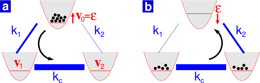
Model – The simplest model that captures the physics of quantum stirring is the three-site Bose-Hubbard Hamiltonian (BHH) [14, 13, 10, 15] (see Fig. 1) 111 The three-site BHH is a prototype system for many recent studies [13]. A classical analysis of this system was performed in [15] where it was shown that for appropriate system parameters and initial conditions chaotic dynamics would emerge. In this work we consider adiabatic driving of ground state preparation and therefore chaotic motion is not an issue.. We call the site “gated-well” since we late assume that we have control over its potential energy . The sites form a two level “double-well” with potential energy . The boson BHH is:
| (1) |
We set which corresponds to measuring energies in units of frequency. Furthermore, without loss of generality we choose time units such that . Accordingly the two single particle levels of the double-well are . The annihilation and creation operators and obey the canonical commutation relations while the operators count the number of bosons at site . The interaction strength between two atoms in a single site is given by where is the effective volume, is the atomic mass, and is the -wave scattering length which can be changed by applying an additional magnetic field [16]. The on-site potentials as well as the coupling strengths are controlled by changing the confining potential. The main assumption underlying the BHH is that the single-particle ground state wavefunctions are sufficiently localized at the sites, and that for the temperatures involved they are well separated in energy from the excited single-particle levels. Experimentally, such deep trapping potentials can accommodate several hundred particles[17].
The couplings between the gated-well and the two ends of the double-well are and . We
assume that both are much smaller than (for the two-mode BEC dynamics see for
example [18]).
It is convenient to define the two control parameters of the pumping
as and .
By periodic cycling of the parameters
we can obtain a non-zero amount () of transported atoms per cycle.
The pumping cycle is illustrated in Figs. 1,2.
Initially all the particles are located in the gated-well
which has a sufficiently
negative on-site potential energy ().
In the first half of the cycle the coupling is biased in favor of
the route () while is raised
until (say) the gated-well is empty
222Later we estimate the required variation
in order to have all the particles transferred from
the gated-well to the double well. We also analyze smaller
pumping cycles (see Fig. 3b) for which only a fraction
of particles gets through..
In the second half of the cycle the coupling
is biased in favor of the route (), while is
lowered until the gated-well is full.
Assuming , the gated-well is depopulated via the route
into the lower energy level
during the first half of the cycle, and re-populated
via the route during the second half of the cycle.
Accordingly the net effect is to have a non-zero .
If we had a single particle in the system,
the net effect would be to pump roughly one particle
per cycle. If we have non-interacting particles,
the result of the same cycle is to pump
roughly particles per cycle
333
Through the driving cycle the total number of bosons remains constant.
The energy is not a constant of motion, but in the adiabatic limit
the system comes back to the same state at the end of each cycle..
We would like to know what is the actual result using
a proper quantum mechanical calculation,
and furthermore we would like to investigate what is the
effect of the interatomic interaction on the result.
Methods – Within the framework of linear response theory the induced current is if we change and if we change . The coefficients and in these linear relations are defined as the elements of the geometric conductance matrix, and can be calculated using the Kubo formula approach (see below). Integrating the current over a full cycle we get
| (2) |
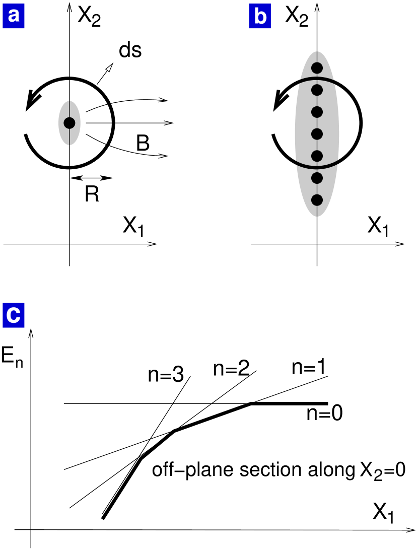
In order to calculate the geometric conductance we use the Kubo formula approach to quantum pumping [19] which is based on the theory of adiabatic processes [20]. It turns out that in the strict adiabatic limit is related to the vector field in the theory of the Berry phase which is known as the “Berry Curvature”. The adiabatic slowness condition on in the present context, taking into account the two-orbital approximation, is discussed in Section 4 of [21]. Using the notations and it is illuminating to rewrite Eq.(2) as
| (3) |
where we define the normal vector as illustrated in Fig. 2. The calculation of the so-called Kubo-Berry Curvature is done using the following formula [19]:
| (4) |
Above is the averaged current 444Due to the continuity equation the same result for is obtained irrespective of whether we measure the current via the bond or via the bond. The advantage of using the the “symmetrized” version for is that the same amount of particles is being transported during both halves of the cycle, allowing us to focus on (say) the first half and then double the result. via the bonds and , while is the generalized force associated with the control parameter . The index labels the eigenstates of the many-body Hamiltonian. We assume from now on that is the BEC ground state11footnotemark: 1.
The advantage of the above, so called “geometric”
point of view is in the intuition that it gives
for the result:
Formally the field is like a
projection of a fictitious magnetic field in an embedding
three-dimensional space (the third coordinate
if formally defined such that ).
The flux of this fictitious magnetic field through any out-of-plane
surface which is enclosed by the pumping cycle
gives the so-called Berry phase, while the line integral over this
fictitious magnetic field, i.e. Eq.(3) 555In the plane the
third component of the fictitious magnetic field is zero due to the
time-reversal symmetry [19]., gives . As implied by inspection
of Eq.(4) the sources of are located
at points where the ground level has a degeneracy
with the next level. A simple argument implies
that this “magnetic charge” is quantized like Dirac monopoles,
else the Berry phase would be ill-defined.
For details see [19].
In our model system for all the “magnetic charge”
is concentrated in one point. As the interaction
becomes larger the -fold degeneracy of the levels
is lifted, and this “magnetic charge” disintegrates
into elementary “monopoles” (see Fig. 2).
We further discuss the energy spectrum in the next section.
Regimes – We define the average coupling as . In the zeroth-order approximation and are neglected, and later we take them into account as a perturbation. For the number () of particles in the gated-well becomes a good quantum number hence we can associate the level index with the number of particles in the gated-well. Furthermore, we adopt a “two-orbital approximation”: we assume that there is non-zero occupation only in the gated-well and in the lower double-well level, which is valid if . Note also that we assume an adiabatic process33footnotemark: 3, and accordingly non-adiabatic transitions to the higher orbitals can be safely neglected [21].

Within the two-orbital approximation the many body energies are , where , and , and . The location of the crossing is determined from the degeneracy condition , where . The crossings are distributed within . The rescaled version of the control variable is , and its support is . The distance between the crossings, while varying the gated-well potential , is . Once we take into account we get avoided crossings of width . If is large these avoided crossings merge and eventually we get one mega crossing.
For the purpose of further analysis we
apply the two-orbital approximation,
within which the many body Hamiltonian matrix
is ,
where and the couplings are defined
as . The calculation involves
the matrix elements of , leading to .
Analogous expression applies to the current operator where
is replaced by .
For large , as is varied,
we encounter (say for ) a sequence of distinct Landau-Zener transitions
().
The distance between avoided crossings
is of order while their width
is .
The widest crossings are at the center with .
This should be contrasted with
the energy scales and
that describe the span of the crossings.
Accordingly we deduce that for repulsive
interaction there are three distinct regimes:
for we have a “mega crossing”;
for we have the “sequential crossing regime”,
while in the intermediate regime we have a “gradual crossing”.
Below we summarize the
results in the various regimes. In particular
Eq.(7) is obtained from Eq.(4)
with a two level approximation for each crossing.
We also related briefly to the regime.
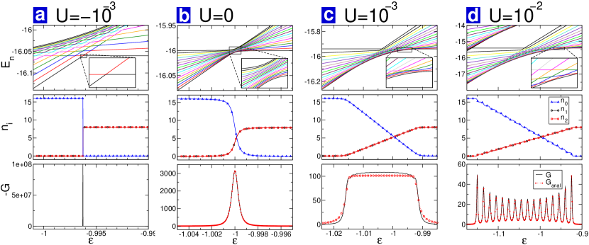
Results – Most of the contribution to the line integral in Eq.(2) comes as we change during the avoided crossings that have been discussed in the previous section. If we close the pumping cycle outside of this limited range, then the -variation can be safely neglected. Accordingly we refer from now on to only. An overview of the numerical results for the conductance is shown in Fig. 3, where we plot as a function of for various interaction strengths . In the same figure we report the normalized amount of particles for various driving cycles. As the shape of changes, the dependence of on the -span of the pumping cycle becomes of importance. Thus, by measuring we obtain information on the strength of the interatomic interactions.
In Fig. 4 more details are presented: besides we also plot the -dependence of the energy levels, and of the site population. Four representative values of are considered including also the case. Let us discuss the observed results. For all the particles cross “together” from the gated-well orbital to the double-well orbital. We call this type of dynamics “mega crossing”. The outcome is just times the single particle result:
| (5) |
which can be expressed in terms of the control parameters . This result approximately hold as long as . Integrating over a full cycle one obtains
| (6) |
where is the radius of the pumping cycle (see Fig. 2). For small cycles we get , while for large cycles we get the limiting value . In the other extreme, for very repulsive interaction () we get
| (7) |
For intermediate values , we find neither the sequential crossing of Eq.(7), nor the mega-crossing of Eq.(5), but rather a gradual crossing. Namely, in this regime, over a range we get a constant geometric conductance:
| (8) |
which reflects in a simple way the interaction strength. This formula was deduced by extrapolating Eq.7, and then was validated numerically (lower panel of Fig. 4c).
As discussed above for large positive
the -fold “degeneracy” of
the Landau-Zener crossing is lifted,
and we get a sequence of Landau-Zener crossings
(for schematic illustration see the lower panel of Fig. 2,
and compare with the numerical results in the upper panels of Fig. 4).
Also for this -fold “degeneracy” is lifted,
but in a different way: the levels separate in the “vertical” (energy) direction
rather than “horizontally” (see upper panels of Fig. 4).
Accordingly all the particles execute a single two-level transition
from the gated-well to the double-well (see Fig. 4a).
This direct Landau-Zener transition from the level
to the level is very sharp because it is mediated
by an -th order virtual transition via the intermediate states.
Accordingly, for sufficiently strong attractive interaction
all the particles move together from the gated-well to
one of the double-well sites. When the sign of is reversed they are
transported from one end of the double-well to the other end (not shown).
This should be clearly distinguished from the -fold degenerated transition
to the lower double-well level which is observed in the case.
Summary – The theoretical [10, 18, 22] and experimental [23] study of driven dynamics in single and double site systems is the state of the art. Study of three-site systems adds the exciting topological aspect: controlled atomic current can be induced using optical lattice technology [24]. The actual measurement of induced neutral currents poses a challenge to experimentalists. In fact there is a variety of techniques that have been proposed for this purpose. For example one can exploit the Doppler effect in the perpendicular direction, which is known as the rotational frequency shift [25]. The analysis of the prototype trimer system reveals the crucial importance of interactions. The interactions are not merely a perturbation: rather they determine the nature of the transport process. We expect the induced circulating atomic current to be extremely accurate, which would open the way to various applications, either as a new metrological standard, or as a component of a new type of quantum information or processing device.
Acknowledgements.
This research was supported by a grant from the United States-Israel Binational Science Foundation (BSF) and the DFG (Forschergruppe 760).References
- [1] B.P. Anderson et al. , Science 282, 1686 (1998). D. Jaksch et al., Phys. Rev. Lett. 81, 3108 (1998). C. Orzel et al., Science 291, 2386 (2001). M. Greiner et al., Nature 415, 39 (2002). I. Bloch, Nature Phys. 1, 23-30 (2005) R. Folman et al., Phys. Rev. Lett. 84, 4749 (2000).
- [2] W. Hansel, et al., Nature 413, 498 (2001); W. Hansel, et al., New J. Phys. 7, 3 (2005).
- [3] J. Schmiedmayer, R. Folman, T. Calarco, J. Mod. Opt. 49, 1375 (2002).
- [4] T. Schumm, et al., Nat. Phys. 1, 57 (2005).
- [5] Y-J Wang, et al., Phys. Rev. Lett. 94, 090405 (2005); E. Andersson, et al., Phys. Rev. Lett. 88, 100401 (2002).
- [6] M. R. Andrews, et al., Science 275, 637 (1997).
- [7] M. O. Mewes, et al., Phys. Rev. Lett. 78, 582 (1997); E. W. Hagley, et al., Science 283, 1706 (1999); Y. Shin, et al., Phys. Rev. Lett. 92, 050405 (2004).
- [8] A. Micheli, et al., Phys. Rev. Lett. 93, 140408 (2004).
- [9] B. T. Seaman, et al., (2006) [cond-mat/0606625].
- [10] J. A. Stickney, D. Z. Anderson, A. A. Zozulya, Phys. Rev. A 75, 013608 (2007).
- [11] D. J. Thouless, Phys. Rev. B 27 6083 (1983). Q. Niu and D. J. Thouless, J. Phys. A 17 2453 (1984). M. Buttiker, H. Thomas and A Pretre, Z. Phys. B-Condens. Mat., 94, 133-137 (1994). P. W. Brouwer, Phys. Rev. B 58, R10135 (1998). B. L. Altshuler, L. I. Glazman, Science 283, 1864 (1999). M. Switkes, et al., Science 283, 1905 (1999).
- [12] G. Rosenberg and D. Cohen, J. Phys. A 39, 2287 (2006), and further references therein.
- [13] M. Hiller, T. Kottos, and T. Geisel, Phys. Rev. A 73, 061604(R) (2006), and further references therein.
- [14] J. D. Bodyfelt, M. Hiller, and T. Kottos, Europhys. Lett. 78, 50003 (2007).
- [15] R. Franzosi, V. Penna, Phys. Rev. E 67, 046227 (2003); K. Nemoto, et al., Phys. Rev. A 63, 013604 (2000).
- [16] A. J. Legget, Rev. Mod. Phys. 73, 307 (2001).
- [17] G. J. Milburn, J. Corney, E. M. Wright, and F. D. Walls, Phys. Rev. A. 55, 4318 (1997).
- [18] M. Jääskeläinen, P. Meystre, Phys. Rev A 73, 013602 (2006); D. R. Dounas-Frazer, L. D. Carr, quant-ph/0610166 (2006); K. W. Mahmud, H. Perry, W. P. Reinhardt, J. Phys. B 36, L265 (2003); M. Albiez et al., Phys. Rev. Lett. 95, 010402 (2005).
- [19] D. Cohen, Phys. Rev. B 68, 155303 (2003).
- [20] M.V. Berry, Proc. R. Soc. Lond. A 392, 45 (1984). J.E. Avron, A. Raveh and B. Zur, Rev. Mod. Phys. 60, 873 (1988). M.V. Berry and J.M. Robbins, Proc. R. Soc. Lond. A 442, 659 (1993).
- [21] M. Chuchem and D. Cohen, J. Phys. A 41, 075302 (2008).
- [22] B. Wu and J. Liu, Phys. Rev. Lett. 96, 020405 (2006); J. Liu, B. Wu, Q. Niu, Phys. Rev. Lett. 90, 170404 (2003).
- [23] C.-S. Chuu, et. al, Phys. Rev. Lett. 95, 260403 (2005); A. M. Dudarev, M. G. Raizen, and Q. Niu, Phys. Rev. Lett. 98, 063001 (2007).
- [24] L. Amico, A. Osterloh, F. Cataliotti, Phys. Rev. Lett. 95, 063201 (2005).
- [25] I. Bialynicki-Birula and Z. Bialynicka-Birula, Phys. Rev. Lett. 78, 2539 (1997).