The evolution of planetary nebulae

Abstract

Context. The luminosity function of planetary nebulae, in use for about two decades in extragalactic distance determinations, is still subject to controversial interpretations.

Aims. The physical basis of the luminosity function is investigated by means of several evolutionary sequences of model planetary nebulae computed with a 1D radiation-hydrodynamics code.

Methods. The nebular evolution is followed from the vicinity of the asymptotic-giant branch across the Hertzsprung-Russell diagram until the white-dwarf domain is reached, using various central-star models coupled to different initial envelope configurations. Along each sequence the relevant line emissions of the nebulae are computed and analysed.

Results. Maximum line luminosities in H$\beta$ and [O iii] 5007 Å are achieved at stellar effective temperatures of about 65 000 K and 95 000…100 000 K, respectively, provided the nebula remains optically thick for ionising photons. In the optically thin case, the maximum line emission occurs at or shortly after the thick/thin transition. Our models suggest that most planetary nebulae with hotter ($\ga 45\,000$ K) central stars are optically thin in the Lyman continuum, and that their [O iii] 5007 Å emission fails to explain the bright end of the observed planetary nebulae luminosity function. However, sequences with central stars of $\ga\!0.6$ M_☉ and rather dense initial envelopes remain virtually optically thick and are able to populate the bright end of the luminosity function. Individual luminosity functions depend strongly on the central-star mass and on the variation of the nebular optical depth with time.

Conclusions. Hydrodynamical simulations of planetary nebulae are essential for any understanding of the basic physics behind their observed luminosity function. In particular, our models do not support the claim of Marigo et al. (2004) according to which the maximum 5007 Å luminosity occurs during the recombination phase well beyond 100 000 K when the stellar luminosity declines and the nebular models become, at least partially, optically thick. Consequently, there is no need to invoke relatively massive central stars of, say $>\!0.7$ M_☉, to account for the bright end of the luminosity function.

1 Introduction

Since the pioneering paper by Jacoby (1989) in which the theoretical fundament of the planetary nebulae luminosity function (PNLF) has been laid out, the use of this tool for establishing cosmic distances has been proven to be extremely successful. Its main success stems from the fact that it works not only for spirals, but also for ellipticals, despite the fact that both systems consists of completely different stellar populations. A recent summary of the use of the PNLF can be found in Ciardullo (2003, and references therein).

Jacoby (1989) defined the line magnitudes as

$$m=-2.5\,\log F-13.74\,,$$ (1)

with $F$ (in erg cm^-2 s^-1) being the line flux from the object. Based on 13 galaxies with well-determined Cepheid distances, an absolute cut-off brightness of $M^{\star}(5007)=-4.45\pm 0.05$  mag has been derived (Ciardullo 2003). This brightness corresponds to 620 L_☉ emitted in the [O iii] 5007 Å line!

Despite its use for about two decades, the physical basis of the PNLF is still mysterious and subject to controversal interpretations. A major uncertainty is related to the question whether the brightest planetary nebulae (PNe) are optically thick or thin for Lyman continuum photons because the efficiency of converting stellar UV radiation into optical line emission is heavily dependent on the optical depth.

Jacoby (1989) considered only optically thick nebular models for the construction of a theoretical PNLF. Based on the post-asymptotic giant branch (post-AGB) tracks available, Jacoby computed the line luminosities from expanding filled spheres along tracks with hydrogen-burning and helium-burning central stars, and found, by comparing the brightest PNe in Local Group galaxies with these models, upper mass limits for central stars of $\approx\!0.65$ M_☉.

Also in the work of Dopita et al. (1992) for Magellanic Cloud PNe only optically thick nebular models were considered. These authors found that the maximum stellar luminosity belonging to the [O iii] cutoff is $\simeq\!10^{4}$ L_☉, corresponding to $\simeq\!0.7$ M_☉ if the standard core-mass luminosity relation of hydrogen-burning central stars is used.

Stanghellini (1995) modelled only the H$\beta$ luminosity function, assuming also optically thick nebulae, and investigated the dependence on star formation rate, post-AGB transition time and initial-final mass relation. The observed H$\beta$ cut-off at $\simeq\!-2.5$ mag was achieved by nebular models around nuclei with 0.65 M_☉ for a fairly broad range of assumptions.

Considering only models that are optically thick to ionising radiation oversimplifies the problem certainly. Thus Méndez et al. (1993) and Méndez & Soffner (1997) used a different method. They modelled luminosity functions based on hydrogen-burning post-AGB evolutionary tracks and empirical properties of PNe without resorting to nebular models. Their main conclusion is that the bright end of the luminosity function is predominantly populated by optically thin PNe (not thin in all directions around the central star, but thin in at least some directions to allow for some leaking of Lyman continuum photons) with maximum central-star masses between 0.63 and 0.66 M_☉.

A completely novel approach was introduced by Marigo et al. (2001, 2004). These authors constructed simple nebular models, taking into account their outer boundary conditions set by the AGB and the central-star winds, using analytical expressions for interacting winds in a similar way as described by Volk & Kwok (1985). The pressure increase within the nebular shell by photoionisation is approximately considered. This new “synthetic” approach allows to compute the evolution of model PNe together with their observable quantities in a very fast and efficient way.

Using their new tool, Marigo et al. (2004) computed nebular sequences along the post-AGB tracks of Vassiliadis & Wood (1994) and constructed PNLFs for stellar populations with various metallicities and star formation histories. It turned out that the bright end of the PNLF is populated by objects with central-star masses between 0.70 and 0.75 M_☉. Consequently, the value of the bright cut-off of the PNLF must depend critically on the properties of the parent stellar population: large differences between the maximum PNe luminosities of elliptical and spiral galaxies are to be expected (see Marigo et al. 2004, Fig. 25 therein), which, however, are not observed.

This completely different interpretation of the luminosity function prompted us to employ our hydrodynamical models presented in Perinotto et al. (2004, Paper I hereafter) to investigate the physical basis of the PNLF with a more realistic approach. We believe that hydrodynamical simulations are ideally suited to tackle this task since it has been demonstrated on several occasions that a reasonably good match to observed properties of PNe is achieved with such models, provided appropriate initial and boundary conditions are chosen (Schönberner et al. 1997; Schönberner & Steffen 1999, 2003a, 2003b; Steffen & Schönberner 2006). However, we do not aim at constructing a theoretical luminosity function because the number of available combinations of nebular models and central-star masses is too low. Instead, we will concentrate on a description of the processes responsible for the strength of the relevant line emissions.

We begin in Sect. 2 with a short description of our hydrodynamical modelling including a brief description of the evolutionary properties of PNe as they follow from these models. We outline in Sect. 3 the basic differences to the Marigo et al. approach and investigate in Sect. 4 in detail how the luminosities of important lines depend on the model properties and how they evolve with time. Section 5 is devoted to individual luminosity functions as predicted by our simulations. Section 6 introduces the corresponding H$\beta$ luminosity functions. The paper is closed by Sect. 7 with an extensive discussion. A short presentation of the basic results of this investigation has already been given by (Schönberner et al. 2006a).

2 Modelling the planetary nebulae evolution

A detailed description how we simulate the formation and evolution of planetary nebulae has already been given in previous papers and shall not be repeated here (Perinotto et al. 1998, 2004). Instead, we emphasise here only the basic ingredients of our calculations which are important for the general appreciation of our models and for understanding the differences to the “synthetic” approach of Marigo et al. (2001).

In this context it is important to remember that a planetary nebula is a very complex dynamical system, even if we approximate real objects by spherical configurations. The whole object consists of a rapidly evolving post-AGB star and an expanding circumstellar envelope originally set up by a massive stellar wind when the object was still on or close to the AGB. The radiation field and the wind from the central star initiate a shock wave pattern at the inner edge of the slowly expanding AGB wind envelope. Its structure and expansion properties depend mainly on the radial density distribution of the AGB material, on the electron temperature inside the ionised matter, and on the pressure support from the central-star wind. The PN proper is confined between an inner contact surface which separates the nebula matter from the shock-heated wind matter, and an outer shock front which propagates through the ambient AGB material, thereby increasing the PN mass with time.

Any approach with the aim to understand at least the basic physics of the formation and evolution of PNe must therefore rely on radiation-hydrodynamics simulations with the proper initial and boundary conditions, with all the relevant physical processes treated fully time-dependently.

2.1 The hydrodynamical models

In short, the basic philosophy of our hydrodynamical PN models is to couple a spherical circumstellar envelope, assumed to be the relic of a strong AGB wind, to a post-AGB model and to follow the evolution of the whole system across the Hertzsprung-Russell diagram towards the white-dwarf cooling path, employing an 1D radiation-hydrodynamics code (see Perinotto et al. 1998). We emphasize that our code is designed to compute ionisation, recombination, heating, and cooling fully time-dependently. For each volume element, the cooling function is composed of the contributions of all the ions considered (next to H and He, also C, N, O, Ne, S, Cl, and Ar). For each individual element up to 12 ionisation stages are taken into account. More details on the radiation part of our code can be found in Marten & Szczerba (1997).

We used in all of our computations a chemical composition typical for Galactic disk PNe (Table 1). Although the line emission of a PN and the luminosity and radiation field of its central star depend on the metal content, the effect is relatively small and will not influence the basic properties of the PNLF (cf. Dopita et al. 1992). Any abundance variations, notably that of oxygen, are thus not considered in the present work.

Table 1: Elemental abundances, $\epsilon_{\mathrm{i}}$, used in the computations of our hydrodynamical models, in (logarithmic) number fractions relative to hydrogen, $\log{\epsilon}_{\mathrm{i}}=\log n_{\mathrm{i}}/\log n_{\mathrm{H}}+12$.

H	He	C	N	O	Ne	S	Cl	Ar
12.00	11.04	8.89	8.39	8.65	8.01	7.04	5.32	6.46

The hydrodynamical model sequences selected for the present work from Paper I are listed in Table 2. The table provides the sequence numbers from Paper I (col. 1), the central-star masses (col. 2), the central-star luminosities at 30 000 K (col. 3), the AGB mass-loss rates (col. 4) and the AGB wind velocities (col. 5) of the initial models, and the envelope types (col. 6). The initial envelope models have either an ad hoc radial power-law density distribution, $\rho\propto r^{-2}$ (Type A), or are the result of detailed hydrodynamics simulations along the upper AGB (Type C), as described in Schönberner et al. (1997) or in Paper I. The structure of the Type C envelope reflects the mass-loss history of the preceding 50 000 years of AGB evolution while Type A corresponds to the simple case of constant mass loss and outflow velocity.

An additional stellar track was introduced in Schönberner et al. (2005a, Paper II hereafter) by replacing the 0.605 M_☉ track of sequence No. 6 by a 0.595 M_☉ track interpolated from the 0.605 M_☉ and 0.565 M_☉ tracks of Blöcker (1995) and Schönberner (1983). The PNe models of this new sequence (No. 6a in Table 2) match the observations even better than the models of sequence No. 6 with a 0.605 M_☉ central star (Schönberner et al. 2005b, Paper III hereafter).

Table 2: Hydrodynamical sequences of model planetary nebulae used in this work. The sequence numbers (col. 1) refer to Table 1 in Paper I. Central star parameters at $T_{\mathrm{eff}}=30\,000$ K are given in cols. (2) and (3), and cols. (4) and (5) indicate the AGB mass-loss parameters. The peak mass-loss rate of the hydrodynamical simulation is about $1\times 10^{-4}$ M_☉ yr^-1.

No.	$M$	$L\leavevmode\nobreak\ \leavevmode\nobreak\ \leavevmode\nobreak\$	$\dot{M}_{\rm agb}$	$V_{\rm agb}$	Type
	[M☉]	[L☉]	[M☉ yr-1]	[km s-1]
(1)	(2)	(3)	(4)	(5)	(6)
22	0.565	3 883	$3\times 10^{-5}$	10	A
4	0.605	6 280	$1\times 10^{-4}$	10	A
6	0.605	6 280	Hydro. Simulation	$\simeq\!12$	C
6 a	0.595	5 593	Hydro. Simulation	$\simeq\!12$	C
8	0.625	7 900	$1\times 10^{-4}$	15	A
10	0.696	11 615	$1\times 10^{-4}$	15	A

For the purpose of this work we recalculated the sequences listed in Table 2 by means of an updated version of our radiation-hydrodynamics code. In particular, the radiation transport is now treated in the ‘outward only’ approximation, and heat conduction as described in Schönberner et al. (2006b) is also included. These improvements of the physics did not lead to any significant changes of the dynamical structures of the PN models. Thus all the conclusion obtained in earlier publications and which are based on the older simulations remain valid.

All the central-star models used in our PNe simulations are burning hydrogen, and they are assumed to radiate as black bodies. This choice is justified since Gabler et al. (1991) showed by means of so-called Unified NLTE model atmospheres that a black-body energy distribution with the effective temperature of the photosphere provides a good empirical description of the stellar UV flux. This holds at least for effective temperatures between approximately 40 000 and 100 000 K.

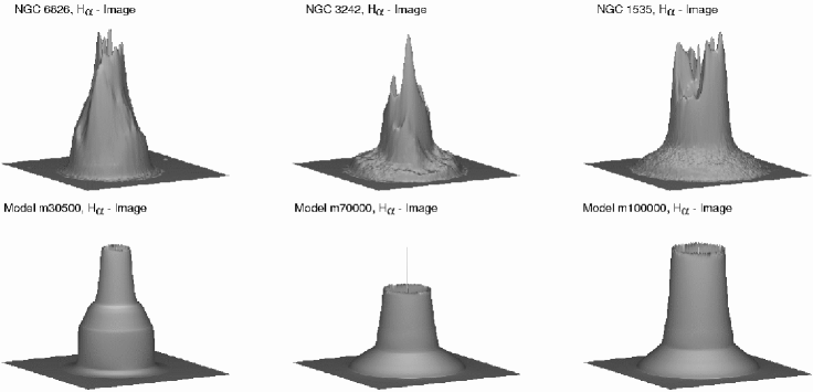
Figure 1: Top: normalized 3D representations of the H$\alpha$ images of NGC~6826 (left), NGC~3242 (middle), and NGC~1535 (right). The images are from an unpublished catalogue compiled by Bässgen (priv. communication). Bottom: corresponding H$\alpha$ surface brightness profiles of optically thin models selected from the hydrodynamic sequence No. 6 listed in Table 2. Post-AGB ages increase from left to right. The normalizations of the models are adjusted as to match those of the observed objects.

The success of these detailed radiation-hydrodynamics simulations in describing planetary nebulae is illustrated in Fig. 1 where we compare the H$\alpha$ brightness distributions of 3 PNe with well-developed double-shell structures with the model predictions. The models are selected from sequence No. 6 of Table 2 which started with an initial envelope computed by means of two-component radiation-hydrodynamics simulations along the upper AGB (Type C, see Steffen et al. 1998, for more details).

Although the models are spherically symmetric, they represent the observed general structures as indicated by the H$\alpha$ brightness distribution astoundingly well: the brightness ratio between both shells, i.e. ‘rim’ and ‘shell’, is well matched, and also the linear brightness slope of faint ‘shells’, typical for many nebulae, is reproduced. Such a linear radial brightness profile of the ‘shell’ develops if the radial density gradient of the circumstellar envelope steepens with distance from the star, indicative of increasing mass loss towards the end of the AGB evolution (Steffen et al. 1998; Schönberner et al. 2005a). More comparisons between observed structures of planetary nebulae and the predictions of our radiation-hydrodynamics simulations can be found in Steffen & Schönberner (2006).

2.2 General behaviour of our nebular models

For a better appreciation of the differences between our hydrodynamical models and those developed by Marigo et al. (2001) it appears to be useful to give a brief description of the basic principles of the formation and evolution of planetary nebulae as they follow from recent realistic hydrodynamics simulations. In Paper I we introduced several phases of the PN evolution according to the main physical processes acting on the whole system. We briefly repeat them here, using the models of sequence No. 6 for illustration.

Neglecting the proto-planetary-nebula phase which is of no interest here, the first important phase, the ionisation phase, begins when the intense flux of ionising photons from the central star starts to ionise and to heat the inner parts of the AGB wind envelope. The large thermal pressure of the ionised gas determines shape and expansion of the newly created PN. The ionisation front is of type D and trapped by a strong, nearly isothermal shock (see Fig. 2, top panel).

The bottom panel of the figure depicts the ionisation structure of oxygen, which is of particular interest for the present study. The degree of ionisation is still rather moderate: neutral in the undisturbed AGB wind, singly ionised preferently in the outer and doubly ionised in the inner parts of the ionised shell.

The ionisation phase finishes if the ionisation front passes the shock and propagates quickly through the still undisturbed AGB matter (R-type ionisation front). The PN is then optically thin for ionising radiation and said to be density bounded. Figure 3 depicts a moment well after the thick/thin transition. The outer boundary of the PN is now the shock front enclosing the ‘shell’, and not the ionisation front which has already left the computational domain. The main ionisation stage of oxygen is O⁺² throughout the shell and the halo, except in the inner part of the rim where we have already O⁺³. Helium is also doubly ionised in this inner region, and the extra heat deposited by the ionisation of He⁺ drives a weak shock (at $r=1.3\cdot 10^{17}$ cm in Fig. 3, top panel).

Figure 2: Top: radial profiles of heavy-particle density (thick), electron density (dotted), and velocity (thin) of an optically thick model selected from sequence No. 6. The stellar parameters of the 0.605 M_☉ central star are $T_{\mathrm{eff}}=40\,245$ K and $L=6240$ L_☉, with a post-AGB age $t=2478$ yr. Bottom: ionisation fractions of neutral (dotted), singly ionised (dashed), and doubly ionised oxygen (dash-dotted). The ionisation fractions within the shocked central-star wind domain ($r\leq 0.5\cdot 10^{17}$ cm), though computed, are not shown for clarity.

Figure 3: Same as in Fig. 2, but for an optically thin model with well developed rim and shell structures. The stellar parameters are $T_{\mathrm{eff}}=79\,708$ K and $L=5797$ L_☉, with a post-AGB age $t=4241$ yr. The dash-triply dotted line indicates triply ionised oxygen.

The model PN is now in the compression phase in which the high pressure of the shock-heated central-star wind accelerates and compresses the inner parts of the shell into the so-called ‘rim’. The rim becomes the dominant structure of a PN, and the objects displayed in Fig. 1 are in this stage. The compression phase is terminated when the wind power declines because the central star is approaching its maximum effective temperature and fades towards a white-dwarf configuration.

Figure 4: Same as in Fig. 2, but for an optically thin model at the end of the compression phase close to maximum stellar temperature. The stellar parameters are $T_{\mathrm{eff}}=156\,662$ K and $L=2075$ L_☉, with a post-AGB age $t=7124$ yr.

Figure 4 shows a model very close to maximum stellar temperature at the end of the compression phase. At the large effective temperature well above 100 000 K a significant fraction of oxygen is now triply ionised. There exists, however, still some singly ionised oxygen close to the outer edge of the shell.

During the whole compression phase the leading edge of the shell continues to propagate supersonically into the AGB wind with a (relative) speed ruled only by the thermal properties of the gas and the radial density profile of the AGB wind (Franco et al. 1990; Chevalier 1997; Shu et al. 2002; Schönberner et al. 2005a). The expansion of the shell is not at all influenced by the wind interaction responsible for the formation of the rim. Usually, the shell expands faster than the rim (see Paper II, Fig. 12 therein).

The final fading of the central star causes recombination in the outer parts of the PN provided the nebular densities are sufficiently large, and/or the luminosity declines very rapidly. Recombination turns eventually into re-ionisation after the fading of the central star has slowed down and the nebular density becomes sufficiently low due to the continued expansion.

Figure 5: Same as in Fig. 2, but for a model after the end of recombination and at the beginning of re-ionisation. The stellar parameters are $T_{\mathrm{eff}}=122\,269$ K and $L=249$ L_☉, with a post-AGB age $t=9557$ yr.

The model shown in Fig. 5 illustrates the situation after the end of the recombination and at the beginning of the re-ionisation stage. The shell is mainly neutral, although not completely, and forms for a while a recombination halo (Corradi et al. 2000). The rim which remained fully ionised to a large extent continues to expand and will eventually swallow the shell material because the shell’s shock is slowed down during recombination. The ionisation is highly stratified (bottom) and reflects the physical situation given by a central star of low luminosity but still very high effective temperature: mainly O⁰ in the shell, but the degree of ionisation increases inwards over O⁺ until O⁺³ at the inner rim.

These main evolutionary stages as described here may not always occur, or they may even occur at the same time. For instance, a PN around a low-mass, slowly evolving central star will not recombine at all. On the other hand, a PN around a massive, very quickly evolving central star may not become optically thin. In this case the ionisation front remains always of type D, i.e. trapped by the outer shock, and we have ionisation and compression at the same time. However, the double shell configuration is very robust and develops also in these cases.

This discussion shows that the formation of typical PN structures is quite complex even in the spherical approximation. Two processes are relevant, viz. heating by ionisation and compression by wind interaction. Their relative importance will depend on the metallicity, i.e. on the content of coolants. For instance, at lower metallicities than we have used here we expect (i) less dense rims simply because the central-star wind power is most likely lower, and (ii) higher expansion rates of the shell because the temperature, and sound speed, is larger.

A completely different situation is encountered in systems with a Wolf-Rayet central star. The virtually hydrogen-free wind from such a star is up to two orders-of-magnitude more intense compared with objects of normal surface abundances (cf. Leuenhagen et al. 1996). Consequently, wind interaction will always be dominant for shaping a PN around a Wolf-Rayet central star, independently of the general metallicity. Since origin and evolution of hydrogen-poor central stars is not known, nebular models around them can not be computed to date. The sequences listed in Table 2 und used here have exclusively central-star models with normal surface composition burning hydrogen to provide their luminosity.

3 Comparison with the Marigo et al. models

As already mentioned in the Introduction, the approach of Marigo et al. (2001) to compute the evolution PNe analytically goes back to methods developed by Volk & Kwok (1985). Marigo et al. introduced several improvements, the most important one being the approximate consideration of radiative processes, viz. heating by ionisation and cooling by line emissions. However, an analytical treatment of the dynamics of photoionisation oversimplifies the problem and has severe consequences.

For instance, the basic nebular structures of the Marigo et al. models are shells of constant density which are partially or fully ionised. They are in full contrast to real objects which have complicated density and velocity profiles and which can only be approximated by hydrodynamical models (cf. Figs. 2 till 5). In a typical double-shell PN most of the nebular mass ($\ga\!80\,\%$) is contained in a shell of rather low density and expands independently of the properties of the central-star wind, as explained in the previous section. Only the small fraction of nebular matter contained in the rim is ruled by wind interaction.

The density structure of a PN, however, is important for the ionisation balance since local photoionisation rates are proportional to density, recombination rates, however, proportional to density squared. On one hand, the ionisation front may be kept trapped for quite a while during the early evolution when the nebular densities are still large (D-type front), resulting in a delay of the thick/thin transition. On the other hand an extended, low density shell is less prone to recombination than a Strömgren sphere of the same mass but with larger, constant density. The question of the nebula’s optical thickness to ionising radiation, however, is crucial for the emission-line luminosities and for the interpretation of the luminosity function (see Méndez et al. 1993; Méndez & Soffner 1997).

The influence of the different treatment of nebular shells becomes evident by a direct comparison between the properties of the hydrodynamical models with those of Marigo et al. (2004). For this purpose, we selected our sequence No. 6a together with the sequence No. 4 of Marigo et al. (2001, Table 2 and Fig. 9 therein). Both simulations are based on central stars with very similar masses (0.595 vs. 0.5989 M_☉), and also their final AGB mass-loss rates are about the same, $\approx\!10^{-4}$ M_☉ yr^-1. Both sequences may be considered as typical representatives for the planetary nebula evolution.

The Marigo model becomes optically thin in the Lyman continuum very early, at about 25 000 K. It remains optically thin until the central star fades below 1000 L_☉ along the cooling part of the track where the shell recombines (Fig. 10 in Marigo et al. 2001). In our model, the ionisation front remains trapped behind a strong shock until the central star becomes as hot as $T_{\mathrm{eff}}\simeq 47\,000$ K.

A direct observational test about the quality of PN simulations is possible by considering the (relative) geometrical thickness of the whole nebular structure. We define the total relative thickness of a PN as $\delta R=(R_{\mathrm{out}}-R_{\mathrm{cd}})/R_{\mathrm{out}},$ with $R_{\mathrm{out}}$ and $R_{\mathrm{cd}}$ being the radial positions of the outer nebular boundary and of the contact surface, resp. The nebular boundary is either defined by the ionisation front (optically thick case) or by the shell’s shock for density bounded, optically thin models. During the recombination phase, the position of the recombination/ionisation front can not be determined precisely, nor is the recombination complete (see Fig. 5). We thus defined $R_{\mathrm{out}}$ in general by the radial position where 99 % of the total H$\beta$ line emission from the nebular model is included.

The difference between $R_{\mathrm{out}}$ as defined above and the position of the shock, $R_{\mathrm{shock}}$, is negligible as long as the ionisation is complete. During recombination the outer parts of the shell may become faint to such an extent that $R_{\mathrm{out}}$ gets smaller than $R_{\mathrm{shock}}$. For example, the model shown in Fig. 5 is at the end of its recombination phase, and we have $R_{\mathrm{out}}=8.8\cdot 10^{17}$ cm and $R_{\mathrm{shock}}=9.6\cdot 10^{17}$ cm.

Instead of plotting $\delta R$ vs. time or $R$, we used the stellar temperature as a distance-independent proxy for the post-AGB age because formation and evolution of the nebular structure is ruled by the radiation field and the wind from the central star, both of which depend directly or indirectly on the effective temperature. The choice of the stellar temperature has the advantage that its range depends only modestly on stellar mass, much in contrast to the evolutionary time scale.

The variation of $\delta R$ with stellar effective temperature for the hydrodynamical model sequences used here (see Table 2) and for the Marigo sequence selected above is displayed in Fig. 6. At low effective temperatures, the differences between the Marigo and our models are quite small, i.e. $\delta R$ increases rapidly to about 0.6. Then our models remain rather extended for the whole transition across the Hertzsprung-Russell diagram, while $\delta R$ of the Marigo models decreases steadily from its maximum value of $\approx\!0.7$ to about only 0.2. At this low value the model becomes optically thick by recombination (cf. Fig. 9 in Marigo et al. 2001).

Once the star has passed its maximum effective temperature, the outer regions of the hydrodynamical models may recombine more or less strong, leading to a rapid reduction of $\delta R$ to values as small as $\simeq\!0.05$ for the above adopted 99% criterium for the determination of $R_{\mathrm{out}}$. Re-ionisation finally brings $\delta R$ up again.

The different model predictions concerning the geometrical structure of PNe can easily be checked against observations. However, instead of using data from the literature, we preferred to remeasure the thicknesses of a number of well-known PNe whose (monochromatic) images were at our disposal, viz. the objects discussed in Paper II and Paper III. While the outer edge of a PN, i.e. the location of the shell’s shock, is easy to measure, the position of the inner edge, given by the contact surface, is not so obvious. However, the surface brightness of nebular models reveal that the peak brightness of the rim in [O iii] (or in H$\alpha$) indicates the radial position of the contact surface. Guided by the models, we determined the relative thicknesses, $\delta R$, along the semi-minor axes by means of surface brightness plots derived from the monochromatic images and present the results in Table 3.

Figure 6: Relative geometrical thickness, $\delta R=(R_{\mathrm{out}}-R_{\mathrm{cd}})/R_{\mathrm{out}}$, of PNe predicted by the different hydrodynamical sequences from Table 2, and by a sequence of Marigo et al. (2001, Figs. 9 & 11 therein) vs. the effective temperatures of the respective central stars, where the temperatures are used as proxies for the post-AGB ages. The total times shown are 3 000 yr for sequence No. 10, 10 000 yr for No. 8, about 15 000 yr for the Marigo et al. sequence, and about 20 000 yr for the sequences Nos. 4, 6, and 6a. For comparison, the measured $\delta R$’s of the PNe from Table 3 are plotted, too (filled circles).

Table 3: Relative geometrical thicknesses, $\delta R=(R_{\mathrm{out}}-R_{\mathrm{cd}})/R_{\mathrm{out}}$, measured along the semi-minor axis for a sample of well-observed PNe. The images used were either retrieved from the HST data archive, or they were taken with ground-based telecopes .

Object	$T_{\mathrm{eff}}$ [K]	$\delta R$	Comments
IC 418	36 000	0.78	HST
IC 2448	65 000	0.65	HST
NGC 1535	70 000	0.64	Ground based
NGC 2022	100 000	0.55	Ground based
NGC 2610	100 000	0.49	Ground based
NGC 3242	75 000	0.61	HST
NGC 6578	67 000	0.61	HST
NGC 6826	50 000	0.72	HST
NGC 6884	87 000	0.64	HST
NGC 7027	$\simeq\!200\,000$	0.41	HST ⋆
NGC 7662	100 000	0.64	HST
My 60	105 000	0.70	Ground based

^⋆ Semi-major axis (cf. Paper III).

Our measured values listed in Table 3 cluster around $\delta\approx 0.6$ and are thus substantially larger than claimed by Zhang & Kwok (1998) who found typical values between 0.3 and 0.6. However, these authors considered only the bright nebular structures, viz. the rim in the cases of double shell PNe, ignoring the fact that the major part of the nebular mass is contained in the shell. Using the data of Zhang & Kwok (1998) we found an average value of only $\delta R\simeq 0.40$ for the 7 objects in common. Inclusion of the shells would increase their (relative) thicknesses to our values.

Figure 6 indicates that the relative thickness of PNe, once established by photoionisation during the early evolution, decreases only slightly during the further evolution across the Hertzsprung-Russell diagram, if at all. Our hydrodynamical models are in excellent agreement with the observations, contrary to the presented sequence of Marigo et al. (2001) whose models become geometrically too thin during the course of their evolution. The reason for this difference is the behaviour of the propagation velocities of the outer shock and the contact discontinuity in the hydrodynamic approach: both are accelerated such that the relative distance between them does not change much. For a detailed discussion of the expansion properties of hydrodynamical models see Paper II and Paper III. We emphasize that our sequences shown in Fig. 6 span a range of final masses between 0.57 and 0.7 M_☉ with the corresponding spread of initial masses. Also, all the observed objects shown in the figure are on the high-luminosity part of their evolution to the white-dwarf domain.

As can be seen from Fig. 17 in Marigo et al. (2001), all their models behave like the one shown in Fig. 6, i.e. $\delta R$ attains very low values around or even below 0.2 in the hot region of the Hertzsprung-Russell diagram where the evolution is slowed down shortly before the maximum effective temperature of the central star is reached. Yet the Zhang & Kwok (1998) sample contains only very few objects with $\delta R\la 0.3$. Their whole sample can only be reproduced by a superposition of sequences with different evolutionary time scales, a fact that does not seem to be very likely. We iterate that the real thickness of most objects from the Zhang & Kwok sample shown in Fig. 17 of Marigo et al. (2001) is certainly larger, making it even more difficult to accept such a comparison as support for the Marigo et al. models.

Marigo et al. (2001) conducted several other tests to verify the usefulness of their models. Unfortunately, these tests suffer from inaccurate and inhomogeneous data and/or only poorly known distances. This concerns diagrams like ionised mass vs. nebular size and electron density vs. nebular size. Our sequences passed these tests equally well.

A more specific comment on the use of expansion velocity–radius diagrams appears to be in order. It has been shown by means of hydrodynamical simulations that the term ‘expansion velocity’ has to be treated with utmost care (cf. ; , ). The expansion measured by Doppler-split lines refers to a typical flow speed within the nebular structure, while the real nebular expansion is given by the propagation of the shell’s shock front. A diagram like the one shown in Fig. 21 of Marigo et al. (2001) where (observed) flow velocities are compared with boundary velocities or averages of them is certainly problematic.

An additional uncertainty is being introduced by comparing model velocities with the Weinberger (1989) compilation of expansion velocities. This data set is extremely inhomogeneous, and the entries refer mainly to the bright parts of the PNe which dominate the line emission and which are by no means representative for the real nebular expansion (cf. Gesicki et al. 1996). In Paper II we demonstrated that, once the initial conditions for the modelling are properly chosen and the expansion of objects correctly measured, hydrodynamical models give a reasonable description of the expansion properties of those planetary nebulae which do not differ too much from a spherical/elliptical shape.

A distance independent observational test of relevance is the one on the typical structures of PNe conducted above. Real PNe are obviously not very compressed, and their outer parts do not recombine totally during the later phases of their evolution. The reason for the larger extent of real objects (and of our models) is the generation of a shock wave by photoionisation whose propagation is ruled by the electron temperature and the density gradient of the circumstellar matter and cannot be derived by applying energy and momentum balances based on a wind interaction scenario. It is the different physical description that obviously leads to the structural differences between our hydrodynamical and the Marigo et al. (2001) models.

Based on all these facts we believe that our hydrodynamical models are better representatives of real planetary nebulae than the Marigo et al. models. Further support for this statement is presented in Sect. 4.5.

Figure 7: Number of ionising photons emitted per second by a 0.605 M_☉ post-AGB model as a function of age (top) and effective temperature (bottom), under the assumption that the stellar photosphere radiates as a black body. Plotted are the relations for hydrogen ($\lambda<912$ Å), neutral helium ($\lambda<504$ Å) and singly ionised helium ($\lambda<228$ Å), and for singly ionised oxygen ($\lambda<353$ Å).

4 Evolution of emission lines

With our hydrodynamical models we have the means to investigate in a more realistic way how the line emission depends on the central star’s luminosity and effective temperature, and also on the nebula’s optical depth, as the whole system evolves across the Hertzsprung-Russell diagram. Previous attempts to follow the line emission along an evolutionary track are based on purely kinematic models with simple geometries, constant densities, and ionisation equilibrium (e.g. Vilkoviskii et al. 1983; Stasińska 1989).

The line emission from a PN is, as is well known, determined by the ionising photon flux from the central star and the optical depth of the nebular shell. Figure 7 illustrates the run of the number of ionising photons emitted per second with age (top) and effective temperature (bottom) for the two 0.605 M_☉ sequences (Nos. 4 and 6). Note that these total photon numbers depend not only on the effective temperature but also on the stellar radius, which explains the large variations with time or temperature.

Figure 8: Changes of stellar (thick dashed) and nebular line luminosities (solid lines), $L$, and of the numbers of ionising photons emitted per second, $N$ (long dashed), with post-AGB age for a 0.605 M_☉ central-star model combined with two different envelope models according to the sequences No. 4 (thick line) which never becomes optically thin and No. 6 (thin line) which becomes thin to ionising photons during the course of evolution. Top: evolution of $L_{\star}$, $L({\rm H}\beta)$, and $N_{<912}$ (right ordinate). Bottom: the same but for $L_{\star}$, $L(5007)$, and $N_{<353}$ (right ordinate).

The influence of the optical depth is highlightened in Fig. 8 which shows the evolution of the nebular H$\beta$ and [O iii] line emissions with time for the 0.605 M_☉ central star model coupled to two different nebular models (sequences Nos. 4 and 6). In the top panel the number of photons emitted per second below 912 Å, $N_{<912}$, is compared with the H$\beta$ luminosity, whilst in the bottom panel the relevant quantities for [O iii] are given: $N_{<353}$ and $L(5007)$, respectively. For comparison, the stellar luminosity is also displayed in both panels.

For the optically-thick case of sequence No. 4, the line luminosities follow closely the number of ionising photons emitted per second, as expected from theory. While for hydrogen the maxima of the H$\beta$ emission and $N_{<912}$ occur at the same time (and at the same stellar temperature), the [O iii] line emission peaks before $N_{<353}$. The reason is that, at the high stellar temperatures involved, the prevailing ionisation stage shifts slowly from O⁺² to O⁺³ (see Sect. 4.3 for a more thorough discussion).

As long as the models of sequence No. 6 are optically thick for ionising photons, their line emission is almost identical to that of sequence No. 4. When the models become thin, their line emission drops below the value of an corresponding optically thick model: the ionised masses become smaller, and the nebula is said to be ‘density bounded’. Later on, after about 7 000 years of post-AGB evolution, the ionisation drops in line with the decreasing central-star luminosity, and the outer parts of the models recombine to a large extent. Consequently the nebular shell becomes able to absorb nearly all ionising photons again, and both sequences show virtually the same line luminosity for some time.

The small differences between both sequences, after recombination has started, have several causes. Firstly, recombination is not complete, i.e. the outer regions of the models of sequence No. 6 do not become fully neutral (in hydrogen). Secondly, we have to consider non-equilibrium effects due to the rapid fading of the stellar luminosity. Because the two sequences shown in Fig. 8 have different densities, recombination occurs with different time scales. In particular, the models of sequence No. 6 are less dense than the corresponding ones of sequence No. 4, and consequently they recombine more slowly. Thirdly, because of their expansion the models of sequence No. 6 begin to reionise, reducing thereby their optical depth to such an extent that their line emission falls again below that of sequence No. 4 (cf. $L({\rm H}\beta$) for $t\ga 10\,000$ yr). At this particular evolutionary phase where the stellar luminosity and temperature changes only very little, the degree of ionisation is exclusively controlled by expansion.

Oxygen recombines faster than hydrogen, thus its ionisation state can more easily keep pace with rapidly changing ionisation rates. Indeed, after recombination the [O iii] luminosities of both sequences are virtually the same (see Fig. 8, bottom). But beyond $t\approx 15\,000\,{\rm yr}$ the models of sequence No. 6 become optically thin again by re-ionisation and their [O iii] emission falls below that of sequence No. 4.

Since one has to consider that most observed PNe are optically thin to different degrees, one has to take into account the thick/thin transition for any realistic modelling of the PNLF. Using our hydrodynamical simulations we will discuss in Sects. 4.1 to 4.3 in more detail how the line emission of hydrogen, helium, and oxygen depends on the different model properties.

4.1 The H$\beta$ luminosity

We begin with a discussion of the H$\beta$ luminosity displayed in Fig. 9 for four different model sequences selected from Table 2. The models of the sequences Nos. 4 and 10 remain always optically thick while those of sequences Nos. 6 and 6a, both with the same Type C initial envelope, become optically thin for Lyman continuum photons at stellar effective temperatures between 45 000 and 60 000 K.

Figure 9: $L({\rm H}\beta)/L_{\sun}$ (top) and $L({\rm H}\beta)/L_{\star}$ (bottom) vs. stellar effective temperatures for four model sequences from Table 2 with 0.696 M_☉ (No. 10), 0.605 M_☉ (No. 4), 0.605 M_☉ (No. 6), and 0.595 M_☉ (No. 6a). The circles mark the transition from the optically thick to the optically thin stage (Nos. 6 and 6a only, see text for details). The endpoints of the tracks correspond to post-AGB ages of 20 000 years (Nos. 4, 6, 6a) and 3 000 years (No. 10), respectively.

It is known from photoionisation models that the transition from the optically thick to the thin stage is not well defined. The ionisation front is not sharp in a mathematical sense, and the model’s optical depth depends also on the wavelength considered. Even if a model is still optically thick, high-energy photons with their lower absorption probability may well escape. A rather illuminating discussion of the optical depth problem in gaseous nebulae has been presented by Gruenwald & Viegas (2000). In the present work we define the optically thick/thin transition in a rather pragmatic way as the moment when the H i/ii ionisation front passes the leading shock. This moment is marked by circles in Fig. 9.

Figure 9 (top panel) demonstrates that the two optically thick sequences (Nos. 4 and 10) reach maximum H$\beta$ luminosities at a stellar effective temperature of about 65 000 K, exactly where also $N_{<912}$ peaks due to the evolution of the stellar radius with effective temperature as the central star evolves across the HR diagram (see Fig. 7).

In the bottom panel of Fig. 9 the evolutionary influence of the central star is taken out, and one sees immediately that the maximum efficiency of converting Lyman photons into H$\beta$ photons occurs at a stellar temperature of about 70 000 K. At fixed stellar luminosity, $N_{<912}$ reaches a maximum at about 70 000 K because of the following reason: In general, the total number of stellar photons emitted per second, $N_{\rm total}$, decreases with increasing effective temperature because the fraction of high-energy photons becomes larger. Now, at lower temperatures, $N_{<912}$ increases very rapidly with temperature, and so does the H$\beta$ luminosity. At very large temperatures, however, $N_{<912}$ approaches $N_{\rm total}$ and must finally decrease with temperature like $N_{\rm total}$.

The existence of a maximum H$\beta$ luminosity (or flux) at intermediate stellar temperatures has already been shown, but not explained, by Dopita et al. (1992) using a series of optically thick photoionisation models. The optimal efficiency of converting stellar luminosity into H$\beta$ line luminosity is about 1 % (bottom panel of Fig. 9). This value, of course, will not be reached if the PN shell becomes optically thin, as is the case for the sequences Nos. 6 and 6a.

Once the central star has reached the hottest point of its evolution, it may shrink so rapidly towards white dwarf dimensions that the outer, less dense parts of the nebular shell may deviate from ionisation equilibrium for some time, as already mentioned in the previous section. For instance, once the star has passed its maximum effective temperature, it fades with time scales, $L_{\star}/\dot{L_{\star}}$, depending on its mass: $\simeq$ 400 yr for 0.595 M_☉, $\simeq$ 200 yr for 0.605 M_☉, and only about 20 yr in the case of 0.696 M_☉.

Non-equilibrium phases are best seen in the bottom panel of Fig. 9. One sees clearly that the H$\beta$ luminosity of all models, albeit to different extents, do not follow the stellar luminosity decline after maximum stellar temperature. The extended ‘loops’ indicate that the recombination rates considerably exceed the ionisation rates during the rapid stellar luminosity decline. They are very pronounced for the sequences Nos. 6 and 6a, but still visible for the sequences Nos. 4 and 10 despite of their rather dense, optically thick nebular shells. Recombination exceeds ionisation for about 1500 years for the 0.605 M_☉ case (No. 4), but only about 40 years for 0.696 M_☉ (No. 6). Except for the 0.595 M_☉ models, the H$\beta$ luminosity exceeds then even the limit given by equilibrium ionisation. The latter is finally reached again after the evolution is slowing down while the central star is settling onto the white-dwarf sequence.

Our models show that non-equilibrium ionisation of hydrogen may last for quite a substantial fraction of the total PN lifetime (up to 10 %). Considering the fact that heavier ions recombine much faster than hydrogen, the conclusion is that line strengths measured relative to that of hydrogen become smaller during the recombination phase, leading consequently to erroneous results when standard plasma analysis methods are applied.

During the non-equilibrium recombination phase, the efficiency of converting stellar photons into H$\beta$ photons temporarily exceed the maximum value typical for equilibrium conditions (Fig. 9, bottom). This may also hold for optically thin cases (cf. sequence No. 6). The absolute H$\beta$ luminosities, however, remain always well below the maximum gained earlier at intermediate stellar temperatures (top panel of Fig. 9). We conclude thus that the maximum H$\beta$ luminosity of a PN is achieved either at $T_{\mathrm{eff}}\simeq 65\,000$ K for the optically thick case, or at lower temperatures if the nebular envelope becomes optically thin earlier.

Figure 10: $L({4686})/L_{\sun}$ (top) and $L({4686})/L_{\star}$ (bottom) vs. stellar effective temperatures for the same sequences as in Fig. 9.

4.2 The He ii luminosity

Although the helium lines are of no interest for luminosity functions, we present here, for completeness, the properties of the He ii 4686 Å emission as they follow from our simulations (Fig. 10). By comparing with Fig. 9 we see that the He ii emission peaks at effective temperatures well beyond 100 000 K, at a position that depends on the evolutionary properties of the central star, i.e. the larger its mass, the larger will be the peak temperature. Only the 0.595 M_☉ models (No. 6a) become optically thin for photons with $\lambda<228$ Å once the temperature of the central star exceeds 120 000 K.

The maximum efficiency in converting stellar radiation into He ii 4686 Å line emission is only reached beyond 250 000 K and is about 0.3 % (Fig. 10, bottom panel). Because most central stars will not reach such high temperatures, and also because some nebulae will become optically thin for photons below 228 Å (sequence No. 6a), the maximum absolute 4686 Å emission is expected to occur at stellar temperatures between 100 000 and 150 000 K (top panel).

Non-equilibrium effects are expected to be modest because He⁺² recombines much faster than H⁺. Indeed, we see only small deviations from the equilibrium curves for the sequences Nos. 6, 6a, and also a very small ‘loop’ for sequence No. 4, but not for the very dense 0.696 M_☉ models of sequence No. 10 (Fig. 10, bottom panel).

Figure 11: $L(5007)/L_{\sun}$ (top) and $L(5007)/L_{\star}$ (bottom) vs. stellar effective temperatures for the same sequences as in Fig. 9. The dotted horizontal line indicates $L(5007)=620\leavevmode\nobreak\ L_{\sun}$. The circles indicate where the models become optically thin for Lyman continuum photons (Nos. 6 and 6a only).

4.3 The [O iii] 5007 Å luminosity

Understanding the behaviour of the [O iii] 5007 Å emission from the nebular shell as the central star evolves across the HR diagram is the key for any understanding of observed PNLFs. The interpretation of this emission is more difficult since it depends strongly on the ionisation structure of oxygen which is a strong function of the evolutionary state (see Figs. 2–5).

The run of the [O iii] 5007 Å luminosity along different evolutionary tracks is displayed in Fig. 11. The absolute [O iii] luminosity peaks already between 95 000 and 100 000 K (top panel), while the efficiency of converting stellar luminosity into 5007 Å line radiation reaches a maximum close to 110 000 K (bottom panel), although $N_{<353}/N_{\rm total}$ peaks at about 180 000 K, for the same reasons as discussed in Sect. 4.1. The maximum conversion efficiency is about 10 % for the composition used here (cf. Dopita et al. 1992), but does not change much until the stellar luminosity begins to fade. The more luminous 0.696 M_☉ sequence shows a slightly larger conversion efficiency simply because of its somewhat larger electron temperature.

The position of the maximum of the conversion efficiency and the relatively flat run of the latter with stellar effective temperature is the result of two competing effects: On one hand, the ionisation of oxygen shifts from O⁺² to O⁺³ with increasing stellar temperature (see Figs. 3 and 4). On the other hand, the electron temperature rises steadily until the maximum stellar temperature is reached and compensates partly for the (relative) decrease of the emitting mass. The electron temperature range is from 8 000 to 12 000 K for the 0.605 M_☉ case (sequence No. 4) and from 9 000 to 14 000 K for the 0.696 M_☉ case (sequence No. 10).

The models of the sequences Nos. 6 and 6a become optically thin for O⁺ ionising photons at 55 000 and 65 000 K, respectively, which means after they became thin for Lyman continuum photons (circles). It is important to note that at this particular thick/thin transition the 5007 Å luminosity attains its (absolute) maximum (top panel of Fig. 11).

Because ionised oxygen recombines also much faster than H⁺, we do not expect important non-equilibrium effects for the [O iii] emission. Rather, the large ‘loops’ apparent in Fig. 11 for the optically thin sequences are mainly the consequence of the changing ionisation structure of oxygen. As already mentioned above, during the hottest, high-luminosity part of the stellar track the ionisation of oxygen is partly shifted towards the third stage (Fig. 4). When the stellar luminosity begins to drop, O⁺² becomes temporarily the main ionisation stage, leading for a brief moment to a local maximum of the O⁺² mass and of $L(5007)/L_{\star}$ (cf. Fig. 11, bottom). With further decreasing stellar luminosity, recombination continues from O⁺² to O⁺, and $L(5007)$ drops very rapidly.

Due to the significant fraction of O⁺ expected in nebular shells surrounding low-luminosity central stars (cf. Fig. 5), the UV photon conversion efficiency drops considerably below its maximum value of $\approx 0.1$, as is seen for sequences Nos. 6 and 10 in Fig. 11 (bottom). This is different from the hydrogen case where the conversion efficiency is, in the optically thick case, only a function of the stellar effective temperature provided ionisation is in equilibrium (cf. Figs. 9 and 11). The [O iii] luminosities of the models from the sequences Nos. 6 and 6a lie during their recombination ‘loops’ temporarily somewhat above the luminosities of the models from sequence No. 4, indicating a small imbalance between recombination and ionisation during the rapid luminosity decline of their central stars.

The luminosity evolution of our hydrodynamical models as shown in the upper panel of Fig. 11 differs completely from the predictions of Marigo et al. (2004). According to their nebular models, which become optically thin very early, the 5007 Å line luminosity increases steadily during the crossing of the Hertzsprung-Russell diagram. Shortly before the turning point is reached, the models become optically thick due to the reduced supply of ionising photons, and this thin/thick transition constitutes the moment of maximum [O iii] line emission since afterwards the emission always decreases for the same reasons as in the case of H$\beta$ (see Fig. 10 in Marigo et al. 2004): the stellar luminosity decreases, and the UV photon conversion efficiency is below its maximum as well.

In conclusion we state that, for the metallicity chosen here, the maximum [O iii] line emission of a PN occurs at $T_{\mathrm{eff}}\simeq 95\,000\dots 100\,000$ K for optically thick configurations, or at lower temperatures if the PN becomes optically thin.

Figure 12: Correlations of line ratios between H$\beta$, He ii 4686 Å, and [O iii] 5007 Å, as predicted by our models and as observed for highly excited PNe (circles). The evolution proceeds from the right lower corner with low 4686/H$\beta$ towards large 4686/H$\beta$ values at maximum stellar temperatures. The inset provides an enlarged view of the highest-excitation domain. The circles represent LMC planetaries selected from Meatheringham & Dopita (1991a, b).

4.4 Line ratios

Before continuing we will discuss line ratios between important emission lines i.e. between H$\beta$, He ii 4686 Å, and [O iii] 5007 Å. The relative strengths of these lines reflect the ionisation structure of the nebula, determined mainly by the intensity and spectral energy distribution of the stellar radiation field and the optical depth of the nebular shell. For instance, we see from the theoretical predictions in Fig. 12 that for any given 4686/H$\beta$ line ratio, the corresponding 5007/4686 ratio becomes smaller with decreasing central-star mass: For more slowly evolving central stars the nebular shell becomes more diluted with increased ionisation, leading to smaller 5007/4686 line ratios.

We compare our models with a sample of LMC PNe taken from Meatheringham & Dopita (1991a, b). This sample has the advantage that it is homogeneous and that the line fluxes are representative for the whole object. We see from Fig. 12 that the anti-correlation between 4686/H$\beta$ and 5007/4686 shown by the Magellanic Cloud PNe sample seems very well be explained by our hydrodynamic simulations within a central-star mass range of 0.59…0.63 M_☉. Note that the observed very low 5007/4686 values ($\simeq 10$) are only reached by those sequences with optically thin models (sequences Nos. 6, 6a, and 22).

We caution, however, that the anti-correlation shown in Fig. 12 is not sensitive to the overall structure of the models: Marigo et al. (2001, 2004) demonstrated that their models are also able to match the observed anti-correlation.

4.5 Nebular excitation

A very useful tool to classify the line emission of a PN and to determine its evolutionary stage is the excitation, expressed by suitable emission line ratios. We follow here the definition introduced by Dopita et al. (1992) and write for the excitation parameter $E$:

$$E=0.45\,\left[L(5007)/L({\rm H}\beta)\right],\ \ \ \ \hskip 54.06006pt0.0<E<5.0\,,$$

$$E=5.54\,\left[L(4686)/L({\rm H}\beta)+0.78\right],\ \hskip 28.45274pt5.0\leq E<12.0\,.$$ (2)

Using this definition, we computed $E$ for our model sequences and plotted the result against the absolute H$\beta$ and 5007 Å magnitudes (Fig. 13). A similar diagram, although based on pure photoionisation models, has been introduced and used by Dopita & Meatheringham (1990) to study the evolution of Magellanic Cloud PNe.

Figure 13: Nebular excitation parameter, $E$, vs. absolute H$\beta$ (top) and 5007 Å magnitudes (bottom) for different hydrodynamical sequences with 0.696 M_☉ (No. 10), 0.605 M_☉ (Nos. 4 and 6), 0.595 M_☉ (No. 6a), and 0.565 M_☉ (No. 22). Absolute magnitudes are based on Eq. (1). The small gaps between $E\!\approx 4$–$5$ for the sequences Nos. 6a and 22 are artifacts due to the definition of $E$ (see text). The open circles indicate again the thick/thin transition of the nebular models (that of the 0.565 M_☉ sequence is outside the plotted range). Data of galactic PNe with spectroscopically determined distances are shown for comparison (Méndez et al. 1993, dots). The ‘circled’ dot belongs to NGC~7293, the two ‘squared’ dots to the high-excitation PNe NGC~1360 and NGC~4361. The filled triangle marks the position of NGC~7027.

The evolution in Fig. 13 proceeds from low to high excitation, viz. the excitation increases generally with increasing stellar effective temperature. The maximum value of $E$ is reached at the highest possible stellar temperature because the $4686/{\rm H\beta}$ line ratio becomes largest there. The actual value depends on the stellar mass, i.e. on the maximum achievable effective temperature, and on the optical depth of the nebular shell. For example, the optically thin models of sequence No. 6 reach $E\approx 10$, while the optically thick models of sequence No. 4 reach only $E\approx 7$, despite the fact that both sequences are based on the same central-star model. The reason for this difference is the fact that the optically thick models expand more slowly, remain much denser than the corresponding optically thin models and hence do not reach very high ionisation. During recombination, all sequences – except No. 22 whose models do no recombine at all during our simulations because of their low density and their only slowly fading central star – gain rather moderate excitations of $E\approx 6$ which later increase somewhat due to reionisation.

Since we have seen in the previous sections that the H$\beta$ and 5007 Å line luminosities peak at quite different effective temperatures (optical thick cases), the models predict also different excitation parameters for these luminosity maxima. For instance, the maximum line emission of H$\beta$, occurring at $T_{\mathrm{eff}}\simeq 65\,000$ K for optically thick cases, corresponds to a rather modest excitation of $E\approx 3$–$4$ only. In contrast, the corresponding luminosity maximum for 5007 Å is reached at $E\simeq 5$ ($T_{\mathrm{eff}}\simeq 100\,000$ K). We see also from the models that the [O iii] bright cutoff of $M^{\star}(5007)=-4.45$ corresponds to $M^{\star}({\rm H}\beta)\approx-2.2\dots-\!2.1$ (see also Fig. 20).

Figure 13 compares also the model predictions with observations. We used the sample of galactic PNe presented by Méndez et al. (1993) for which individual distances based on detailed NLTE spectroscopic analyses of the stellar photospheres are available. We computed the excitation parameter $E$ in the same way as we did for the models, using the published line ratios. We added NGC~7027 since its distance is rather well known, too.

Most of the objects are enclosed by sequence No. 6, i.e. by the 0.605 M_☉ post-AGB model with the Type C envelope, together with sequence No. 22 (0.565 M_☉), indicating a rather small mass range as one would expect. Many objects have rather high nebular excitations ($E\ga 3$) but only moderately hot central stars ($T_{\mathrm{eff}}\la 70\,000\leavevmode\nobreak\ {\rm K}$), which is only possible if their nebular shells are optically thin for Lyman continuum photons. NGC~7293 has a position consistent with the idea that it is in the late recombination or early reionisation stage. The two objects with $E\ga 10$, NGC~1360 and NGC~4361, can well be explained by a low-mass sequence similar to No. 22. Its low-mass central star evolves so slowly that the nebular shell becomes very diluted and gains a very high excitation during the evolution across the Hertzsprung-Russell diagram.

NGC~7027 is an interesting object since it belongs to the class of PNe with a relatively massive central star and with an optically thick nebular shell. Its position in Fig. 13 suggests a central-star mass close to 0.7 M_☉, in good agreement with the independent estimates of Latter et al. (2000). By chance, its [O iii] line emission ($M(5007)=-4.49$) is at the observed bright cut-off. Judging from our sequence No. 10, NGC~7027 must have been brighter in the past, with a maximum brightness of $M(5007)\approx-5$. It can be estimated from our simulations that the total time spent between $M(5007)\simeq-4.5\dots-5$ is about 500 yr.

Figure 14: Nebular excitation parameter, $E$, vs. line fluxes (in erg cm^-2 s^-1) of H$\beta$ (top) and 5007 Å (bottom) for a sample of LMC planetaries (dots) taken from the lists of Meatheringham & Dopita (1991a, b). The evolutionary sequences are the same as in Fig. 13. We scaled the line fluxes of the models assuming a LMC distance of 47 kpc and an extinction of $c=0.28$ (Dopita et al. 1992).

Of course, the best PNe sample for testing theory is provided by the Magellanic Clouds because the distances are known. We selected a subsample from the Large Magellanic Cloud, consisting of objects from Meatheringham & Dopita (1991a, b) with accurate spectrophotometry, and determined the excitation parameters according to above prescription. The result is shown in Fig. 14 where the excitations are plotted over the observed line fluxes of H$\beta$ (top) and 5007 Å (bottom). The metallicity of LMC objects is only moderately subsolar, and any complications that may arise from metallicity differences between our models and the objects placed in Fig. 14 are expected to be insignificant. Figure 14 is very similar to Fig. 8 of Dopita & Meatheringham (1990), but with the important difference that we compare the observations with hydrodynamical models, allowing a more thourough interpretation. The hydrodynamical sequences are the same as in Fig. 13.

First of all, Fig. 14 is fully consistent with Fig. 13. The LMC PNe are confined in the excitation–flux plane by models with central stars of about 0.63 M_☉ on the high-mass side and by models with central stars not less massive than about 0.57 M_☉ on the low-mass side. This finding is in contrast to Dopita & Meatheringham (1990) who claimed, based on their Fig. 8, that high-excitation objects ($E\simeq 8\ldots 10$) with smaller line fluxes belong to optically thin nebulae around massive ($\simeq 0.7$ M_☉) central stars. However, Dopita & Meatheringham did not consider that, once an optically thick object has gained its highest excitation (or largest stellar temperature), it will remain optically thick because of the stellar luminosity drop (cf. the sequences Nos. 4 and 10 in Fig. 14). The comparison between sequence No. 4 and No. 6, both with the same central-star model of 0.605 M_☉, reveals clearly that very highly excited objects with medium line fluxes must have optically thin nebulae with normal central stars of about 0.6 M_☉!

There appears to be one exception, viz. SMP 62 which is the brightest object in both H$\beta$ and [O iii] 5007 Å while the excitation is only moderate, $E\simeq 6$. This object could well be a similar high-mass object with an optically thick nebula like NGC~7027.

For the interpretation of the luminosity function it is important to realize from Fig. 14 that the objects brightest either in H$\beta$ or [O iii] are not those with the largest excitation parameters (see also Méndez et al. 1993). Instead, the PNe brightest in H$\beta$ have only $E\approx 2\ldots 4$ (except SMP 62), while the objects brightest in 5007 Å have $E\simeq 6$, in excellent agreement with the predictions of our hydrodynamical simulations.

The bright end of the Magellanic Cloud PNLF is obviously populated by PNe with central stars between ${M\simeq}\ 0.60\dots 0.63$ M_☉ with nebular shells which are optically thick, or partly thick, during the whole evolution across the Hertzsprung-Russell diagram. Nebulae around slightly less massive central stars become optically thin and fainter during their evolution, as indicated in Fig. 14 by our sequences Nos. 6 and 6a.

The Marigo et al. (2004) models are expected to behave differently in an excitation–flux diagram. As already mentioned earlier, their nebular models are optically thin for Lyman continuum photons already at very low effective temperatures even for large central-star masses. Their maximum [O iii] emission occurs when recombination sets in close to maximum stellar temperatures where the excitation is expected to be large ($E\ga 7$). Thus the Marigo et al. models predict maximum line fluxes, or maximum magnitudes, at these high excitation levels, which is not observed. Since their [O iii] line luminosity beyond stellar temperatures of 100 000 K falls off, central-star masses up to 0.75 M_☉ are needed to provide the observed 5007 Å cut-off brightness.

We conclude again, based on the excitation–flux/magnitude distributions shown in Figs. 13 and 14, that the Marigo et al. models do not provide an adequate description of the observed properties of planetary nebulae.

A more direct comparison between theory and observation is possible, too. Dopita & Meatheringham (1991a, b) derived by means of detailed photoionisation modelling that the [O iii] brightest objects in their LMC sample ($E\simeq 5\ldots 6$) have high-luminosities ($L\simeq 5000\ldots 8500$ L_☉) and hot ($T_{\mathrm{eff}}\simeq 100\,000\ldots 130\,000$ K) nuclei. This is exactly what our sequences Nos. 4 and 8 predict (Fig. 14). Some of these objects are also contained in the sample investigated by Shaw et al. (2006), viz. SMP 62, SMP73, SMP 74, SMP 88, and SMP 92. From the images and spectra one sees immediately (i) that these objects are quite extended, similar to the Galactic counterparts shown in Fig. 6, and (ii) that they have rather weak [N ii] emission. The latter fact indicates, in conjunction with the high luminosities, that these objects are not yet recombining. This is again in contrast to the prediction of the Marigo et al. (2001, 2004) models which achieve their maximum [O iii] emission while they are recombining during the luminosity drop of their central stars (see Marigo et al. 2004, Figs. 10 and 11 therein).

Figure 15: Brightness evolution of the 5007 Å line for the sequences listed in Table 2 vs. stellar effective temperature (top) and post-AGB age (bottom). The circles indicate the moments when the model nebulae become optically thin in the hydrogen Lyman continuum. Note that the sequences No. 4 and 10 remain optically thick during their whole computed evolution, while the nebular models of sequence No. 22 turn into the optically thin stage very early (outside the plotted range). The horizontal dotted line indicates in both panels the observed bright cut-off.

5 The [O iii] brightness evolution

For a better understanding of the general properties of the PNLF it is useful to look into the [O iii] 5007 Å brightness evolution of our hydrodynamical sequences. Therefore, we plotted in Fig. 15 $M(5007)$ against stellar temperatures (top) and post-AGB ages (bottom) for all sequences listed in Table 2. The general behaviour is, independent of the total time span plotted, that they become bright very rapidly but fade more slowly. The optically thin models (sequences No. 6 and 6a) show temporary brightness peaks when O⁺³ recombines to O⁺² and then to O⁺ while the central star fades at the high-temperature end of its evolution. Finally, all models settle at brightnesses between 0 and 2 mag as the central star approaches the luminous end of the white-dwarf domain.

The top panel of Fig. 15 is the same as the top panel of Fig. 11 but contains additionally the sequences No. 8 and 22 which deserve an extra comment. The nebular models around the 0.625 M_☉ central star (sequence No. 8) become optically thin during the evolution across the Hertzsprung-Russell diagram, but the central star evolves so quickly that recombination sets already in before the whole computational domain can be ionised (cf. Fig. 17 in Perinotto et al. 2004). Because of its optical depth being slightly below unity the models do not reach the cut-off brightness (horizontal dotted line), but remain brighter than $-4$ mag for about 1500 yr (Fig. 15, bottom). On the opposite side, the models of sequence No. 22 with their very slowly evolving central star of 0.565 M_☉ never become brighter than $-0.5$ mag because they are optically very thin already in a very early phase of their evolution.

The predictions from our hydrodynamical models concerning the expected brightness evolution can be summarized as follows:

• Nebular shells around more massive central stars remain optically thick, or nearly thick, and their [O iii] line emission is close to or even exceeding the observed cut-off brightness $\simeq-4.5$ mag.

• PNe with less massive central stars will become optically thin for Lyman continuum photons, and their maximum [O iii] line emission occurs shortly after this thick/thin transition. Even if recombination sets in later, the [O iii] brightness will not again attain its previous maximum. The reason is the lower stellar luminosity in combination with the reduced conversion efficiency of stellar UV photons as discussed earlier.

The bottom panel of Fig. 15 has to be compared with Fig. 10 of Marigo et al. (2004). The differences are evident: the Marigo et al. models are optically thin with comparatively low [O iii] emission until the latter peaks during recombination as the central star begins to fade. The peak values for nuclei of about 0.6 M_☉ correspond roughly to the ‘recombination peaks’ seen in the bottom panel of our Fig. 15 (sequences Nos. 6 and 6a). It is thus evident from our figure that, in order to make these [O iii] peaks as bright as the observed cut-off, relatively massive and luminous central stars with at least 0.7 M_☉ are needed.

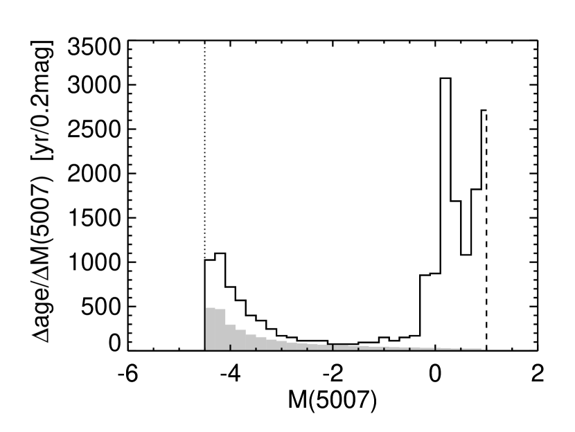
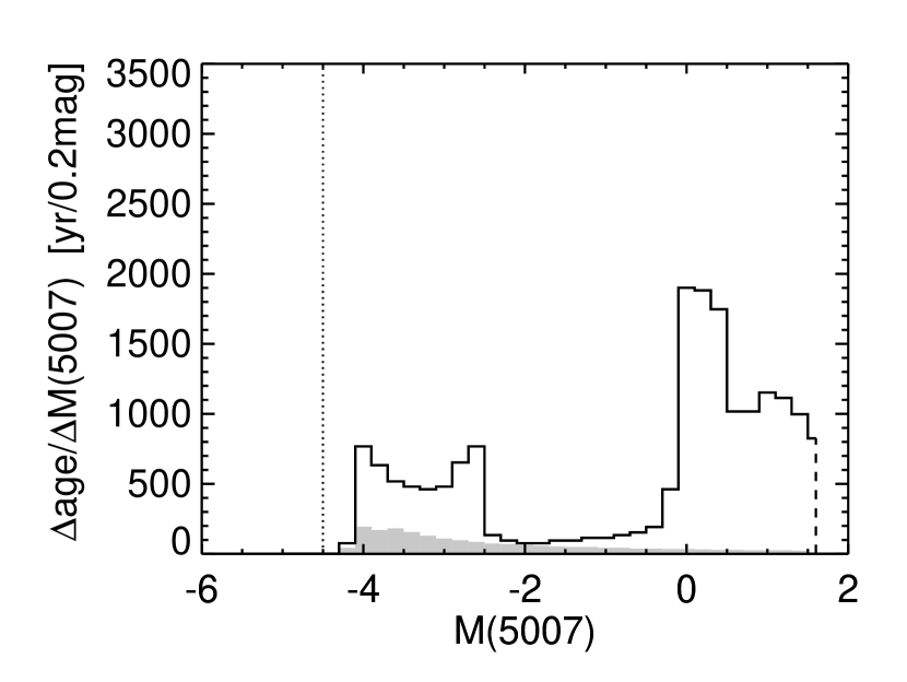
Figure 16: Histograms of two individual [O iii] 5007 Å luminosity function proxies, $\Delta age/\Delta M(5007)$, computed for a central star of 0.605 M_☉ with two different initial circumstellar envelopes as presented by sequences Nos. 4 (top) and 6 (bottom). Plotted are the total times spent per absolute magnitude bin of 0.20 mag. The gray areas reperesent the contributions from increasing brightness. The observed bright $M(5007)$ cut-off is indicated by the vertical dotted line. The vertical dashed lines at the faint end, $M(5007)\geq 0.5$, indicates that there the distributions are affected by the limited simulation times (cf. Fig. 15, bottom panel).

5.1 Individual contributions to the luminosity function

With our very limited number of detailed evolutionary sequences at hand we are not able to construct a theoretical luminosity function useful for interpreting observations. Our computations are, however, very helpful in elucidating how different combinations of central stars and nebular shells will influence the shape of the luminosity function. To this end, we converted the ‘evolutionary’ tracks from Fig. 15 (bottom panel) into histograms giving the expected lifetime of a model per specified magnitude interval – this presentation being a proxy for the (individual) luminosity function of each sequence. In the following figures we preferred a linear ordinate as to facilitate the visualisation of the correspondences with the bottom panel of Fig. 15. The usual logarithmic presentation can be found below.

At first we illustrate in Fig. 16 the influence of two different nebular configurations coupled the the same stellar model of 0.605 M_☉. The different shapes of the luminosity function seen in the figure are then entirely due to the different development of the optical depths, which in turn is the consequence of the different initial configurations with respect of density distribution and total mass (cf. Sect. 2.1).

The optically thick case (top panel) is characterised by an U-shaped curve reflecting the evolution of the whole system: one maximum corresponds to the bright turning point close to $M(5007)\simeq-4.5$ mag, the other at the faint end is due to the strongly reduced evolutionary speed when the central star enters the white-dwarf ‘cooling’ path. In the optically thin case (bottom panel) the luminosity function has a flatter shape at the bright end, combined with a ‘recombination peak’ at $\simeq-2.7$ mag. At the faint end, after recombination, the luminosity evolution is modified by re-ionisation. (cf. Fig. 15, bottom panel). This faint part of the luminosity function, however, is of no observational interest.

In the optically thick case (top panel) the evolution towards maximum [O iii] line emission contributes about 50 % to the total luminosity function except around ${M(5007)\simeq-2}$ mag where this fraction is close to 100 %. In the optically thin case (bottom), the evolution towards maximum line emission contributes much less to the total luminosity function. Both models populate the region of the bright cut-off, $M(5007)=-4.0\ldots-4.5$ mag, but for quite different periods: 2900 yr in the optically thick case (top, No. 4) but only about 800 yr for the sequence No. 6 (bottom) whose models spend, in turn, much more time at medium brightnesses between $M(5007)\simeq-3\dots-4$. The deep depression between $M(5007)\simeq-2.5$ and 0 mag common for both luminosity functions is produced by the rapid luminosity drop of the central star (cf. also Fig. 15).

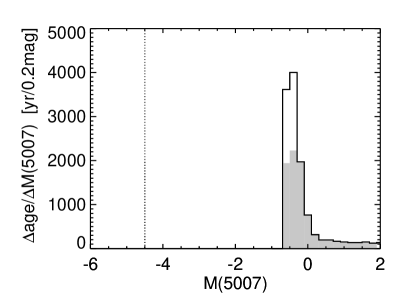
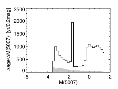
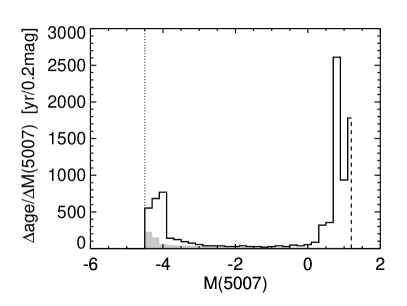
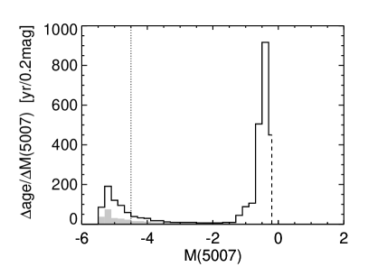
Figure 17: The same as in Fig. 16, but for 0.565 M_☉, (sequence No. 22, top left), 0.595 M_☉, (sequence No. 6a, top right), 0.625 M_☉, (sequence No. 8, bottom left), and 0.696 M_☉, (sequence No. 10, bottom right). Note the different ordinate ranges!

The luminosity functions (resp. their proxies) of the other sequences from Table 2 are shown in Fig. 17. This figure demonstrates how sensitively the bright end of each individual luminosity function depends on the mass of the central star, viz. the speed of its evolution, and the time variation of the optical depth of the nebular shell, determined by gas density and expansion rate. Low-mass objects with, e.g. 0.565 M_☉, and optically very thin nebular envelopes, are contributing only a narrow but rather faint magnitude interval (top left panel). A typical object with a central star close to 0.6 M_☉ becomes much brighter in $M(5007)$, but fails to reach the observed cut-off because the shell becomes optically thin. Recombination peaks are in no case bright enough to contribute to the bright cut-off at $-4.5$ mag. Shells around more massive, i.e. faster evolving central stars, remain mainly optically thick, and their [O iii] emission is able to reach or to pass the observed $M(5007)$ cut-off, even if the envelope becomes somewhat optically thin, as is the case for the 0.625 M_☉ sequence (bottom left and right).

However, the models with more massive central stars stay brighter than $-4.5$ mag in [O iii] for only a brief period, viz. $\approx 500$ yr for 0.7 M_☉. The border-line models with a 0.625 M_☉ central star remain for about 1500 yr close to $M(5007)\simeq-4.5$ mag. Although PNe with such massive central stars do exist (e.g. NGC~7027), their significance for the bright end of the PNLF can only be determined by detailed population syntheses. In any case, our models predict much longer lifetimes at maximum [O iii] emission than the Marigo et al. (2001) models.

Recently Ciardullo et al. (2005) estimated a time span of $\approx\!500$ yr as a typical period to be spent by PN in the top 0.5 mag of the luminosity function. According to our simulations this time should be, on the average, considerably longer, with the consequence of a corresponding reduction of the fraction of stars with appropriate masses that have to evolve off the main sequence and that will eventually evolve into PNe populating the bright end of the luminosity function.

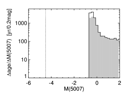
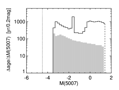
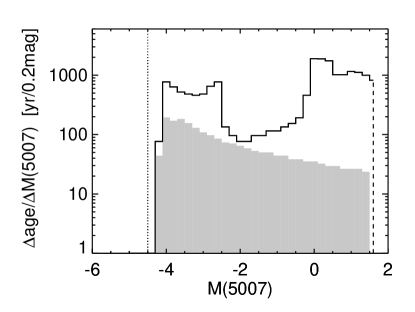
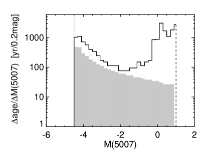
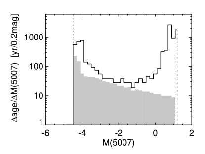
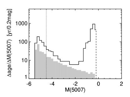
Figure 18: Histograms of the luminosity function proxy, $\Delta age/\Delta M(5007)$, for different simulations with central stars of 0.565 M_☉ (sequence No. 22, top left), 0.595 M_☉ (sequence No. 6a, top right), 0.605 M_☉ (sequence No. 6, middle left), 0.605 M_☉ (sequence No. 4, middle right), 0.625 M_☉ (sequence No. 8, bottom left) and 0.696 M_☉ (sequence No. 10, bottom right). Plotted are the total times spent per absolute magnitude bin of 0.20 mag. The gray histograms illustrate the contributions from increasing line brightness. The dotted vertical line marks the observed bright $M(5007)$ limit. The faint end of the different luminosity functions, indicated by vertical dashed lines, are affected by the limited simulation times (cf. Fig. 15).

In passing we note that our simulations predict also a lower limit of the PNLF at about $M(5007)\simeq 2$ mag. The models at this limit are characterised by white-dwarf central stars with $\simeq$ 200 L_☉ and slowly re-ionising nebulae (Fig. 15, bottom panel).

The observed luminosity functions are usually plotted on a logarithmic scale. We thus present in Fig. 18 our individual luminosity functions from Figs. 16 and 17 in a logarithmic form. Assuming that the mass distribution of central stars is very narrow and peaked at about 0.6 M_☉, our simulations predict a dip in the PNLF around $M(5007)\simeq-2$  mag. This dip is, of course, the signature of the extremely rapid fading of hydrogen-burning central stars once they have passed their maximum effective temperature.

6 The H$\beta$ luminosity functions

For completeness we discuss here the luminosity functions based on the H$\beta$ line. This recombination line has the advantage that it depends only weakly on the electron temperature and is not afflicted by possible abundance variations like the collisionally excited lines of heavy ions, e.g. oxygen. The disadvantage is that H$\beta$ is usually weaker than [O iii] which limits its use in extragalactic research.

Figure 19: Brightness evolution of the H$\beta$ line for the sequences listed in Table 2 vs. central-star effective temperature (top) and post-AGB age (bottom). The circles indicate the moments when the model nebulae become optically thin in the hydrogen Lyman continuum. Note that the sequences Nos. 4 and 10 remain optically thick during their whole computed evolution, while the nebular models of sequence No. 22 turn into the optically thin stage already at a rather low effective temperature.

Figure 19 is the same as Fig. 15, but for H$\beta$. As in the [O iii] case the brightness increase is rapid while the following decrease occurs more gradually. Of course, the peaks due to recombination as seen in Fig. 15 cannot occur for hydrogen.

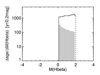
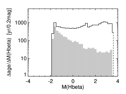
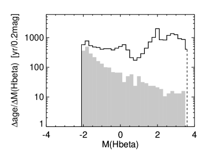
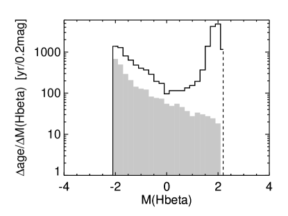
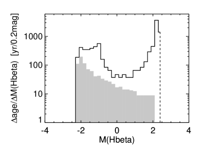
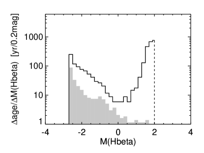
Figure 20: Same as in Fig. 18 but for $M({\rm H}\beta)$.

The brightness evolution of H$\beta$ is converted into the luminosity function proxy, $\Delta age/\Delta M({\rm H}\beta)$, and the results are shown in Fig. 20. By comparison with Fig. 18 we estimate that $M^{\star}(5007)=-4.5$ corresponds to an H$\beta$ cut-off brightness of $-2.2\ldots-2.1$ mag. Although the H$\beta$ luminosity function is fainter by about 2.5 magnitudes, it has also advantages: it does not directly depend on metallicity. The dependence on the electron temperature is weak, thus also the indirect influence of the metallicity is expected to be modest. The dip due to the fast dimming of the central star is expected at about 0.5 mag.

7 Discussion

Summary

With a set of 1D radiation-hydrodynamics simulations aimed at a better understanding of the formation and evolution of planetary nebulae we were able to investigate how the emission of important lines varies during the central-star’s evolution towards a white-dwarf configuration and how they depend on the different combinations of central-star mass and initial envelope structure. Since the most effective conversion of stellar radiation into line emission occurs only for optically thick shells, it is of paramount importance for the interpretation of luminosity functions to know when and at which evolutionary phase PNe become optically thin or whether they will remain always optically thick.

Based on our simulations with hydrogen-burning post-AGB stellar models we found in particular:

• The optical depth in the Lyman continuum depends sensitively on the detailed nebular density structure and, of course, on the expansion speed. The change of the optical depth with time is also controlled by the time evolution of the stellar parameters. Nebulae around central stars with masses $\la 0.6$ M_☉ become optically thin in the Lyman continuum during the early part of the horizontal evolution across the Hertzsprung-Russell diagram ($T_{\mathrm{eff}}<50\,000\leavevmode\nobreak\ {\rm K}$), in good agreement with the observational facts (see Méndez et al. 1992). Central stars slightly more massive, however, evolve fast enough so that there is a large probability that their nebulae remain optically thick, or at least partially thick, during the high-luminosity part of evolution. For masses $\ga\!0.65$ M_☉ the star evolves already so quickly that it is safe to assume that the nebular shell will never become transparent for UV photons, except maybe when the nebular matter becomes very extended and merges with the surrounding interstellar medium. An example is NGC 7027 which is at present optically thick and has probably never been optically thin before (see discussion in Paper III, ).

• With the oxygen abundance typical for galactic disk PNe, the observed [O iii] cut-off luminosity corresponds to a stellar mass of 0.62 M_☉, provided the PN remains optically thick. If the envelope is thin, the stellar luminosities, and hence the masses, must be larger accordingly. While most PNe are certainly optically thin, the ones that populate the bright end of the PNLF are optically thick, at least partially, with central stars slightly more massive than 0.6 M_☉. Support for this interpretation comes from a PNe sample of the Magellanic Clouds for which we demonstrated that the excitations of the brightest objects in H$\beta$ and [O iii] are exactly explained by optically thick (or only marginally thin) nebular shells around central stars with masses slightly in excess of 0.6 M_☉.

The properties of our hydrodynamical models are at variance with those of Marigo et al. (2001, 2004). Their models attain a maximum [O iii] luminosity when they become optically thick during the stellar luminosity decline well beyond effective temperatures of 100 000 K. Since the conversion of UV energy into [O iii] line emission is there less effective, and since also the stars are well beyond their maximum luminosity, Marigo et al. (2004) state that quite large central-star masses, $\approx\!0.70\dots 0.75$ M_☉, are necessary in order to reach the observed cut-off line luminosity.

We demonstrated, however, that our models are superior to the models used by Marigo et al. (2001, 2004) because the latter suffer from shortcomings based on a too a simple physical description. The success of our models is based on the fact that the hydrodynamical simulations take proper care of the interplay between heating and expansion due to photoionisation by the radiation field and compression by wind interaction. The dynamical effect of photoionisation is of paramount importance because it drives a shock wave through the surrounding AGB material, creating thereby a shell with a high-density outer edge which delays the break-through of the H i/ii ionisation front for some time. Only during the further evolution the inner part of the shell is being compressed into the rim due to the increasing pressure exerted by the hot bubble which is shock-heated by the central-star wind. The shell contains most of the nebular mass and determines the size of the PN and its expansion rate. Any attempts to replace the adequate hydrodynamical treatment of these processes by simpler methods must fail.

Helium burning Wolf-Rayet central stars

The present study rests entirely on nebular models around hydrogen-burning post-AGB models. It is expected that any sample of planetary nebulae is contaminated by objects whose central stars are burning helium while they evolve off the AGB, e.g. by objects with (carbon-rich) Wolf-Rayet central stars with strong stellar emission lines and hydrogen-depleted surfaces. Observationally, they may make up for about 25–30 % of the total PNe population. However, Górny et al. (2004) report a smaller fraction of only about 10 %. Because a convincing theory on the formation and evolution of PNe with Wolf-Rayet central stars is still missing, one can only estimate their possible impact on the PNLF.

Assuming that their mass distribution is about the same as that of the hydrogen-rich central stars, we may use the results of Vassiliadis & Wood (1994) for helium-burning central stars to estimate the expected behaviour of the line emission. The evolution of helium-burning models differs twofold from that of the hydrogen-burning models discussed here:

1. They evolve more slowly through the PN domain which will favour optically thin nebulae.

2. They do not cross the HR diagram with a virtually constant luminosity. Instead, their luminosity decreases such that at $T_{\mathrm{eff}}\simeq 100\,000$ K they are less luminous than hydrogen-burning models of the same mass by about a factor of 2 to 3 . Because of the lower stellar luminosity, a PN with a Wolf-Rayet nucleus of about 0.6 M_☉ is not expected to contribute to the [O iii] cut-off luminosity, even if its nebula shell would be optically thick.

There exists the possibility that hydrogen-burning central stars turn into helium-burning ones by a thermal pulse occurring during the transit to the white-dwarf region. Such a pulse forces the star to return briefly back to the vicinity of the AGB. During this transient evolution the stellar surface may become hydrogen-free by mixing and burning. More details about this so-called ‘born-again’ scenario can be found in Herwig (2001). The likelihood of such late thermal pulses is, however, very low and need not be considered here.

We note in passing that the sample of Galactic PNe used in Fig. 13 contains only nuclei with hydrogen-rich surfaces which are believed to burn hydrogen in a shell. In contrast, the fraction of hydrogen-depleted [WC] central stars for the LMC sample presented in Fig. 14 is not known.

The core-mass luminosity relation

We remind the reader that it is the luminosity of a PN nucleus which can only be determined and which is responsible for the PN’s line emission. Reliable masses are only available for a few cases, but in general they are derived by converting luminosity into a (post-AGB) mass using a core-mass luminosity relation based on canonical evolution theory. This relation was originally found by Paczyński (1970), and our post-AGB models provide a relationship very close to that of Paczyński.

The relationship between luminosity and core mass, or virtually total mass for post-AGB objects, depends also somewhat on the metallicity. The only available set of post-AGB models to date computed for different metallicities is that of Vassiliadis & Wood (1994). A comparison with our models shows that the core-mass luminosity relation of their solar-metallicity models agrees reasonably well with ours. The most metal-poor models ($Z=0.001$) are, however, fainter by $\Delta\log L\simeq 0.05$ in the important region between 0.6 and 0.65 M_☉.

Important is that AGB models which include convective overshoot as introduced by Herwig et al. (1997) show a different behaviour between size and mass of the core as compared to standard evolutionary calculations, resulting also in a different relation between core-mass and luminosity. In particular, an unique relation between core mass and luminosity cannot be derived, and as shown by Herwig et al. (1998), the stellar luminosity may exceed the one predicted by the canonical evolutionary theory in which convective overshoot is ignored. As a consequence, the luminosity of a post-AGB star of given mass may be larger than predicted by Paczyński’s law, but by how much depends in a complicated manner on the dredge-up and mass-loss history on the AGB and cannot presently be answered because of our rather limited understanding of stellar convection. Judging from Herwig et al. (1998) it appears plausible that the masses used in our model simulations could be too large by a few 0.01 M_☉ at most.

The universal [O iii] cut-off luminosity

It is still an enigma why the bright cut-off magnitude of the PNLF is virtually independent of the properties of the parent stellar population like, e.g., metallicity or turn-off mass. With our limited set of model simulations we are certainly not in a position to solve this problem. A detailed knowledge of mass loss and dredge-up along the AGB, as a function of the stellar parameter and the metallicity, is needed for any progress.

One should also consider that the maximum of the conversion efficiency of the [O iii] 5007 Å line decreases with metallicity and shifts also to lower effective temperatures (cf. Fig. 2 in Dopita et al. 1992). For instance, at one tenth of the solar metallicity, the maximum 5007 Å emission occurs at $T_{\mathrm{eff}}\simeq 80\,000$ K, with a conversion efficiency reduced by a factor of about two. The reason is simple: at a lower oxygen abundance, O⁺² occurs as the main ionisation stage already at smaller photon fluxes, i.e. at lower stellar temperatures. The reduction of the oxygen abundance is partly compensated for by a larger electron temperature.

It might well be that the combined influence of all the factors discussed here leads to a universal [O iii] cut-off line luminosity. A satisfying answer, however, is only possible with many more simulations of the kind presented here, with all the discussed issues considered, and is far beyond the present work.