Asymptotic Error Rates in Quantum Hypothesis Testing

Abstract

We consider the problem of discriminating between two different states of a finite quantum system in the setting of large numbers of copies, and find a closed form expression for the asymptotic exponential rate at which the specified error probability tends to zero. This leads to the identification of the quantum generalisation of the classical Chernoff distance, which is the corresponding quantity in classical symmetric hypothesis testing, thereby solving a long standing open problem.

The proof relies on a new trace inequality for pairs of positive operators as well as on a special mapping from pairs of density operators to pairs of probability distributions. These two new techniques have been introduced in [quant-ph/0610027] and [quant-ph/0607216], respectively. They are also well suited to prove the quantum generalisation of the Hoeffding bound, which is a modification of the Chernoff distance and specifies the optimal achievable asymptotic error rate in the context of asymmetric hypothesis testing. This has been done subsequently by Hayashi [quant-ph/0611013] and Nagaoka [quant-ph/0611289] for the special case where both hypotheses have full support.

Moreover, quantum Stein’s Lemma and quantum Sanov’s theorem may be derived directly from quantum Hoeffding bound combining it with a result obtained recently in [math/0703772].

The goal of this paper is to present the proofs of the above mentioned results in a unified way and in full generality (allowing hypothetic states with different supports) using mainly the techniques from [quant-ph/0607216] and [quant-ph/0610027].

Additionally, we give an in-depth treatment of the properties of the quantum Chernoff distance. We argue that, although it is not a metric, it is a natural distance measure on the set of density operators, due to its clear operational meaning.

1 Introduction

One of the basic tasks in information theory is discriminating between two different information sources, modelled by (time-discrete) stochastic processes. Given a source that generates independent, identically distributed (i.i.d.) random variables, according to one out of two possible probability distributions, the task is to determine which distribution is the true one, and to do so with minimal error, whatever error criterion one chooses.

This basic decision problem has an equally basic quantum-informational incarnation. Given an information source that emits quantum systems (particles) independently and identically prepared in one out of two possible quantum states, figure out which state is the true one, with minimal error probability.

In both settings, we’re dealing with two hypotheses, each one pertaining to one law represented by a probability distribution or a quantum state, respectively, and the discrimination problem is thus a particular instance of a hypothesis testing problem.

In hypothesis testing, one considers a null hypothesis and an alternative hypothesis. The alternative hypothesis is the one of interest and states that “something significant is happening”, for example, a cell culture under investigation is coming from a malignant tumor, or some case of flu is the avian one, or an e-mail attachment is a computer virus. In contrast, the null hypothesis corresponds to this not being the case; the cells are normal ones, the flu can be treated with an aspirin, and the attachment is just a nice picture. This is inherently an asymmetric situation, and Neyman and Pearson introduced the idea of similarly making a distinction between type I and type II errors.

• The type I error or “false positive”, denoted by $\alpha$, is the error of accepting the alternative hypothesis when in reality the null hypothesis holds and the results can be attributed merely to chance.

• The type II error or “false negative”, denoted by $\beta$, is the error of accepting the null hypothesis when the alternative hypothesis is the true state of nature.

The costs associated to the two types of error can be widely different, or even incommensurate. For example, in medical diagnosis, the type I error corresponds to diagnosing a healthy patient with a certain affliction, which can be an expensive mistake, causing a lot of grievance. On the other hand, the type II error may correspond to declaring a patient healthy while in reality (s)he has a life-threatening condition, which can be a fatal mistake.

To treat the state discrimination problem as a hypothesis test, we assign the null hypothesis to one of the two states and the alternative hypothesis to the other one. If all we want to know is which one of the two possible states we are observing, the mathematical treatment is completely symmetric under the interchange of these two states. It therefore fits most naturally in the setting of symmetric hypothesis testing, where no essential distinction is made between the two kinds of errors. To wit, in symmetric hypothesis testing, one considers the average, or Bayesian, error probability $P_{e}$, defined as the average of $\alpha$ and $\beta$ weighted by the prior probabilities of the null and the alternative hypothesis, respectively.

This paper will be concerned with symmetric as well as with asymmetric quantum hypothesis testing. Since we have developed the main techniques in the symmetric setting we will start with this case and address the asymmetric setting at the end.

The optimal solution to the symmetric classical hypothesis test is given by the maximum-likelihood (ML) test. Starting from the outcomes of an experiment involving $n$ independent draws from the unknown distribution, one calculates the conditional probabilities (likelihoods) that these outcomes can be obtained when the distribution is the one of the null hypothesis and the one of the alternative hypothesis, respectively. One decides then on the hypothesis for which the conditional probability is the highest. I.e. if the likelihood ratio is higher than 1, the null hypothesis is rejected, otherwise it is accepted.

In the quantum setting, the experiment consists of preparing $n$ independent copies of a quantum system in an unknown state, which is either $\rho$ or $\sigma$, and performing an optimal measurement on them. We assume that the quantum systems are finite, implying that the states are associated to density operators on a finite-dimensional complex Hilbert space. Under the null hypothesis, the combined $n$ copies correspond to an $n$-fold tensor product density operator $\rho^{\otimes n}$, while under the alternative hypothesis, the associated density operator is $\sigma^{\otimes n}$. The null hypothesis is then accepted or rejected according to the outcome of the measurement and the specified decision rule. The task of finding this optimal measurement is so fundamental that it was one of the first problems considered in the field of quantum information theory; it was solved in the one-copy case more than 30 years ago by Helstrom and Holevo helstrom ; holevo . We refer to the generalised ML-tests as Holevo-Helstrom tests. In the special case of equal priors, the associated minimal probability of error achieved by the optimal measurement can be calculated from the trace norm distance between the two states:

$$P_{e,n}^{*}(\rho,\sigma)=\frac{1}{2}(1-\|\rho^{\otimes n}-\sigma^{\otimes n}\|_{1}/2),$$ (1)

where $\|A\|_{1}:=\mathop{\rm Tr}\nolimits|A|$ denotes the trace norm.

Going back to the classical case again, in a seminal paper, H. Chernoff chernoff investigated the so-called asymptotical efficiency of a class of statistical tests, which includes the likelihood ratio test mentioned before. The probability of error $P_{e,n}$ in discriminating two probability distributions decreases exponentially in $n$, the number of draws from the distribution: $P_{e,n}\sim\exp(-\xi n)$. For finite $n$ this is a rather crude approximation. However, as $n$ grows larger one finds better and better agreement, and the exponent $\xi$ becomes meaningful in the asymptotic limit. The asymptotical efficiency is exactly the asymptotic limit of this exponent.

Chernoff was able to derive an (almost) closed expression for this asymptotic efficiency, which was later named eponymously in his honour. For two discrete probability distributions $p$ and $q$, this expression is given by

$$\xi_{CB}(p,q):=-\log\left(\inf_{0\leq s\leq 1}\sum_{i}p(i)^{1-s}q(i)^{s}\right),$$ (2)

which is of closed form but for a single variable minimisation. This quantity goes under the alternative names of Chernoff distance, Chernoff divergence and Chernoff information.

While Chernoff’s main purpose was to use this asymptotic efficiency measure to compare the power of different tests – the mathematically optimal test need not always be the most practical one – it can also be used as a distinguishability measure between the distributions (states) of the two hypotheses. Indeed, fixing the test, its efficiency for a particular pair of distributions gives a meaningful indication of how well these two distributions can be distinguished by that test. This is especially meaningful if the applied test is the optimal one.

A quantum generalisation of Chernoff’s result is highly desirable. Given the large amount of experimental effort in the context of quantum information processing to prepare and measure quantum states, it is of fundamental importance to have a theory that allows to discriminate different quantum states in a meaningful way. Despite considerable effort, however, the quantum generalisation of the Chernoff distance has until recently remained unsolved.

In the previous papers, szkola and spain , this issue was finaly settled and the asymptotic error exponent was identified, when the optimal Holevo-Helstrom strategy for discriminating between the two states is used, by proving that the following version of the Chernoff distance

$$\xi_{QCB}(\rho,\sigma):=-\log\left(\inf_{0\leq s\leq 1}\mathop{\rm Tr}\nolimits[\rho^{1-s}\sigma^{s}]\right),$$ (3)

has the same operational meaning as its classical counterpart: It specifies the asymptotic rate exponent of the minimal error probability $P_{e,n}^{*}$ (recall definition (1)). Remarkably, it looks like an almost naïve generalisation of the classical expression (2).

We remark that in the literature different extensions of the classical expression have been considered. Indeed, when insisting only on the compatibility with the classical Chernoff distance, there is in principle an infinitude of possiblities. Among those, three especially promising candidate expressions had been put forward by Ogawa and Hayashi hayashi , who studied their relations and found that there exists an increasing ordering between them. Incidentally, the second candidate coincides with (3) and thus turns out to be the correct one.

Kargin kargin gave lower and upper bounds on the optimal error exponent $\xi$ in terms of the fidelity between the two density operators and found that Ogawa and Hayashi’s third candidate (in their increasing arrangement) is a lower bound on the optimal error exponent for faithful states, i.e. it is an achievable rate. Hayashi hayashibook made progress regarding (3), by showing that for $s=1/2$, $-\log\mathop{\rm Tr}\nolimits[\rho^{1-s}\sigma^{s}]$ is also an achievable error exponent.

The proof of our main result consists of two parts. In the optimality part, which was first presented in szkola , we show that for any test the (Bayesian) error rate $-\frac{1}{n}\log P_{e,n}$ cannot be made arbitrary large but is asymptotically bounded above by $\xi_{QCB}$. In the achievability part, first put forward in spain , we prove that under the Holevo-Helstrom strategy the bound is actually attained in the asymptotic limit, i.e.

$$\limsup_{n\to\infty}\left(-\frac{1}{n}\log P^{\ast}_{e,n}\right)\geq\xi_{QCB}.$$

It is the purpose of this paper to give a complete, detailed, and unified account of these results. We will present the complete proof in Section 3. Moreover, we give an in-depth treatment of the properties of the quantum Chernoff distance in Section 4. More precisely, we show that it defines a distance measure between quantum states.

Distinguishability measures between quantum states have been used in a wide variety of applications in quantum information theory. The most popular of such measures seems to be Uhlmann’s fidelity Uhlman , which happens to coincide with the quantum Chernoff distance when one of the states is pure. The trace norm distance $\|\rho-\sigma\|_{1}=\mathop{\rm Tr}\nolimits|\rho-\sigma|$ has a more natural operational meaning than the fidelity, but lacks monotonicity under taking tensor powers of its arguments. The problem is that one can easily find states $\rho,\sigma,\rho^{\prime},\sigma^{\prime}$ such that $\|\rho-\sigma\|_{1}<\|\rho^{\prime}-\sigma^{\prime}\|_{1}$ but $\|\rho^{\otimes 2}-\sigma^{\otimes 2}\|_{1}>\|\rho^{\prime\otimes 2}-\sigma^{\prime\otimes 2}\|_{1}$. This already happens in the classical setting: take the following 2-dimensional diagonal states

$$\rho={\left(\begin{array}[]{cc}1/4&0\\ 0&3/4\end{array}\right)},\sigma={\left(\begin{array}[]{cc}3/4&0\\ 0&1/4\end{array}\right)},\rho^{\prime}={\left(\begin{array}[]{cc}0&0\\ 0&1\end{array}\right)},\sigma^{\prime}={\left(\begin{array}[]{cc}b&0\\ 0&1-b\end{array}\right)},$$

where $1-1/\sqrt{2}<b<1/2$. Then $\|\rho-\sigma\|_{1}=1>2b=\|\rho^{\prime}-\sigma^{\prime}\|_{1}$, while $\|\rho^{\otimes 2}-\sigma^{\otimes 2}\|_{1}=1<2b(2-b)=\|\rho^{\prime\otimes 2}-\sigma^{\prime\otimes 2}\|_{1}$. The quantum Chernoff distance characterises the exponent arising in the asymptotic behaviour of the trace norm distance, in the case of many identical copies, and therefore by construction does not suffer from this problem. As such, the quantum Chernoff distance can be considered as a kind of regularisation of the trace norm distance. For the above-mentioned states, $\xi_{QCB}(\rho,\sigma)=-\log(\sqrt{3}/2)$ (optimal $s=1/2$) and $\xi_{QCB}(\rho^{\prime},\sigma^{\prime})=-\log(1-b)$ (optimal $s=1$).

A related problem that attracted a lot of attention in the field of quantum information theory was to identify the relative entropy between two quantum states. An information-theoretical way of looking at the classical relative entropy between two probability distributions, or Kullback-Leibler distance, is that it characterises the inefficiency of compressing messages from a source $p$ using an algorithm that is optimal for a source $p^{\prime}$ (i.e. yields the Shannon information bound for that source). Phrased differently, it quantifies the way one could cheat by telling that the given probability distribution is $p$ while the real one is $p^{\prime}$. By proving a quantum version of Stein’s lemma hiaipetz ; ogawa , it has been shown that the quantum relative entropy, as introduced by Umegaki, has exactly the same operational meaning.

When using the relative entropy to distinguish between states, one faces the problem that it is not continuous and is asymmetric under exchange of its arguments, and therefore it does not represent a distance measure in mathematically strict manner. Furthermore, for pure states, the quantum relative entropy is not very useful, since it is either 0 (when the two states are identical) or infinite (when they are not). In contrast, the quantum Chernoff distance seems to be much more natural in many situations.

On the other hand, (quantum) relative entropy is a crucial notion in asymmetric hypothesis testing. There it obtains an operational meaning as the best achievable asymptotic rate of type II errors. Its properties, which are problematic for a candidate for a distance measure, reflect the asymmetry between the null and alternative hypothesis arising from treating the type-I and type-II errors in a different way. As exemplified by the medical diagnosis case mentioned above, the type II error is the one that should be avoided at all costs. Hence, one puts a constraint $\alpha<\epsilon$ on the type I error, and minimises the $\beta$-rate. One obtains that the optimal $\beta$-rate is the relative entropy of the null hypothesis w.r.t. the alternative, independent of the constrained $\epsilon$. The mathematical derivation of this statement goes under the name of Stein’s Lemma. When the constraint consists of a lower bound on the asymptotic exponential rate of the type II error, one obtains what is called the Hoeffding bound.

Asymmetric hypothesis testing has been subject to a quantum theoretical treatment much earlier, although it is a much less natural setting for the basic state discrimination problem. The quantum generalisation of Stein’s Lemma was first obtained by Hiai and Petz hiaipetz . Its optimality part was then strengthened by Ogawa and Nagaoka in ogawa . In the last few years there has been a lot of progress extending the statement of the lemma in different directions. In qSanov the minimal relative entropy distance from a set of quantum states, the null hypothesis, w.r.t. a reference quantum state, the alternative, has been fixed as the best achievable asymptotic rate of the type II errors, see also hayashi:universal_stein . This may be seen as a quantum generalisation of Sanov’s theorem. In a recent paper qSanov2 an extension of this result to the case where the hypotheses correspond to sources emitting correlated (not necessarily i.i.d.) classical or quantum data has been given. Additionally, an equivalence relation between the achievability part in (quantum) Stein’s Lemma and (quantum) Sanov’s Theorem has been derived.

Just a few months after the appearance of szkola ; spain , the techniques pioneered in those two papers were used to find a quantum generalisation of the Hoeffding bound under the implicit assumption of equivalent hypotheses, i.e. for states with coinciding supports, thereby (partially) solving another long-standing open problem in quantum hypothesis testing. Just as in the case of the Chernoff distance, the Hoeffding bound contains $\sum_{i}p(i)^{1-s}q(i)^{s}$ as a sub-expression, and the quantum generalisation of the Hoeffding bound is obtained by replacing this sub-expression by $\mathop{\rm Tr}\nolimits[\rho^{1-s}\sigma^{s}]$. The optimality of the bound (also called the “converse part”) was proven by Nagaoka nagaoka06 , while its achievability (the “direct part”) was found by Hayashi hayashi06 . Using the same techniques, Hayashi also gave a simple proof of the achievability part of the quantum Stein’s Lemma, in that same paper. In Section 5 we first formulate and prove an extended version of the classical Hoeffding bound, which allows nonequivalent hypotheses. Secondly, we present a complete proof of the quantum Hoeffding bound in a unified way. Moreover, we derive quantum Stein’s Lemma as well as quantum Sanov’s Theorem from the quantum Hoeffding bound combined with the mentioned equivalence relation proved in qSanov2 .

2 Mathematical Setting and Problem Formulation

We consider the two hypotheses $H_{0}$ (null) and $H_{1}$ (alternative) that a device prepares finite quantum systems either in the state $\rho$ or in the state $\sigma$, respectively. Everywhere in this paper, we identify a state with a density operator, i.e. a positive trace $1$ linear operator on a finite-dimensional Hilbert space $\mathcal{H}$ associated to the type of the finite quantum system in question. Since the (quantum) Chernoff distance arises naturally in a Bayesian setting, we supply the prior probabilities $\pi_{0}$ and $\pi_{1}$, which are positive quantities summing up to 1; we exclude the degenerate cases $\pi_{0}=0$ and $\pi_{1}=0$ because these are trivial.

Physically discriminating between the two hypotheses corresponds to performing a generalised (POVM) measurement on the quantum system. In analogy to the classical proceeding one accepts $H_{0}$ or $H_{1}$ according to a decision rule based on the outcome of the measurement. There is no loss of generality assuming that the POVM consists of only two elements, which we denote by $\{\mathrm{\leavevmode\hbox{\small 1\normalsize\kern-3.30002pt1}}-\Pi,\Pi\}$, where $\Pi$ may be any linear operator on $\mathcal{H}$ with $0\leq\Pi\leq\mathrm{\leavevmode\hbox{\small 1\normalsize\kern-3.30002pt1}}$. We will mostly make reference to this POVM by its $\Pi$ element, the one corresponding to the alternative hypothesis. The type-I and type-II error probabilities $\alpha$ and $\beta$ are the probabilities of mistaking $\sigma$ for $\rho$, and vice-versa, and are given by

$$\alpha := \mathop{\rm Tr}\nolimits[\Pi\rho]$$

$$\beta := \mathop{\rm Tr}\nolimits[(\mathrm{\leavevmode\hbox{\small 1\normalsize\kern-3.30002pt1}}-\Pi)\sigma].$$

The average error probability $P_{e}$ is given by

$$P_{e}=\pi_{0}\alpha+\pi_{1}\beta=\pi_{0}\mathop{\rm Tr}\nolimits[\Pi\rho]+\pi_{1}\mathop{\rm Tr}\nolimits[(\mathrm{\leavevmode\hbox{\small 1\normalsize\kern-3.30002pt1}}-\Pi)\sigma].$$ (4)

The Bayesian distinguishability problem consists in finding the $\Pi$ that minimises $P_{e}$. A special case is the symmetric one where the prior probabilities $\pi_{0},\pi_{1}$ are equal.

Before we proceed, let us first introduce some basic notations. Abusing terminology, we will use the term ‘positive’ for ‘positive semi-definite’ (denoted $A\geq 0$). We employ the positive semi-definite ordering on the linear operators on $\mathcal{H}$ throughout, i.e. $A\geq B$ iff $A-B\geq 0$. For each linear operator $A\in\mathcal{B}(\mathcal{H})$ the absolute value $|A|$ is defined as $|A|:=(A^{*}A)^{1/2}$. The Jordan decomposition of a self-adjoint operator $A$ is given by $A=A_{+}-A_{-}$, where

$$A_{+}:=(|A|+A)/2,\qquad A_{-}:=(|A|-A)/2$$ (5)

are the positive part and negative part of $A$, respectively. Both parts are positive by definition, and $A_{+}A_{-}=0$.

There is a very useful variational characterisation of the trace of the positive part of a self-adjoint operator $A$:

$$\mathop{\rm Tr}\nolimits[A_{+}]=\max_{X}\{\mathop{\rm Tr}\nolimits[AX]:0\leq X\leq\mathrm{\leavevmode\hbox{\small 1\normalsize\kern-3.30002pt1}}\}.$$ (6)

In other words, the maximum is taken over all positive contractive operators. Since the extremal points of the set of positive contractive operators are exactly the orthogonal projectors, we also have

$$\mathop{\rm Tr}\nolimits[A_{+}]=\max_{P}\{\mathop{\rm Tr}\nolimits[AP]:P\geq 0,P=P^{2}\}.$$ (7)

The maximiser on the right-hand side is the orthogonal projector onto the range of $A_{+}$.

We can now easily prove the quantum version of the Neyman-Pearson Lemma.

Lemma 1 (Quantum Neyman-Pearson)

Let $\rho$ and $\sigma$ be density operators associated to hypotheses $H_{0}$ and $H_{1}$, respectively. Let $T$ be a fixed positive number. Consider the POVM with elements $\{\mathrm{\leavevmode\hbox{\small 1\normalsize\kern-3.30002pt1}}-\Pi^{*},\Pi^{*}\}$ where $\Pi^{*}$ is the projector onto the range of $(T\sigma-\rho)_{+}$, and let $\alpha^{*}=\mathop{\rm Tr}\nolimits[\Pi^{*}\rho]$ and $\beta^{*}=\mathop{\rm Tr}\nolimits[(\mathrm{\leavevmode\hbox{\small 1\normalsize\kern-3.30002pt1}}-\Pi^{*})\sigma]$ be the associated errors. For any other POVM $\{\mathrm{\leavevmode\hbox{\small 1\normalsize\kern-3.30002pt1}}-\Pi,\Pi\}$, with associated errors $\alpha=\mathop{\rm Tr}\nolimits[\Pi\rho]$ and $\beta=\mathop{\rm Tr}\nolimits[(\mathrm{\leavevmode\hbox{\small 1\normalsize\kern-3.30002pt1}}-\Pi)\sigma]$, we have

$$\alpha+T\beta\geq\alpha^{*}+T\beta^{*}=T-\mathop{\rm Tr}\nolimits[(T\sigma-\rho)_{+}].$$

Thus if $\alpha\leq\alpha^{*}$, then $\beta\geq\beta^{*}$.

Proof. By formulae (6) and (7), for all $0\leq\Pi\leq\mathrm{\leavevmode\hbox{\small 1\normalsize\kern-3.30002pt1}}$ we have $\mathop{\rm Tr}\nolimits[\Pi(T\sigma-\rho)]\leq\mathop{\rm Tr}\nolimits(T\sigma-\rho)_{+}=\mathop{\rm Tr}\nolimits[\Pi^{*}(T\sigma-\rho)]$. In terms of $\alpha,\beta,\alpha^{*},\beta^{*}$, this reads $T(1-\beta)-\alpha\leq T(1-\beta^{*})-\alpha^{*}$, which is equivalent to the statement of the Lemma. ∎

The upshot of this Lemma is that the POVM $\{\mathrm{\leavevmode\hbox{\small 1\normalsize\kern-3.30002pt1}}-\Pi^{*},\Pi^{*}\}$, where $\Pi^{*}$ is the projector on the range of $(T\sigma-\rho)_{+}$, is the optimal one when the goal is to minimise the quantity $\alpha+T\beta$. In symmetric hypothesis testing the positive number $T$ is taken to be the ratio $\pi_{1}/\pi_{0}$ of the prior probabilities.

We emphasize that we have started with the assumption that the physical systems in question are finite systems with an algebra of observables $\mathcal{B}(\mathcal{H})$, i.e. the algebra of linear operators on a finite-dimensional Hilbert space $\mathcal{H}$. This is a purely quantum situation. In the general setting (of statistical mechanics) one associates to a finite physical system, classical or quantum, a finite-dimensional $\ast$-algebra $\mathcal{A}$. Such an algebra has a block representation $\bigoplus_{i=1}^{k}\mathcal{B}(\mathcal{H}_{i})$, i.e. it is a subalgebra of $\mathcal{B}(\mathcal{H})$, where $\mathcal{H}:=\bigoplus_{i=1}^{k}\mathcal{H}_{i}$. If the Hilbert spaces $\mathcal{H}_{i}$ are one-dimensional for all $i=1,\ldots,k$, then $\mathcal{A}$ is ^∗-isomorphic to the commutative algebra of diagonal $(k\times k)$-matrices. This covers the classical case. Now, in view of Lemma 1 it becomes clear that in the context of hypothesis testing there is no restriction assuming that the algebra of observables of the systems in question is $\mathcal{B}(\mathcal{H})$; indeed, the optimally discriminating projectors $\Pi^{*}$ are always in the $\ast$-subalgebra generated by the two involved density operators $\rho$ and $\sigma$. This implies that they are automatically elements of the algebra $\mathcal{A}$ characterising the physical systems. In particular, if the hypotheses correspond to mutually commuting density operators then the problem reduces to a classical one in the sense that the best test $\Pi^{*}$ commutes with the density operators as well. Hence it coincides with the classical ML-test, although there are many more possible tests in $\mathcal{B}(\mathcal{H})$ than in the commutative subalgebra of observables of the classical subsystem.

The basic problem we focus on in this paper is to identify how the error probability $P_{e}$ behaves in the asymptotic limit, i.e. when one has to discriminate between the hypotheses $H_{0}$ and $H_{1}$ on the basis of a large number $n$ of copies of the quantum systems. This means that we have to distinguish between the $n$-fold tensor product density operators $\rho^{\otimes n}$ and $\sigma^{\otimes n}$ by means of POVMs $\{\mathrm{\leavevmode\hbox{\small 1\normalsize\kern-3.30002pt1}}-\Pi_{n},\Pi_{n}\}$ on $\mathcal{H}^{\otimes n}$.

We define the rate limit $s_{R}$ for any positive sequence $(s_{n})$ as

$$s_{R}:=\lim_{n\to\infty}\left(-\frac{1}{n}\log s_{n}\right),$$

if the limit exists. Otherwise we have to deal with the lower and upper rate limits $\underline{s}_{R}$ and $\overline{s}_{R}$, which are the limit inferior and the limit superior of the sequence $(-\frac{1}{n}\log s_{n})$, respectively. In particular, we define the type-I error rate limit and the type-II error rate limit for a sequence $\Pi:=(\Pi_{n})$ of quantum measurements (where, as mentioned, each orthogonal projection $\Pi_{n}$ corresponds to the alternative hypothesis) as

$$\alpha_{R}(\Pi) := \lim_{n\to\infty}\left(-\frac{1}{n}\log\alpha_{n}\right)=\lim_{n\to\infty}\left(-\frac{1}{n}\log\mathop{\rm Tr}\nolimits[\rho^{\otimes n}\Pi_{n}]\right)$$ (8)

$$\beta_{R}(\Pi) := \lim_{n\to\infty}\left(-\frac{1}{n}\log\beta_{n}\right)=\lim_{n\to\infty}\left(-\frac{1}{n}\log\mathop{\rm Tr}\nolimits[\sigma^{\otimes n}(\mathrm{\leavevmode\hbox{\small 1\normalsize\kern-3.30002pt1}}-\Pi_{n})]\right),$$ (9)

if the limits exist. Otherwise we consider the limit inferior and the limit superior $\underline{\alpha}_{R}(\Pi)$ and $\overline{\alpha}_{R}(\Pi)$, respectively. Similar definitions hold in the classical case.

3 Bayesian Quantum Hypothesis Testing: Quantum Chernoff Bound

In this section we consider the Bayesian distinguishability problem. This means the goal is to minimise the average error probability $P_{e}$, which is defined in (4) and can be rewritten as $P_{e}=\pi_{1}-\mathop{\rm Tr}\nolimits[\Pi(\pi_{1}\sigma-\pi_{0}\rho)]$. By the Neyman-Pearson Lemma, the optimal test is given by the projector $\Pi^{*}$ onto the range of $(\pi_{1}\sigma-\pi_{0}\rho)_{+}$, and the obtained minimal error probability is given by

$$P_{e}^{*} = \pi_{1}-\mathop{\rm Tr}\nolimits[(\pi_{1}\sigma-\pi_{0}\rho)_{+}]$$

$$= \pi_{1}-(\pi_{1}-\pi_{0})/2-\mathop{\rm Tr}\nolimits[|\pi_{1}\sigma-\pi_{0}\rho|/2]$$

$$= \frac{1}{2}\left(1-\|\pi_{1}\sigma-\pi_{0}\rho\|_{1}\right),$$

where $\|A\|_{1}=\mathop{\rm Tr}\nolimits|A|$ is the trace norm. We will call $\Pi^{*}$ the Holevo-Helstrom projector.

Next, note that the optimal test to discriminate $\rho$ and $\sigma$ in the case of $n$ copies enforces the use of joint measurements. However, the particular permutational symmetry of $n$-copy states guarantees that the optimal collective measurement can be implemented efficiently (with a polynomial-size circuit) bacon04 , and hence that the minimum probability of error is achievable with a reasonable amount of resources.

We need to consider the quantity

$$P_{e,n}^{*}:=(1-\|\pi_{1}\sigma^{\otimes n}-\pi_{0}\rho^{\otimes n}\|_{1})/2.$$ (10)

It turns out that $P_{e,n}^{*}$ vanishes exponentially fast as $n$ tends to infinity. The theorem below provides the asymptotic value of the exponent $-\frac{1}{n}\log P^{*}_{e,n}$, i.e. the rate limit of $P_{e,n}^{*}$, which turns out to be given by the quantum Chernoff distance. This is our main result.

Theorem 3.1

For any two states $\rho$ and $\sigma$ on a finite-dimensional Hilbert space, occurring with prior probabilities $\pi_{0}$ and $\pi_{1}$, respectively, the rate limit of $P_{e,n}^{*}$, as defined by (10), exists and is equal to the quantum Chernoff distance $\xi_{QCB}$

$$\lim_{n\rightarrow\infty}\left(-\frac{1}{n}\log P_{e,n}^{*}\right)=\xi_{QCB}:=-\log\left(\inf_{0\leq s\leq 1}\mathop{\rm Tr}\nolimits\left(\rho^{1-s}\sigma^{s}\right)\right).$$ (11)

Because the product of two positive operators always has positive spectrum, the quantity $\mathop{\rm Tr}\nolimits[\rho^{1-s}\sigma^{s}]$ is well defined (in the mathematical sense) and guaranteed to be real and non-negative for every $0\leq s\leq 1$. As should be, the expression for $\xi_{QCB}$ reduces to the classical Chernoff distance $\xi_{CB}$ defined by (2) when $\rho$ and $\sigma$ commute.

3.1 Proof of Theorem 3.1: Optimality Part

In this Section, we will show that the best discrimination is specified by the quantum Chernoff distance; that is, $\xi_{QCB}$ is an upper bound on

$$\limsup_{n\rightarrow\infty}\left(-\frac{1}{n}\log P_{e,n}\right)$$

for any sequence of tests $(\Pi_{n})$ and $P_{e,n}:=\pi_{1}-\textrm{Tr }[\pi_{1}\sigma^{\otimes n}-\pi_{0}\rho^{\otimes n}]$.

The proof, which first appeared in szkola , is essentially based on relating the quantum to the classical case by using a special mapping from a pair of $d\times d$ density matrices $(\rho,\sigma)$ to a pair of probability distributions $(p,q)$ on a set of cardinality $d^{2}$.

Let the spectral decompositions of $\rho$ and $\sigma$ be given by

$$\rho=\sum_{i=1}^{d}\lambda_{i}|x_{i}\rangle\langle x_{i}|,\quad\sigma=\sum_{j=1}^{d}\mu_{j}|y_{j}\rangle\langle y_{j}|,$$

where $(|x_{i}\rangle)$ and $(|y_{j}\rangle)$ are two orthonormal bases of eigenvectors and $(\lambda_{i})$ and $(\mu_{j})$ are the corresponding sets of eigenvalues of $\rho$ and $\sigma$, respectively. Then we map these density operators to the $d^{2}$-dimensional vectors

$$p_{i,j}=\lambda_{i}|\langle x_{i}|y_{j}\rangle|^{2},\quad q_{i,j}=\mu_{j}|\langle x_{i}|y_{j}\rangle|^{2},$$ (12)

with $1\leq i,j\leq d$. This mapping preserves a number of important properties:

Proposition 1

With $p_{i,j}$ and $q_{i,j}$ as defined in (12), and $s\in{\mathbb{R}}$,

$$\mathop{\rm Tr}\nolimits[\rho^{1-s}\sigma^{s}] = \sum_{i,j}p_{i,j}^{1-s}q_{i,j}^{s}$$ (13)

$$S(\rho\|\sigma) = H(p\|q).$$ (14)

Here, $S(\rho\|\sigma)$ is the quantum relative entropy defined as

$$S(\rho\|\sigma) := \left\{\begin{array}[]{l}\mathop{\rm Tr}\nolimits[\rho(\log\rho-\log\sigma)],\mbox{ if }\mathop{\rm Supp}\nolimits\rho\leq\mathop{\rm Supp}\nolimits\sigma\\[2.84526pt] +\infty,\mbox{ otherwise,}\end{array}\right.$$ (17)

where $\mathop{\rm Supp}\nolimits\rho$ denotes the support projection of an operator $\rho$, and $H(p\|q)$ is the classical relative entropy, or Kullback-Leibler distance,

$$H(p\|q) := \left\{\begin{array}[]{l}\sum_{i,j}p_{i,j}(\log p_{i,j}-\log q_{i,j}),\mbox{ if }p\ll q\\[2.84526pt] +\infty,\mbox{ otherwise.}\end{array}\right.$$ (20)

Proof. The proof proceeds by direct calculation. For example:

$$\mathop{\rm Tr}\nolimits[\rho^{1-s}\sigma^{s}] = \sum_{i,j}\lambda_{i}^{1-s}\mu_{j}^{s}|\langle x_{i}|y_{j}\rangle|^{2}$$

$$= \sum_{i,j}\lambda_{i}^{1-s}\mu_{j}^{s}|\langle x_{i}|y_{j}\rangle|^{2(1-s)}|\langle x_{i}|y_{j}\rangle|^{2s}$$

$$= \sum_{i,j}p_{i,j}^{1-s}q_{i,j}^{s}.$$

∎

A direct consequence of identity (13) is that $p$ and $q$ are normalised if $\rho$ and $\sigma$ are. Furthermore, tensor powers are preserved by the mapping; that is, if $\rho$ and $\sigma$ are mapped to $p$ and $q$, then $\rho^{\otimes n}$ is mapped to $p^{\otimes n}$ and $\sigma^{\otimes n}$ to $q^{\otimes n}$.

Now define the classical and quantum average (Bayesian) error probabilities $P_{e,c}$ and $P_{e,q}$ as

$$P_{e,c}(\phi,p,\pi_{0},q,\pi_{1}) := \sum_{i}[\pi_{0}\phi(i)p_{i}+\pi_{1}(1-\phi(i))q_{i}]$$ (21)

$$P_{e,q}(\Pi,\rho,\pi_{0},\sigma,\pi_{1}) := \mathop{\rm Tr}\nolimits[\pi_{0}\Pi\rho+\pi_{1}(\mathrm{\leavevmode\hbox{\small 1\normalsize\kern-3.30002pt1}}-\Pi)\sigma],$$ (22)

where $p,q$ are probability distributions, $\rho,\sigma$ are density matrices, and $\pi_{0},\pi_{1}$ are the respective prior probabilities of the two hypotheses. Furthermore, $\phi$ is a non-negative test function $0\leq\phi\leq 1$, and $\Pi$ is a positive semi-definite contraction, $0\leq\Pi\leq\mathrm{\leavevmode\hbox{\small 1\normalsize\kern-3.30002pt1}}$, so that $\{\mathrm{\leavevmode\hbox{\small 1\normalsize\kern-3.30002pt1}}-\Pi,\Pi\}$ forms a POVM.

The main property of the mapping that allows to establish optimality of the quantum Chernoff distance is presented in the following Proposition.

Proposition 2

For all orthogonal projectors $\Pi$ and all positive scalars $\eta_{0},\eta_{1}$ (not necessarily adding up to 1), and for $p$ and $q$ associated to $\rho$ and $\sigma$ by the mapping (12),

$$P_{e,q}(\Pi,\rho,\eta_{0},\sigma,\eta_{1})\geq\frac{1}{2}\inf_{\phi}P_{e,c}(\phi,p,\eta_{0},q,\eta_{1}),$$

where the infimum is taken over all test functions $0\leq\phi\leq 1$.

Note that we have replaced the priors by general positive scalars; this will be useful later on, in proving the optimality of the Hoeffding bound.

Proof. Since $\Pi$ is a projector, one has $\Pi=\Pi\Pi=\sum_{j}\Pi|y_{j}\rangle\langle y_{j}|\Pi$, where the second equality is obtained by inserting a resolution of the identity $\mathrm{\leavevmode\hbox{\small 1\normalsize\kern-3.30002pt1}}=\sum_{j}|y_{j}\rangle\langle y_{j}|$. Likewise, $\mathrm{\leavevmode\hbox{\small 1\normalsize\kern-3.30002pt1}}-\Pi$ is also a projector, and using another resolution of the identity, $\mathrm{\leavevmode\hbox{\small 1\normalsize\kern-3.30002pt1}}=\sum_{i}|x_{i}\rangle\langle x_{i}|$, we similarly get $\mathrm{\leavevmode\hbox{\small 1\normalsize\kern-3.30002pt1}}-\Pi=\sum_{i}(\mathrm{\leavevmode\hbox{\small 1\normalsize\kern-3.30002pt1}}-\Pi)|x_{i}\rangle\langle x_{i}|(\mathrm{\leavevmode\hbox{\small 1\normalsize\kern-3.30002pt1}}-\Pi)$. This yields

$$\mathop{\rm Tr}\nolimits[\Pi\rho] = \sum_{i}\lambda_{i}\mathop{\rm Tr}\nolimits[\Pi|x_{i}\rangle\langle x_{i}|]$$

$$= \sum_{i,j}\lambda_{i}\mathop{\rm Tr}\nolimits[\Pi|y_{j}\rangle\langle y_{j}|\Pi|x_{i}\rangle\langle x_{i}|]$$

$$= \sum_{i,j}\lambda_{i}|\langle x_{i}|\Pi|y_{j}\rangle|^{2},$$

and, similarly,

$$\mathop{\rm Tr}\nolimits[(\mathrm{\leavevmode\hbox{\small 1\normalsize\kern-3.30002pt1}}-\Pi)\sigma] = \sum_{i,j}\mu_{j}|\langle x_{i}|\mathrm{\leavevmode\hbox{\small 1\normalsize\kern-3.30002pt1}}-\Pi|y_{j}\rangle|^{2}.$$

Then the quantum error probability is given by

$$P_{e,q} = \eta_{0}\mathop{\rm Tr}\nolimits[\Pi\rho]+\eta_{1}\mathop{\rm Tr}\nolimits[(\mathrm{\leavevmode\hbox{\small 1\normalsize\kern-3.30002pt1}}-\Pi)\sigma]$$

$$= \sum_{i,j}\eta_{0}\lambda_{i}|\langle x_{i}|\Pi|y_{j}\rangle|^{2}+\eta_{1}\mu_{j}|\langle x_{i}|\mathrm{\leavevmode\hbox{\small 1\normalsize\kern-3.30002pt1}}-\Pi|y_{j}\rangle|^{2}.$$

The infimum of the classical error probability $P_{e,c}$ is obtained when the test function $\phi$ equals the indicator function $\phi=\chi_{\{\eta_{1}q>\eta_{0}p\}}$ (corresponding to the maximum likelihood decision rule); hence, the value of this infimum is given by

$$\inf_{\phi}P_{e,c} = \sum_{i,j}\min(\eta_{0}p_{i,j},\eta_{1}q_{i,j})$$

$$= \sum_{i,j}\min(\eta_{0}\lambda_{i},\eta_{1}\mu_{j})|\langle x_{i}|y_{j}\rangle|^{2}.$$

For a fixed choice of $i,j$, let $a$ be the $2\times 2$ non-negative diagonal matrix

$$a:={\left(\begin{array}[]{cc}\eta_{0}\lambda_{i}&0\\ 0&\eta_{1}\mu_{j}\end{array}\right)},$$

and let $b$ be the 2-vector

$$b:=(\langle x_{i}|\Pi|y_{j}\rangle,\langle x_{i}|\mathrm{\leavevmode\hbox{\small 1\normalsize\kern-3.30002pt1}}-\Pi|y_{j}\rangle).$$

The $i,j$-term in the sum for $P_{e,q}$ can then be written as the inner product $\langle b|a|b\rangle$. Similarly, the factor $|\langle x_{i}|y_{j}\rangle|^{2}$ occurring in the $i,j$-term in the sum for $P_{e,c}$ can then be written as $|b_{1}+b_{2}|^{2}$.

Now we note that $\langle b|b\rangle=\|b\|_{2}^{2}$, while $|b_{1}+b_{2}|^{2}\leq\|b\|_{1}^{2}$. For $d$-dimensional vectors, the inequality $\|b\|_{2}\geq\|b\|_{1}/\sqrt{d}$ holds; in our case, $d=2$. Together with the inequality $a\geq\min(\eta_{0}\lambda_{i},\eta_{1}\mu_{j})\mathrm{\leavevmode\hbox{\small 1\normalsize\kern-3.30002pt1}}_{2}$ this yields

$$\langle b|a|b\rangle\geq\min(\eta_{0}\lambda_{i},\eta_{1}\mu_{j})\langle b|b\rangle\geq\min(\eta_{0}\lambda_{i},\eta_{1}\mu_{j})\frac{1}{2}|b_{1}+b_{2}|^{2}.$$ (23)

Therefore, we obtain, for any $i,j$,

$$\eta_{0}\lambda_{i}|\langle x_{i}|\Pi|y_{j}\rangle|^{2}+\eta_{1}\mu_{j}|\langle x_{i}|\mathrm{\leavevmode\hbox{\small 1\normalsize\kern-3.30002pt1}}-\Pi|y_{j}\rangle|^{2}\geq\frac{1}{2}\min(\eta_{0}\lambda_{i},\eta_{1}\mu_{j})|\langle x_{i}|y_{j}\rangle|^{2}.$$

As this holds for any $i,j$, it holds for the sum over $i,j$, so that a lower bound for the quantum error probability is given by

$$P_{e,q}\geq\frac{1}{2}\sum_{i,j}\min(\eta_{0}p_{i,j},\eta_{1}q_{i,j})=\frac{1}{2}\inf_{\phi}P_{e,c},$$

which proves the Proposition. ∎

Using these properties of the mapping, the proof of optimality of the quantum Chernoff bound is easy.

Proof of optimality of the quantum Chernoff bound. Let hypotheses $H_{0}$ and $H_{1}$, with priors $\pi_{0}$ and $\pi_{1}$, correspond to the product states $\rho^{\otimes n}$ and $\sigma^{\otimes n}$. Using the mapping (12), these states are mapped to the probability distributions $p^{\otimes n}$ and $q^{\otimes n}$. By Proposition 2, the quantum error probability is bounded from below as

$$P_{e,q}(\Pi_{n},\rho^{\otimes n},\pi_{0},\sigma^{\otimes n},\pi_{1})\geq\frac{1}{2}\inf_{\phi_{n}}P_{e,c}(\phi_{n},p^{\otimes n},\pi_{0},q^{\otimes n},\pi_{1}).$$ (24)

By the classical Chernoff bound, the rate limit of the right-hand side is given by

$$-\log\inf_{0\leq s\leq 1}\sum_{i,j}p_{i,j}^{1-s}q_{i,j}^{s}$$

(provided the priors $\pi_{0},\pi_{1}$ are non-zero) and this is, therefore, an upper bound on the rate limit of the optimal quantum error probability. By Proposition 1 the latter expression is equal to $-\log\inf_{0\leq s\leq 1}\mathop{\rm Tr}\nolimits[\rho^{1-s}\sigma^{s}]$, which is what we set out to prove. ∎

In a similar way one can prove the converse part of the quantum Hoeffding bound by relating it to the classical problem in the sense of (12), as already noted by Nagaoka in nagaoka06 . This will be discussed in Section 5.4.

3.2 Proof of Theorem 3.1: Achievability Part

In this Section, we prove the achievability of the quantum Chernoff bound, which is the statement that the error rate limit $\lim_{n\rightarrow\infty}\left(-\frac{1}{n}\log P_{e,n}^{*}\right)$ is not only bounded above by, but is actually equal to the quantum Chernoff distance $\xi_{QCB}$. This can directly be inferred from the following matrix inequality, which first made its appearance in spain :

Theorem 3.2

Let $a$ and $b$ be positive semi-definite operators, then for all $0\leq s\leq 1$,

$$\mathop{\rm Tr}\nolimits[a^{s}b^{1-s}]\geq\mathop{\rm Tr}\nolimits[a+b-|a-b|]/2.$$ (25)

Note that inequality (25) is also interesting from a purely matrix analytic point of view, as it relates the trace norm to a multiplicative quantity in a highly nontrivial and very useful way.

If we specialise this Theorem to states, $a=\sigma$ and $b=\rho$, with $\mathop{\rm Tr}\nolimits\rho=\mathop{\rm Tr}\nolimits\sigma=1$, we obtain

$$Q_{s}+T\geq 1,\qquad 0\leq s\leq 1,$$

where $Q_{s}:=Q_{s}(\rho,\sigma):=\mathop{\rm Tr}\nolimits[\rho^{1-s}\sigma^{s}]$ and $T:=T(\rho,\sigma):=\|\rho-\sigma\|_{1}/2$ is the trace norm distance.

As an aside it is interesting to note that the inequality $Q_{s}+T\geq 1$ is strongly sharp, which means that for any allowed value of $T$ one can find $\rho$ and $\sigma$ that achieve equality. Indeed, take the commuting density operators $\rho=|0\rangle\langle 0|$ and $\sigma=(1-T)|0\rangle\langle 0|+T|1\rangle\langle 1|$, then their trace norm distance is $T$, and $Q_{s}=1-T$.

Proof of achievability of the quantum Chernoff bound from Theorem 3.2.

We will prove the inequality

$$\liminf_{n\rightarrow\infty}\left(-\frac{1}{n}\log P_{e,n}^{*}\right)\geq\xi_{QCB}.$$ (26)

Put $a=\pi_{1}\sigma^{\otimes n}$ and $b=\pi_{0}\rho^{\otimes n}$, so that the right-hand side of (25) turns into

$$(1-\|\pi_{1}\sigma^{\otimes n}-\pi_{0}\rho^{\otimes n}\|_{1})/2=P_{e,n}^{*}.$$

The logarithm of the left-hand side of inequality (25) simplifies to

$$\log(\pi_{0}^{1-s}\pi_{1}^{s})+n\log\left(\mathop{\rm Tr}\nolimits[\rho^{1-s}\sigma^{s}]\right).$$

Upon dividing by $n$ and taking the limit $n\to\infty$, we obtain $\log Q_{s}$, independently of the priors $\pi_{0}$, $\pi_{1}$ (as long as the priors are not degenerate, i.e. are different from 0 or 1). Then (26) follows from the fact that the inequality

$$\liminf_{n\rightarrow\infty}\left(-\frac{1}{n}\log P_{e,n}^{*}\right)\geq-\log Q_{s}$$

holds for all $s\in[0,1]$ and we can replace the right-hand side by $\xi_{QCB}$.∎

Proof of Theorem 3.2.

The left-hand and right-hand sides of (25) look very disparate, but they can nevertheless be brought closer together by expressing $a+b-|a-b|$ in terms of the positive part $(a-b)_{+}$. The inequality (25) is indeed equivalent to

$$\mathop{\rm Tr}\nolimits[a-a^{s}b^{1-s}] \leq \mathop{\rm Tr}\nolimits[a-(a+b-|a-b|)/2]$$ (27)

$$= \mathop{\rm Tr}\nolimits[(a-b+|a-b|)/2]$$

$$= \mathop{\rm Tr}\nolimits[(a-b)_{+}].$$

At this point we mention another equivalent formulation of this inequality, which will be used later in the proof of the achievability of the quantum Hoeffding bound. With $\Pi$ the projector on the range of $(a-b)_{+}$, we can write:

$$\mathop{\rm Tr}\nolimits[a^{s}b^{1-s}]\geq\mathop{\rm Tr}\nolimits[\Pi b+(\mathrm{\leavevmode\hbox{\small 1\normalsize\kern-3.30002pt1}}-\Pi)a].$$ (28)

What we do next is strengthening the inequality (27) by replacing its left-hand side by an upper bound, and its right-hand side by a lower bound. Since, for any self-adjoint operator $H$, we have $H\leq H_{+}$, we can write

$$\mathop{\rm Tr}\nolimits[a-a^{s}b^{1-s}]=\mathop{\rm Tr}\nolimits[a^{s}(a^{1-s}-b^{1-s})] \leq \mathop{\rm Tr}\nolimits[a^{s}(a^{1-s}-b^{1-s})_{+}]$$

$$= \mathop{\rm Tr}\nolimits[a^{s}\Pi^{(s)}(a^{1-s}-b^{1-s})]$$

$$= \mathop{\rm Tr}\nolimits[\Pi^{(s)}(a-b^{1-s}a^{s})],$$

where $\Pi^{(s)}$ is the projector on the range of $(a^{1-s}-b^{1-s})_{+}$. Likewise,

$$\mathop{\rm Tr}\nolimits[\Pi^{(s)}(a-b)]\leq\mathop{\rm Tr}\nolimits[(a-b)_{+}],$$

because $\mathop{\rm Tr}\nolimits[(a-b)_{+}]$ is the maximum of $\mathop{\rm Tr}\nolimits[\Pi(a-b)]$ over all orthogonal projections $\Pi$. Inequality (25) would thus follow if, for that particular $\Pi^{(s)}$,

$$\mathop{\rm Tr}\nolimits[\Pi^{(s)}(a-b^{1-s}a^{s})]\leq\mathop{\rm Tr}\nolimits\Pi^{(s)}(a-b).$$

The benefit of this reduction is obvious, as after simplification we get the much nicer statement

$$\mathop{\rm Tr}\nolimits[\Pi^{(s)}b^{1-s}(a^{s}-b^{s})]\geq 0.$$

Equally obvious, though, is the risk of this strengthening; it could very well be a false statement. Nevertheless, we show its correctness below.

It is interesting to note the meaning here of this strengthening in the context of the optimal hypothesis test, i.e. when $a=\sigma^{\otimes n}$ and $b=\rho^{\otimes n}$. While the Holevo-Helstrom projectors $\Pi^{*}_{n}$ are optimal for every finite value of $n$, we can use other projectors that are suboptimal but reach optimality in the asymptotic sense. Here we are indeed using $\Pi^{(s^{*})}$, the projector on the range of $(a^{1-s^{*}}-b^{1-s^{*}})_{+}$, where $s^{*}$ is the minimiser of $\mathop{\rm Tr}\nolimits[\rho^{1-s}\sigma^{s}]$ over $[0,1]$, if it exists. Otherwise we have to use the Holevo-Helstrom projector.

In the next few steps we will further reduce the statement by reformulating the matrix powers in terms of simpler expressions. One can immediately absorb one of them into $a$ and $b$ via appropriate substitutions. As we certainly don’t want a power appearing in the definition of the projector $\Pi^{(s)}$, we are led to apply the substitutions

$$A=a^{1-s},\quad B=b^{1-s},\quad t=s/(1-s).$$

This yields a value of $t$ between 0 and 1 only when $0\leq s\leq 1/2$. However, this is no restriction since the case $1/2\leq s\leq 1$ can be treated in a completely similar way after applying an additional substitution $s\to 1-s$.

Inequality (25) is thus implied by the Lemma below, which ends the proof of Theorem 3.2.∎

Lemma 2

For matrices $A,B\geq 0$, a scalar $0\leq t\leq 1$, and denoting by $P$ the projector on the range of $(A-B)_{+}$, the following inequality holds:

$$\mathop{\rm Tr}\nolimits[PB(A^{t}-B^{t})]\geq 0.$$ (29)

Proof. To deal with the $t$-th matrix power, we use an integral representation (see, for example bhatia (V.56)). For scalars $a\geq 0$ and $0\leq t\leq 1$,

$$a^{t}=\frac{\sin(t\pi)}{\pi}\int_{0}^{+\infty}dx\,\,x^{t-1}\,\,\frac{a}{a+x}.$$

For other values of $t$ this integral does not converge. This integral can be extended to positive operators in the usual way:

$$A^{t}=\frac{\sin(t\pi)}{\pi}\int_{0}^{+\infty}dx\,\,x^{t-1}\,\,A(A+x\mathrm{\leavevmode\hbox{\small 1\normalsize\kern-3.30002pt1}})^{-1}.$$

To deal with non-invertible $A$ (arising when the states $\rho$ and $\sigma$ are not faithful), we define $\lim_{x\to 0}A(A+x\mathrm{\leavevmode\hbox{\small 1\normalsize\kern-3.30002pt1}})^{-1}=\mathrm{\leavevmode\hbox{\small 1\normalsize\kern-3.30002pt1}}$.

The potential benefit of this integral representation is that statements about the integral might follow from statements about the integrand, which is a simpler quantity.

Applying the integral representation to $A^{t}$ and $B^{t}$, we get

$$\mathop{\rm Tr}\nolimits[PB(A^{t}-B^{t})]=\frac{\sin(t\pi)}{\pi}\int_{0}^{+\infty}dx\,\,x^{t-1}\mathop{\rm Tr}\nolimits[PB(A(A+x)^{-1}-B(B+x)^{-1})].$$

If the integrand is positive for all $x>0$ (it is zero for $x=0$), then the whole integral is positive. The Lemma follows if indeed we have

$$\mathop{\rm Tr}\nolimits[PB(A(A+x)^{-1}-B(B+x)^{-1})]\geq 0.$$

As a further reduction, we note that a difference can be expressed as an integral of a derivative:

$$f(a)-f(b)=f(b+(a-b))-f(b)=\int_{0}^{1}dt\,\,\frac{d}{dt}f(b+(a-b)t).$$

Here, we will apply this to the expression $A(A+x)^{-1}-B(B+x)^{-1}$. Let $\Delta=A-B$. Then

$$A(A+x)^{-1}-B(B+x)^{-1} = \int_{0}^{1}dt\,\,\frac{d}{dt}(B+t\Delta)(B+t\Delta+x)^{-1}.$$

The potential benefit is again that the required statement might follow from a statement about the integrand, which is a simpler quantity provided one is able to calculate the derivative explicitly. In this case we are not dealing with a stronger statement, because the statement has to hold for the derivative anyway (when $A$ is close to $B$).

In the present case, we can indeed calculate the derivative:

$$\frac{d}{dt}(B+t\Delta)(B+t\Delta+x)^{-1} = x\,\,(B+t\Delta+x)^{-1}\,\,\Delta\,\,(B+t\Delta+x)^{-1}.$$

Therefore,

$$\mathop{\rm Tr}\nolimits[PB(A(A+x)^{-1}-B(B+x)^{-1})]$$

$$= x\,\int_{0}^{1}dt\,\,\mathop{\rm Tr}\nolimits[PB(B+t\Delta+x)^{-1}\Delta(B+t\Delta+x)^{-1}].$$

Again, if the integrand is positive for $0\leq t\leq 1$, the whole integral is positive. Absorbing $t$ in $\Delta$ we need to show, with $P$ the projector on $\Delta_{+}$:

$$\mathop{\rm Tr}\nolimits[PB\,V\,\Delta\,V]\geq 0,\qquad\mbox{where }V:=(B+\Delta+x)^{-1}\geq 0.$$

After all these reductions, the statement is now in sufficiently simple form to allow the final attack. Since $B=V^{-1}-x-\Delta$, we have $BV\Delta V=\Delta(V-V\Delta V)-xV\Delta V$. Positivity of $B$ implies $VBV=V-V\Delta V-xV^{2}\geq 0$, thus $V-V\Delta V\geq xV^{2}$. Furthermore, since $P\Delta=\Delta_{+}\geq 0$,

$$\mathop{\rm Tr}\nolimits[PBV\Delta V] = \mathop{\rm Tr}\nolimits[P(\Delta(V-V\Delta V)-xV\Delta V)]$$

$$= \mathop{\rm Tr}\nolimits[\Delta_{+}(V-V\Delta V)]-x\mathop{\rm Tr}\nolimits[PV\Delta V]$$

$$\geq x(\mathop{\rm Tr}\nolimits[\Delta_{+}V^{2}]-\mathop{\rm Tr}\nolimits[PV\Delta V]).$$

Because $\mathrm{\leavevmode\hbox{\small 1\normalsize\kern-3.30002pt1}}\geq P\geq 0$, $\Delta_{+}\geq 0$, and $\Delta_{+}\geq\Delta$,

$$\mathop{\rm Tr}\nolimits[\Delta_{+}V^{2}]=\mathop{\rm Tr}\nolimits[V\Delta_{+}V]\geq\mathop{\rm Tr}\nolimits[P(V\Delta_{+}V)]\geq\mathop{\rm Tr}\nolimits[P(V\Delta V)].$$

The conclusion is that, indeed, $\mathop{\rm Tr}\nolimits[PBV\Delta V]\geq 0$, which proves the Lemma. ∎

4 Properties of the Quantum Chernoff Distance

In this Section, we study the non-logarithmic variety $Q$ of the quantum Chernoff distance $\xi_{QCB}$, i.e.

$$Q(\rho,\sigma):=\inf_{0\leq s\leq 1}\mathop{\rm Tr}\nolimits[\rho^{1-s}\sigma^{s}],$$ (30)

where $\rho,\sigma$ are density operators on a fixed finite-dimensional Hilbert space $\mathcal{H}$. All properties of $\xi_{QCB}=-\log Q$ can readily be derived from $Q$. It will turn out that $\xi_{QCB}$ is not a metric, since it violates the triangle inequality, but it has a lot of properties required of a distance measure on the set of density operators.

4.1 Relation to Fidelity and Trace Distance

The Uhlmann fidelity $F$ between two states is defined as

$$F(\rho,\sigma):=\|\rho^{1/2}\sigma^{1/2}\|_{1}=\mathop{\rm Tr}\nolimits[(\rho^{1/2}\sigma\rho^{1/2})^{1/2}].$$ (31)

Here, the latter formula is best known, but the first one is easier and makes the symmetry under interchanging arguments readily apparent. The Uhlmann fidelity can be regarded as the quantum generalisation of the so-called Hellinger affinity vanderVaart defined as $B(p_{0},p_{1}):=\sum_{i}\sqrt{p_{0}(i)p_{1}(i)}$, where $p_{0}$ and $p_{1}$ are classical distributions. It is an upper bound on $Q$, which can be shown as follows. By definition, for any fixed value of $s\in[0,1]$, $Q_{s}=\mathop{\rm Tr}\nolimits[\rho^{1-s}\sigma^{s}]$ is an upper bound on $Q$. In particular, this is true for $s=1/2$. Furthermore, by replacing the trace with the trace norm $\|\cdot\|_{1}$, we get an even higher upper bound. Indeed,

$$Q\leq\mathop{\rm Tr}\nolimits[\rho^{1/2}\sigma^{1/2}]=\|\rho^{1/4}\sigma^{1/2}\rho^{1/4}\|_{1}\leq\|\rho^{1/2}\sigma^{1/2}\|_{1}=F.$$ (32)

In the last inequality we have used the fact (bhatia , Prop. IX.1.1) that for any unitarily invariant norm $|||AB|||\leq|||BA|||$ if $AB$ is normal. In particular, consider the trace norm, with $A=\rho^{1/4}\sigma^{1/2}$ and $B=\rho^{1/4}$.

For a pair of density operators the trace distance $T$ is defined by

$$T(\rho,\sigma):=\frac{1}{2}\|\rho-\sigma\|_{1}.$$

Fuchs and van de Graaf fuchs proved the following relation between $F$ and $T$:

$$(1-F)^{2}\leq T^{2}\leq 1-F^{2}.$$ (33)

Combining this with inequality (32) yields the upper bound

$$Q^{2}+T^{2}\leq 1.$$ (34)

Recall the relation $1-T\leq Q$, following from Theorem 3.2. Then combining everything yields the chain of inequalities

$$1-\sqrt{1-F^{2}}\leq 1-T\leq Q\leq F\leq\sqrt{1-T^{2}}.$$ (35)

There is a sharper lower bound on $Q$ in terms of $F$, namely

$$F^{2}\leq Q.$$ (36)

This bound is strongly sharp, as it becomes an equality when one of the states is pure kargin . Indeed, for $\rho=|\psi\rangle\langle\psi|$, the minimum of the expression $\mathop{\rm Tr}\nolimits[\rho^{1-s}\sigma^{s}]$ is obtained for $s=1$ and reduces to $\langle\psi|\sigma|\psi\rangle$, while $F$ is given by the square root of this expression.

We prove (36) in Appendix A, where we also give an alternative proof of the upper bound $Q\leq\sqrt{1-T^{2}}$. Both proofs go through in countably infinite dimensions.

4.2 Range of $Q$

The maximum value $Q$ can attain is 1, and this happens if and only if $\rho=\sigma$. This follows, for example, from the upper bound $Q^{2}+T^{2}\leq 1$. The minimal value is 0, and this is only attained for pairs of orthogonal states, i.e. states such that $\mathop{\rm Tr}\nolimits\rho\sigma=0$. Consequently the range of the Chernoff distance is $[0,\infty]$ and the infinite value is attained on orthogonal states; this has to be contrasted with the relative entropy, where infinite values are obtained whenever the states have a different support.

4.3 Triangle inequality

As already mentioned, on the set of pure states we have the identity $Q=F^{2}$. The Uhlmann fidelity $F$ does not obey the triangle inequality; however it can be transformed into a metric by going over to $\arccos F$, while the Chernoff distance on pairs of pure states is equal to $\xi_{QCB}=-\log Q=-2\log F$.

When considering the triangle inequality for $\xi_{QCB}$, one should note first that in the classical case, the classical expression $\xi_{CB}$ should be expected to behave like a squared metric, similarly to the relative entropy or Kullback-Leibler distance. Indeed consider two laws from the normal shift family $N(\mu,1),$ $\mu\in\mathbb{R}$; then it is easy to see that $\xi_{CB}=\left(\mu_{1}-\mu_{2}\right)^{2}/8$. Thus $\xi_{CB}$ defines a squared metric on the normal shift family, which will not satisfy the triangle inequality due to the square, but $\sqrt{\xi_{CB}}$ will. However $\sqrt{\xi_{CB}}$ does not satisfy the triangle inequality in the general case. To see this, let $Be(\varepsilon)$ be the Bernoulli law with parameter $\varepsilon\in[0,1]$. Some computations show that $\xi_{CB}\left(Be(1/2),Be(\varepsilon)\right)\rightarrow\log 2$ and $\xi_{CB}\left(Be(\varepsilon),Be(1-\varepsilon)\right)\rightarrow\infty$ as $\varepsilon\rightarrow 0$. As a consequence we have, for $\varepsilon$ small enough,

$$\xi_{CB}^{1/2}\left(Be(\varepsilon),Be(1-\varepsilon)\right)>\xi_{CB}^{1/2}\left(Be(\varepsilon),Be(1/2)\right)+\xi_{CB}^{1/2}\left(Be(1/2),Be(1-\varepsilon)\right)$$

contradicting the triangle inequality.

4.4 Convexity of $Q_{s}$ as a function of $s$

The target function $s\mapsto Q_{s}=\mathop{\rm Tr}\nolimits[\rho^{1-s}\sigma^{s}]$ in the variational formula defining $Q$ has the useful property to be convex in $s\in[0,1]$ in the sense of Jensen’s inequality: $Q_{ts_{1}+(1-t)s_{2}}\leq tQ_{s_{1}}+(1-t)Q_{s_{2}}$ for all $t\in[0,1]$. This implies that a local minimum is automatically the global one, which is an important benefit in actual calculations.

Indeed, the function $s\mapsto x^{1-s}y^{s}$ is analytic for positive scalars $x$ and $y$, and in this case its convexity may be easily confirmed by calculating the second derivative $x^{1-s}y^{s}(\log y-\log x)^{2}$, which is non-negative. If one of the parameters, say $x$, happens to be $0$, then $s\mapsto x^{1-s}y^{s}$ is a constant function equal to $0$ for $s\in[0,1)$ and equal to $1$ at $s=1$. Hence, it is still convex, albeit discontinuous. Consider then a basis with respect to which the matrix representation of $\rho$ is diagonal

$$\rho=\mathop{\rm Diag}\nolimits(\lambda_{1},\lambda_{2},\ldots).$$

Let the matrix representation of $\sigma$ (in that basis) be given by

$$\sigma=U\mathop{\rm Diag}\nolimits(\mu_{1},\mu_{2},\ldots)U^{*},$$

where $U$ is a unitary matrix. Then

$$\mathop{\rm Tr}\nolimits[\rho^{1-s}\sigma^{s}]=\sum_{i,j}\lambda_{i}^{1-s}\mu_{j}^{s}|U_{ij}|^{2}.$$

As this is a sum with positive weights of convex terms $\lambda_{i}^{1-s}\mu_{j}^{s}$, the sum itself is also convex in $s$.

4.5 Joint concavity of $Q$ in $(\rho,\sigma)$

By Lieb’s theorem lieb , $\mathop{\rm Tr}\nolimits[\rho^{1-s}\sigma^{s}]$ is jointly concave on pairs of density operators $(\rho,\sigma)$ for each fixed $s\in\mathbb{R}$. Since $Q$ is the point-wise minimum of $\mathop{\rm Tr}\nolimits[\rho^{1-s}\sigma^{s}]$ over $s\in[0,1]$, it is itself jointly concave as well. Hence the related quantum Chernoff distance is jointly convex, just like the relative entropy.

4.6 Monotonicity under CPT maps

From the joint concavity one easily derives the following monotonicity property: for any completely positive trace preserving (CPT) map $\Phi$ on the $C^{*}$-algebra $\mathcal{B}(\mathcal{H})$ of linear operators, one has

$$Q(\Phi(\rho),\Phi(\sigma))\geq Q(\rho,\sigma).$$ (37)

To prove this, one first notes that $Q$ is invariant under unitary conjugations, i.e.

$$Q(U\rho U^{*},U\sigma U^{*})=Q(\rho,\sigma).$$

Secondly, $Q$ is invariant under addition of an ancilla system: for any density operator $\tau$ on a finite-dimensional ancillary Hilbert space we have the identity

$$Q(\rho\otimes\tau,\sigma\otimes\tau)=Q(\rho,\sigma).$$

This is because $\mathop{\rm Tr}\nolimits[(\rho\otimes\tau)^{1-s}(\sigma\otimes\tau)^{s}]=\mathop{\rm Tr}\nolimits[\rho^{1-s}\sigma^{s}]\mathop{\rm Tr}\nolimits[\tau]$. Exploiting the unitary representation of a CPT map, which is a special case of the Stinespring form, the monotonicity statement follows for general CPT maps if we can prove it for the partial trace map. As noted by Uhlmann uhlmann ; carlenlieb , the partial trace map can be written as a convex combination of certain unitary conjugations. Monotonicity of $Q$ under the partial trace then follows directly from its concavity and its unitary invariance.

4.7 Continuity

By the lower bound $Q+T\geq 1$, the distance measures $1-Q$ and $\xi_{QCB}$ are continuous in the sense that states that are close in trace distance are also close w.r.t. $1-Q$ and w.r.t. $\xi_{QCB}$. Indeed, we have $0\leq 1-Q\leq T$ and $\xi_{QCB}=-\log Q\leq-\log(1-T)=T+O(T^{2})$.

4.8 Relation of the Chernoff distance to the relative entropy

In the classical case there is a striking relation between the Chernoff distance $\xi_{CB}$ and the relative entropy $H(\cdot\|\cdot)$. It takes its simplest version if the two involved discrete probability distributions $p$ and $q$ have coinciding supports since then $s\mapsto\log\sum_{x}p^{1-s}(x)q^{s}(x)=\log Q_{s}$ is analytic over $[0,1]$ and its infimum, which defines the Chernoff distance, may be obtained simply by setting

$$0=(\log Q_{s})^{\prime}=H(p_{s}\|p)-H(p_{s}\|q)$$

(the prime denotes derivation w.r.t. $s$). Here

$$p_{s}:=\frac{p^{1-s}q^{s}}{\sum_{x}p^{1-s}(x)q^{s}(x)}$$

defines a parametric family of probability distributions interpolating between $p$ and $q$ as the parameter $s$ varies between $0$ and $1$. In the literature, this family is called Hellinger arc. It follows that the minimiser $s^{*}\in[0,1]$ is uniquely determined by the identity

$$H(p_{s^{*}}\|q)=H(p_{s^{*}}\|p).$$ (38)

Furthermore, for any $s\in[0,1]$ we have:

$$H(p_{s}\|p)=s(\log Q_{s})^{\prime}-\log Q_{s},$$ (39)

and similarly

$$H(p_{s}\|q)=-(1-s)(\log Q_{s})^{\prime}-\log Q_{s},$$ (40)

This may be verified by direct calculation using essentially the identity $\log p^{1-s}q^{s}=\log p^{1-s}+\log q^{s}$. For the minimiser $s^{*}$ the formulas (39) and (40) reduce to

$$H(p_{s^{*}}\|p)=H(p_{s^{*}}\|q)=\xi_{CB}(p,q).$$ (41)

In the generic case of possibly different supports of $p$ and $q$ one has to modify (38) and (41) slightly, see nussbaum .

It turns out that in the quantum setting the minimiser $s^{*}\in[0,1]$ of $\inf_{s\in[0,1]}\log Q_{s}$ can be characterised by a generalized version of (38). However, the surely more remarkable relation (41) between the Chernoff distance $\xi_{CB}$ and the relative entropy seems to have no quantum counterpart.

We assume again that the involved density operators $\rho$ and $\sigma$ both have full support, i.e. are invertible. Then $Q_{s}=\mathop{\rm Tr}\nolimits(\rho^{1-s}\sigma^{s})$ is an analytic function over $[0,1]$ and its local infimum over $[0,1]$, which is a global minimum due to convexity, can be found by differentiating $Q_{s}$ w.r.t. $s$:

$$\frac{\partial}{\partial s}\mathop{\rm Tr}\nolimits[\rho^{1-s}\sigma^{s}] = -\mathop{\rm Tr}\nolimits[(\log\rho)\,\rho^{1-s}\,\sigma^{s}]+\mathop{\rm Tr}\nolimits[\rho^{1-s}\,\sigma^{s}\,\log\sigma]$$ (42)

$$= -\mathop{\rm Tr}\nolimits[\rho^{1-s}\,\sigma^{s}\,\log\rho]+\mathop{\rm Tr}\nolimits[\rho^{1-s}\,\sigma^{s}\,\log\sigma].$$

The infimum is therefore obtained for an $s\in[0,1]$ such that

$$\mathop{\rm Tr}\nolimits[\rho^{1-s}\sigma^{s}\log\rho]=\mathop{\rm Tr}\nolimits[\rho^{1-s}\sigma^{s}\log\sigma].$$

This is equivalent to the condition

$$S(\rho_{s}||\rho)=S(\rho_{s}||\sigma),$$ (43)

where $S(\rho||\sigma)$ denotes the quantum relative entropy defined by (17) and $\rho_{s}$ is defined as

$$\rho_{s}=\frac{\rho^{1-s}\sigma^{s}}{\mathop{\rm Tr}\nolimits[\rho^{1-s}\sigma^{s}]}.$$ (44)

Note that $\rho_{s}$, with $s\in(0,1)$, is not a density operator, because it is not even self-adjoint (except in the case of commuting $\rho$ and $\sigma$). Nevertheless, as it is basically the product of two positive operators, it has positive spectrum, and its entropy and the relative entropies used in (43) are well-defined. The value of $s$ for which both relative entropies coincide is the minimiser in the variational expression (30) for $Q$.

The family $\rho_{s}$, $s\in[0,1]$, can be considered as a quantum generalisation of the Hellinger arc interpolating between the quantum states $\rho$ and $\sigma$, albeit out of the state space, in contrast to the classical case.

When attempting to generalise relation (41) to the quantum setting one has to verify (39) or (40) with density operators $\rho,\sigma$ replacing the probability distributions $p,q$. This would require the identity $\mathop{\rm Tr}\nolimits\rho_{s}\log\rho^{1-s}\sigma^{s}=\mathop{\rm Tr}\nolimits\rho_{s}(\log\rho^{1-s}+\log\sigma^{s})$ to be satisfied. However, this is not the case for arbitrary non-commutative density operators $\rho,\sigma$. Thus the second identity in (41) seems to be a classical special case only.

5 Asymmetric Quantum Hypothesis Testing: Quantum Hoeffding Bound

In this Section, we consider the applications of our techniques presented in Section 3 to the case of asymmetric quantum hypothesis testing. More precisely, we consider a quantum generalisation of the Hoeffding bound and of Stein’s Lemma.

5.1 The Classical Hoeffding Bound

The classical Hoeffding bound in information theory is due to Blahut blahut and Csiszár and Longo csiszarLongo . The corresponding ideas in statistics were first put forward in the paper hoeffding by W. Hoeffding, from which the bound got its name. Some authors prefer the more complete name of Hoeffding-Blahut-Csiszár-Longo bound. In the following paragraph we review the basic results in Blahut’s terminology; at this point we have to mention that many different notational conventions are in use throughout the literature.

Let $p$ be the distribution associated with the null hypothesis, and $q$ the one associated with the alternative hypothesis. Following blahut , and for the purposes of this discussion, we initially assume that $p$ and $q$ are equivalent (mutually absolutely continuous) on a finite sample space. The Hoeffding bound gives the best exponential convergence rate of the type-I error under the constraint that the rate limit of the type-II error is bounded from below by a constant $r$, i.e. when the type-II error tends to 0 sufficiently fast.

Blahut defines the error-exponent function $e(r)$, $r\geq 0$, with respect to two probability densities $p$ and $q$ with coinciding supports, as a minimisation over probability densities $x$:

$$e(r)=\inf_{x}\{H(x\|p):H(x\|q)\leq r\},$$ (45)

where $H(\cdot\|\cdot)$ is again the classical relative entropy defined in (20). This minimisation is a convex minimisation, since the target function is convex in $x$, and the feasible set, defined by the constraint $H(x\|q)\leq r$, is a convex set. Pictorially speaking, the optimal $x$ is the point in the feasible set that is closest (as measured by the relative entropy) to $p$. If $p$ itself is in the feasible set (i.e. if $H(p\|q)\leq r$), then the optimal $x$ is $p$, and $e(r)=0$. Otherwise, the optimal $x$ is on the boundary of the feasible set, in the sense that $H(x\|q)=r$, and $e(r)>0$. Obviously, if $r=0$, the feasible set is the singleton $\{q\}$, and $e(r)=H(q\|p)$.

The error-exponent function is thus a non-increasing, convex function of $r\geq 0$, with the properties that $e(0)=H(q\|p)$ and $e(H(p\|q))=0$. It can be expressed in a computationally more convenient format as

$$e(r)=\sup_{0\leq s<\ 1}\frac{-rs-\log\sum_{k}q_{k}^{s}p_{k}^{1-s}}{1-s}$$ (46)

An example is shown in Figure 1.

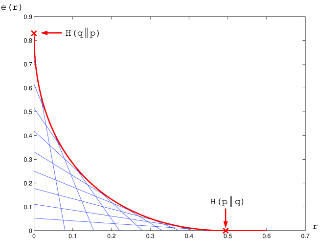
Figure 1: (Color online) Example plot of the error-exponent function $e(r)$, eq. (46), for the distributions $p=(0.95,0.05)$ and $q=(0.5,0.5)$. The thick (red) line is the graph of $e(r)$, while the thin (blue) lines are instances of the linear function $(-rs-\log\sum_{k}q_{k}^{s}p_{k}^{1-s})/(1-s)$ for various values of $s$, of which $e(r)$ is the point-wise maximum. For the chosen $p$ and $q$, the value of $H(p\|q)=0.49463$ and the value of $H(q\|p)=0.83037$.

Let $\phi=(\phi_{n})$ be a sequence of test functions. Recall the notations $\alpha_{R}(\phi)$ and $\beta_{R}(\phi)$ introduced in Section 2 for the rate limits (if they exist) of the corresponding type-I and type-II errors, respectively:

$$\alpha_{R}(\phi)=\lim_{n\rightarrow\infty}-\frac{1}{n}\log\alpha_{n}(\phi),\;\beta_{R}(\phi)=\lim_{n\rightarrow\infty}-\frac{1}{n}\log\beta_{n}(\phi)$$

Then the classical HBCL Theorem can be stated as follows.

Theorem 5.1

(HBCL) Assume that $p,q$ are mutually absolutely continuous. Then for each $r>0$ there exists a sequence $\phi$ of test functions $\phi_{n}$ such that the rate limits of the type-II and type-I errors behave like $\beta_{R}(\phi)\geq r$ and $\alpha_{R}(\phi)=e(r)$. Moreover, for any sequence $\phi$ such that $\alpha_{R}(\phi)$ and $\beta_{R}(\phi)$ both exist, the relation $\beta_{R}(\phi)>r$ implies $\alpha_{R}(\phi)\leq e(r)$.

We remark that for sequences $\phi$ of test functions $\phi_{n}$ for which the rate limits $\alpha_{R}(\phi)$ or $\beta_{R}(\phi)$ do not exist, the result still applies to subsequences $(\phi_{n_{k}})$ along which both error rate limits exist. The second part of the HBCL theorem is thus a statement about all accumulation points of $\left(-\frac{1}{n}\log\alpha_{n}(\phi),-\frac{1}{n}\log\beta_{n}(\phi)\right)$ for an arbitrary test sequence $\phi$.

Referring to Figure 1, the claim of this Theorem is that for any sequence of test functions $\phi$ the point $(\beta_{R}(\phi),\alpha_{R}(\phi))$ cannot be above the graph of $e(r)$ over $r>0$ and for any point on the graph over $r\geq 0$ one can find a sequence $\phi$. Since $\beta_{R}(\phi)=0$ may correspond to the case where $\beta(\phi_{n})$ vanishes subexponentially slowly as well as converges to a positive value, a rate limit of type-I error $\alpha_{R}(\phi)$ larger than $e(0)=H(q\|p)$ is achievable.

The case $\beta_{R}(\phi)>$ $r\geq H(p\|q)$, where $e(r)=0$, can be shown to correspond to $\alpha(\phi_{n})$ converging to $1$, rather than to $0$. (This is basically the content of the so-called ‘Strong Converse’.) In the case $\beta_{R}(\phi)=H(p\|q)$ a convergence of $\alpha(\phi_{n})$ to $0$ is achievable, albeit only subexponantially slowly (this is due to Stein’s Lemma.)

Note that in order to obtain a bound on $\beta_{R}$ under a constrained $\alpha_{R}$ one just has to interchange $p$ and $q$ in the Theorem.

5.2 Nonequivalent hypotheses

The Chernoff and Hoeffding bounds have typically been treated in the literature under a restrictive assumption that hypotheses $p,q$ are mutually absolutely continuous (equivalent), cf., e.g., Blahut blahut . As a prerequisite for a quantum generalisation, unless one wants to limit oneself to faithful states, one has to understand the classical Hoeffding bound for nonequivalent hypotheses. For the Chernoff bound, a corresponding discussion can be found in nussbaum without restrictions on the underlying sample space. Here we limit ourselves to finite sample spaces, thereby excluding infinite relative entropies for equivalent measures $p,q$.

For probability measures $p,q$ on a finite sample space $\Omega$, let $D_{0}$ be the support of $p$, $D_{1}$ be the support of $q$ and $B=$ $D_{0}\cap D_{1}$. Let $\psi_{0}=p\left(B\right)$, $\psi_{1}=q\left(B\right)$ and note that $\psi_{0}>0,\psi_{1}>0$ unless the measures $p,q$ are orthogonal (which we exclude for triviality). Define conditional measures given the set $B$: $\tilde{p}\left(\cdot\right)=p\left(\cdot|B\right)$, $\tilde{q}\left(\cdot\right)=q\left(\cdot|B\right)$. Note that $\tilde{p}$, $\tilde{q}$ are equivalent measures; we may have $\tilde{p}=\tilde{q}$. We consider hypothesis testing for a pair of product measures $p^{\otimes n},q^{\otimes n}$.

Recall that a (nonrandomised) test is a mapping $\phi_{n}:\Omega^{n}\mapsto\{0,1\}.$ In our setting, only observations in either $D_{0}^{n}$ or $D_{1}^{n}$ can occur, so we will modify the sample space to be $D_{0}^{n}\cup$ $D_{1}^{n}$. We will then establish relation of tests $\phi_{n}$ in the original problem $p^{\otimes n}$ vs. $q^{\otimes n}$ to tests in the ‘conditional’ problem $\tilde{p}^{\otimes n}$ vs. $\tilde{q}^{\otimes n},$ i.e. to tests $\tilde{\phi}_{n}$ $:B^{n}\mapsto\{0,1\}$. Call a test $\phi_{n}$ null admissible if it takes value $0$ on $D_{0}^{n}\setminus B^{n}$ and value $1$ on $D_{1}^{n}\setminus B^{n}$. These tests correspond to the notion that if a point in the sample space $\Omega^{n}$ is not in $B^{n}$, then it identifies the hypothesis errorfree (either $p$ or $q$). We need only consider null admissible tests; for any test there is a null admissible test with equal or smaller error probabilities $\alpha_{n}$, $\beta_{n}$. The restriction $\phi_{n}|B^{n}$ gives a test on $B^{n}$, i.e. in the conditional problem.

Lemma 3

There is a one-to-one correspondence between null admissible tests $\phi_{n}$ in the original problem $p^{\otimes n}$ vs. $q^{\otimes n}$ and tests $\tilde{\phi}_{n}$ in the conditional problem $\tilde{p}^{\otimes n}$ vs. $\tilde{q}^{\otimes n}$, given by $\tilde{\phi}_{n}=\phi_{n}|B^{n}$. The errror probabilities satisfy

$$\alpha_{n}\left(\phi\right)=\psi_{0}^{n}\alpha_{n}\left(\tilde{\phi}\right),\beta_{n}\left(\phi\right)=\psi_{1}^{n}\beta_{n}\left(\tilde{\phi}\right),$$

where $\psi_{0}=p(B)$ and $\psi_{1}=q(B)$.

Proof

The first claim is obvious, if one takes into account that we took all tests in the original problem to be mappings $\phi_{n}:D_{0}^{n}\cup$ $D_{1}^{n}\mapsto\{0,1\}$. For the relation of error probabilities, note that $p^{\otimes n}(A)=$ $\psi_{0}^{n}\tilde{p}^{\otimes n}(A\cap B^{n})$, $A\subset D_{0}^{n}\cup$ $D_{1}^{n}$ and therefore

$$\alpha_{n}\left(\phi\right) =\int\phi_{n}dp^{\otimes n}=\int_{B^{n}}\phi_{n}dp^{\otimes n}\text{ (by null admissibility)}$$

$$=\psi_{0}^{n}\int\phi_{n}d\tilde{p}^{\otimes n}=\psi_{0}^{n}\int_{B^{n}}\tilde{\phi}_{n}d\tilde{p}^{\otimes n}=\psi_{0}^{n}\alpha_{n}\left(\tilde{\phi}\right)$$

and analogously for $\beta_{n}\left(\phi\right).$ ∎

This result already allows to state the general Hoeffding bound in terms of the error-exponent function for the conditional problem

$$\tilde{e}(r)=\sup_{0\leq s<\ 1}\frac{-rs-\log\sum_{k}\tilde{q}_{k}^{s}\tilde{p}_{k}^{1-s}}{1-s}.$$

Indeed, rate limits $\alpha_{R}(\phi)$ and $\beta_{R}(\phi)$ for a null admissible test sequence $\phi$ exist if and only if they exist for the corresponding test sequence $\tilde{\phi}$, and

$$\alpha_{R}\left(\phi\right)=-\log\psi_{0}+\alpha_{R}\left(\tilde{\phi}\right)\text{, }\beta_{R}\left(\phi\right)=-\log\psi_{1}+\beta_{R}\left(\tilde{\phi}\right).$$ (47)

Proposition 3

Let $p,q$ be arbitrary probability measures on a finite sample space.
(i) (achievability) For each $r\geq-\log\psi_{1}$ there exists a sequence $\phi$ of test functions $\phi_{n}$ such that the rate limits of the type-II and type-I errors behave like $\beta_{R}\left(\phi\right)\geq r$ and $\alpha_{R}\left(\phi\right)=-\log\psi_{0}+\tilde{e}(r+\log\psi_{1})$. For the case $0\leq r\leq-\log\psi_{1}$, there is a sequence $\phi$ of test functions $\phi_{n}$ obeying $-n^{-1}\log\beta_{n}\left(\phi\right)=-\log\psi_{1}$ and $\alpha_{n}\left(\phi\right)=0$ for every $n.$
(ii) (optimality) Consider any sequence $\phi$ such that $\alpha_{R}(\phi)$ and $\beta_{R}(\phi)$ both exist. If $r\geq-\log\psi_{1}$ then the relation $\beta_{R}(\phi)>r$ implies $\alpha_{R}(\phi)\leq-\log\psi_{0}+\tilde{e}(r+\log\psi_{1})$.

Note that in (ii) the omission of the case $0\leq r\leq-\log\psi_{1}$ means that there is no upper bound on $\alpha_{R}(\phi),$ as shown by the achievability part ($\alpha_{R}\left(\phi\right)$ has to be set equal to $\infty$ for a test of vanishing error probability $\alpha_{n}$).

Proof

(i) Assume $r\geq-\log\psi_{1}$ and take a test sequence $\tilde{\phi}_{n}$ in the conditional problem $\tilde{p}^{\otimes n}$ vs. $\tilde{q}^{\otimes n}$ such that $\beta_{R}(\tilde{\phi})\geq r+\log\psi_{1}$ and $\alpha_{R}(\tilde{\phi})=\tilde{e}(r+\log\psi_{1})$, which exists according to the HBCL theorem since $\tilde{p},\tilde{q}$ are mutually absolutely continuous. According to Lemma 3, the corresponding null admissible test $\phi_{n}$ satisfies (47) and hence $\beta_{R}\left(\phi\right)\geq r$ and $\alpha_{R}\left(\phi\right)=-\log\psi_{0}+\tilde{e}(r+\log\psi_{1})$. Furthermore, consider the test $\tilde{\phi}_{n}\equiv 0$ in $\tilde{p}^{\otimes n}$ vs. $\tilde{q}^{\otimes n}$. This has $\alpha_{n}(\tilde{\phi}_{n})=0$ and $\beta_{n}(\tilde{\phi}_{n})=1$, hence the corresponding null admissible test $\phi_{n}$ has $\alpha_{n}(\phi_{n})=0$ and $\beta_{n}(\phi_{n})=\psi_{1}^{n}$.

(ii) Using a reduction to the conditional problem $\tilde{p}^{\otimes n}$ vs. $\tilde{q}^{\otimes n}$ similar to the one above, the optimality part also follows immediately from the HBCL theorem. ∎

Remark: Consider the dual of the test used in the second part of (i), i.e. the null admissible extension of the test $\tilde{\phi}_{n}\equiv 1$. This one obviously has $\alpha_{n}\left(\phi\right)=\psi_{0}^{n}$ and $\beta_{n}(\phi)=0$. It can be used for achievability for large $r$, i.e. it has $\beta_{R}(\phi)=\infty$ and $\alpha_{R}(\phi)=-\log\psi_{0}$.

It is possible to obtain a closed form expression for the Hoeffding bound, using the error-exponent function defined for $r\geq 0$ exactly as in (46), for the case of nonequivalent $p,q$. The difference is that we now have to admit a value $+\infty$ for certain arguments.

Lemma 4

For general $p,q$, the error-exponent function $e(r)$ satisfies

$$e(r)=\left\{\begin{array}[]{ll}-\log\psi_{0}+\tilde{e}(r+\log\psi_{1}),&\text{ for }r\leq-\log\psi_{1}\\ \infty,&\text{ for }0\leq r<-\log\psi_{1}.\end{array}\right.$$

Remark: For two distinct $p,q$ it is possible that $\tilde{p}=\tilde{q}$. In that case $\tilde{e}(r)=0$ for $r\geq 0$. It follows that $e(r)=\infty$ for $r<-log\psi_{1}$ and $e(r)=-\log\psi_{0}$ for $r\geq-\log\psi_{1}$. This case will be relevant in the quantum setting when the hypotheses will be represented by two non-orthogonal pure quantum states.

Proof

Assume $r\geq-\log\psi_{1}$ and set

$$e_{s}(r)=\frac{-rs-\log Q_{s}}{1-s}$$

where $Q_{s}=\sum_{k}p_{k}^{1-s}q_{k}^{s}$. Let $\tilde{Q}_{s}=\sum_{k}\tilde{p}_{k}^{1-s}\tilde{q}_{k}^{s}$ and note $Q_{s}=\psi_{0}^{1-s}\psi_{1}^{s}\tilde{Q}_{s}$. Hence

$$e_{s}(r) =\frac{-rs-(1-s)\log\psi_{0}-s\log\psi_{1}-\log\tilde{Q}_{s}}{1-s}$$

$$=-\log\psi_{0}+\frac{-(r+\log\psi_{1})s-\log\tilde{Q}_{s}}{1-s}=-\log\psi_{0}+\tilde{e}_{s}(r+\log\psi_{1})$$

where $\tilde{e}_{s}$ is the analogue of the function $e_{s}(r)$ with $Q_{s}$ replaced by $\tilde{Q}_{s}$. Since $e(r)=\sup_{0\leq s<\ 1}$ $e_{s}(r)$ and the analogue is true for $\tilde{e}_{s}$ and $\tilde{e}$, the claim follows in the case $r\geq-\log\psi_{1}$.

Assume now $0\leq r<-\log\psi_{1}$ and $\psi_{1}<1$, i.e.  $-\log\psi_{1}>0$. Clearly we have $Q_{s}\rightarrow\psi_{1}$ as $s\nearrow 1$, hence $-rs-\log Q_{s}\rightarrow-r-\log\psi_{1}>0$ as $s\nearrow 1$. Hence $\lim_{s\nearrow 1}e_{s}(r)=\infty$, and since $e(r)=\sup_{0\leq s<\ 1}$ $e_{s}(r)$, we also have $e(r)=\infty$. ∎

In conjunction with Proposition 3 we obtain a closed form description of the Hoeffding bound for possibly nonequivalent measures $p,q$, in terms of the original error-exponent function $e(r)$.

Theorem 5.2

Let $p,q$ be arbitrary probability measures on a finite sample space. Then the statement of the HBCL Theorem (Theorem 5.1) is true, where the error-exponent function defined in (46) obeys $e(r)=\infty$ for $0\leq r<-\log\psi_{1}$ if $\psi_{1}<1$.

We noted already that for $e(r)=\infty$, the bound on $\alpha_{R}(\phi)$ is achievable in the sense that a test exists having exactly $\alpha_{n}(\phi)=0$ for all $n$.

Using the properties of the rate function $\tilde{e}$ pertaining to equivalent measures $\tilde{p},\tilde{q}$, as illustrated in Figure 1, and the representation of Lemma 4 we obtain the following description of the general rate exponent function. In the interval $[0,-\log\psi_{1})$ it is infinity. At $r=$ $-\log\psi_{1}$ it takes value $e(r)=-\log\psi_{0}+H(\tilde{q}\|\tilde{p})=H(\tilde{q}\|p)$. For $r\geq-\log\psi_{1}$ it is convex and non-increasing. More precisely, over the interval $[-\log\psi_{1},-\log\psi_{1}+H(\tilde{p}\|\tilde{q})=H(\tilde{p}\|q)]$ $e(r)$ is convex (even strictly convex) and monotone decreasing. Over the interval $[H(\tilde{p}\|q),\infty)$ it is constant with value $-\log\psi_{0}$. A visual impression can be obtained by imagining the origin in Figure 1 shifted to the point $\left(-\log\psi_{1},-\log\psi_{0}\right)$. This picture will explicitly appear in Figure 2 below, in a situation further generalized to two quantum states with different supports.

5.3 Quantum Hoeffding Bound

In the quantum setting the error-exponent function $e(r)$ has to be replaced by a function $e_{Q}:{\mathbb{R}}^{+}_{0}\longrightarrow[0,\infty]$ given by

$$e_{Q}(r):=\sup_{0\leq s<1}\frac{-rs-\log\mathop{\rm Tr}\nolimits\sigma^{s}\rho^{1-s}}{1-s}.$$ (49)

In view of Proposition 1, $e_{Q}(r)$ coincides with the error-exponent function $e(r)$ for the pair of probability distributions $(p,q)$ associated with $(\rho,\sigma)$ via relation (12). Therefore, we can use Lemma 4 to describe properties of the function $e_{Q}(r)$, or the remarks after Theorem 5.2.

Recall that for a pair $(p,q)$, we defined a related pair of probability distributions $(\tilde{p},\tilde{q})$ by conditioning $p$ and $q$, respectively, on the intersection $B=D_{0}\cap D_{1}$ of the two support sets $D_{0}$ and $D_{1}$, and also $\psi_{0}=p(B),$ $\psi_{1}=q(B)$. In the present context, in accordance with (12) we have

$$D_{0}=\left\{(i,j):1\leq i,j\leq d,\;\lambda_{i}>0\right\},\;D_{1}=\left\{(i,j):1\leq i,j\leq d,\;\mu_{j}>0\right\}.$$

Let, as before, $\tilde{e}(r)$ be the error-exponent function pertaining to the pair $(\tilde{p},\tilde{q})$ according to (46). Then the quantum error-exponent function $e_{Q}(r)$ for the hypotheses $\rho,\sigma$ may be represented simply by

$$e_{Q}(r)=e(r)=\left\{\begin{array}[]{ll}-\log\psi_{0}+\tilde{e}(r+\log\psi_{1}),&\text{for }r\leq-\log\psi_{1}\\ \infty,&\text{for }0\leq r<-\log\psi_{1}.\end{array}\right.$$ (52)

It obtains its characteristic properties from the classical function being convex and monotone decreasing in the interval $\left[-\log\psi_{1},H(\tilde{p}\|q)\right]$ with $e(-\log\psi_{1})=H(\tilde{q}\|p)$, and constant with value $-\log\psi_{0}$ in the interval $[H(\tilde{p}\|q),\infty)$.

Lemma 5

Let supp $\rho$, supp $\sigma$ be the support projections associated with $\rho,\sigma$. Then the critical points and extremal values of $e_{Q}(r)$ may be expressed in a more direct way in terms of the density operators:

$$\psi_{0}=\mathrm{Tr}\left[\rho\;\mathrm{supp\ }\sigma\right],\quad\psi_{1}=\mathrm{Tr}\left[\sigma\;\mathrm{supp\ }\rho\right]$$

and

$$H(\tilde{p}\|q)=S_{\sigma}(\rho\|\sigma)\quad H(\tilde{q}\|p)=S_{\rho}(\sigma\|\rho),$$

where the entropy type quantities on the right-hand side are defined as

$$S_{\sigma}(\rho\|\sigma):=\mathrm{Tr}\left[\frac{\rho}{\psi_{0}}\;\left(\log\frac{\rho}{\psi_{0}}-\log\sigma\right)\mathrm{supp\ }\sigma\right],$$

$$S_{\rho}(\sigma\|\rho):=\mathrm{Tr}\left[\frac{\sigma}{\psi_{1}}\;\left(\log\frac{\sigma}{\psi_{1}}-\log\rho\right)\mathrm{supp\ }\rho\right].$$

Proof

Note that for $B=D_{0}\cap D_{1}$ we have

$$\psi_{0} =\sum_{(i,j)\in B}\lambda_{i}\left|\left\langle x_{i}|y_{j}\right\rangle\right|^{2}=\sum_{i,j}\lambda_{i}\;\mathrm{sgn}(\mu_{j})\;\left|\left\langle x_{i}|y_{j}\right\rangle\right|^{2}$$

$$=\sum_{i,j}\lambda_{i}\;\left|\left\langle x_{i}|\mathrm{sgn}(\mu_{j})y_{j}\right\rangle\right|^{2}=\sum_{i,j}\lambda_{i}\;\left|\left\langle x_{i}|\left(\mathrm{supp\ }\sigma\right)y_{j}\right\rangle\right|^{2}$$

$$=\sum_{i,j}\lambda_{i}\;\left|\left\langle\left(\mathrm{supp\ }\sigma\right)x_{i}|y_{j}\right\rangle\right|^{2}=\sum_{i}\lambda_{i}\;\left\|\left(\mathrm{supp\ }\sigma\right)x_{i}\right\|^{2}=$$

$$=\mathrm{Tr}\left[\sum_{i}\lambda_{i}\left|\left(\mathrm{supp\ }\sigma\right)x_{i}\right\rangle\left\langle\left(\mathrm{supp\ }\sigma\right)x_{i}\right|\right]=\mathrm{Tr}\left[\rho\;\mathrm{supp\ }\sigma\right]$$

and analogously for $\psi_{1}$. Furthermore

$$H(\tilde{p}\|q) =\sum_{(i,j)\in B}\tilde{p}_{i,j}\log\frac{\tilde{p}_{i,j}}{q_{i,j}}=\sum_{(i,j)\in B}\lambda_{i}\left|\left\langle x_{i}|y_{j}\right\rangle\right|^{2}\frac{1}{\psi_{0}}\log\frac{\lambda_{i}}{\mu_{j}\psi_{0}}$$

$$=\sum_{i,j}\mathrm{sgn}(\mu_{j})\left|\left\langle x_{i}|y_{j}\right\rangle\right|^{2}\frac{\lambda_{i}}{\psi_{0}}\log\frac{\lambda_{i}}{\psi_{0}}-\sum_{i,j}\mathrm{sgn}(\mu_{j})\left|\left\langle x_{i}|y_{j}\right\rangle\right|^{2}\frac{\lambda_{i}}{\psi_{0}}\log\mu_{j}$$

$$=\mathrm{Tr}\left[\frac{\sigma}{\psi_{1}}\;\left(\log\frac{\sigma}{\psi_{1}}\right)\mathrm{supp\ }\rho\right]-\mathrm{Tr}\left[\frac{\sigma}{\psi_{1}}\;\left(\log\rho\right)\mathrm{supp\ }\rho\right]$$

where the third equality is analogous to the calculation in the proof of Proposition 1. ∎

To shed some light on the entropy type quantity $S_{\sigma}(\rho\|\sigma)$, note that it may be rewritten as a difference of usual (Umegaki’s) relative entropies:

$$S_{\sigma}(\rho\|\sigma)=S(\frac{\rho}{\psi_{0}}\textrm{supp }\sigma\|\sigma)-S(\frac{\rho}{\psi_{0}}\textrm{supp }\sigma\|\frac{\rho}{\psi_{0}}).$$

This may be verified by direct calculations similar to those in the proof of Lemma 5.

The linear operator $\frac{\rho}{\psi_{0}}\textrm{supp }\sigma$ is a kind of conditional expectation of $\rho$. While it is not self-adjoint, the relative entropies on the right-hand side are well defined (in a mathematical sense) and real: first, the entropy of $\frac{\rho}{\psi_{0}}\textrm{supp }\sigma$ is defined in terms of its spectrum, which is positive and normalised to 1, hence giving a real, positive entropy, and second, $\mathop{\rm Tr}\nolimits[\rho\,\,\textrm{supp }\sigma\log(\rho)]$ can be written as $\mathop{\rm Tr}\nolimits[\textrm{supp }\sigma\rho\log\rho\,\,\textrm{supp }\sigma]$, from which it is evident that this term is also real.

It is easily seen from the above formula that $S_{\sigma}(\rho\|\sigma)$ coincides with $S(\rho\|\sigma)$ if $\sigma$ is a faithful state, or more generally if $\mathrm{supp\ }\rho\leq\mathrm{supp\ }\sigma$. Otherwise $S(\rho\|\sigma)=\infty$, while $S_{\sigma}(\rho\|\sigma)$ is finite.

Note also that $S_{\rho}(\sigma\|\rho)\geq-\log\psi_{0}$ and equality holds if and only if it holds in $S_{\sigma}(\rho\|\sigma)\geq-\log\psi_{1}$. This immediately follows from $S_{\rho}(\sigma\|\rho)+\log\psi_{0}=$ $H(\tilde{p}\|\tilde{q})$, which is seen from Lemma 5. This happens in particular if both $\rho$ and $\sigma$ are pure states. In this case there is only one pair $(i,j)$ where both $\lambda_{i}>0$ and $\mu_{j}>0$, hence the set $B$ consists of one element only. In this case we must have $\tilde{p}=\tilde{q},$ hence $H(\tilde{p}\|\tilde{q})=H(\tilde{q}\|\tilde{p})=0$.

The general shape of the quantum error-exponent function $e_{Q}(r)$ is represented in Figure 2. If both $\rho$ and $\sigma$ are pure states then the shape degenerates to ‘rectangular’ form ($e_{Q}(r)=\infty$ or $e_{Q}(r)=-\log\psi_{1}$).

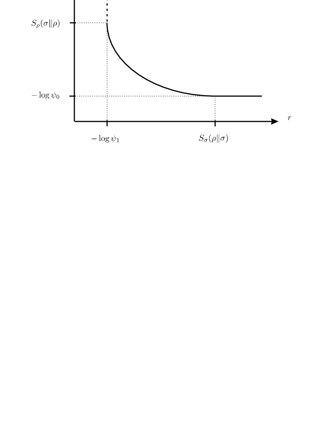
Figure 2: Example plot of the quantum error-exponent function $e_{Q}(r)$ in the general case.

A quantum generalisation of the HBCL Theorem then reads as follows.

Theorem 5.3

(Quantum HBCL)For each $r>0$ there exists a sequence $\Pi$ of test projections $\Pi_{n}$ on $\mathcal{H}^{\otimes n}$ for which the rate limits of type-I and type-II errors behave like $\alpha_{R}(\Pi)=e_{Q}(r)$ and $\beta_{R}(\Pi)\geq r$, respectively. Moreover, for any sequence $\Pi$ such that $\alpha_{R}(\Pi)$ and $\beta_{R}(\Pi)$ both exist, the relation $\beta_{R}(\Pi)>r$ implies $\alpha_{R}(\Pi)\leq e_{Q}(r)$.

The statement of the quantum HBCL Theorem is that for every sequence $\Pi$ (for which both error rate limits exist) the point $(\beta_{R}(\Pi),\alpha_{R}(\Pi))$ lies on or below the curve $e_{Q}(r)$ over $(0,\infty]$, and for every point on the curve over the closed interval $[0,\infty]$ there is a sequence $\Pi$ achieving it.

We remark that, just like (41), the relationship (45) seems to have no general quantum counterpart, even when both states are faithful. In other words, there is no known subset of linear operators $\tau$ with positive spectrum such that $e_{Q}(r)=\inf_{\tau}\{S(\tau\|\rho):S(\tau\|\sigma)\leq r\}$.

To prove the quantum Hoeffding bound, the following lemmas are needed.

Lemma 6

For scalars $x,y>0$, bounds on $\log(x+y)$ are given by

$$\max(\log x,\log y)\leq\log(x+y)\leq\max(\log x,\log y)+\log 2.$$ (53)

Proof. For the first inequality, put $x=e^{a}$ and $y=e^{b}$, and note

$$\log(e^{a}+e^{b}) = a+\log(1+e^{b-a})$$

$$\geq a+\max(0,b-a)$$

$$= \max(a,b).$$

The second inequality follows directly from the fact that the logarithm increases monotonically, so that $\log((x+y)/2)\leq\log\max(x,y)$. ∎

A direct consequence of this Lemma is

Lemma 7

For two scalar sequences $x_{n},y_{n}>0$ with rate limits $x_{R}$ and $y_{R}$, the rate limit of $x_{n}+y_{n}$ is given by

$$\lim_{n\to\infty}-\frac{1}{n}\log(x_{n}+y_{n})=\min(x_{R},y_{R}).$$ (54)

5.4 Proof of Optimality of the Quantum Hoeffding Bound

Again we use the mapping from the pair $(\rho,\sigma)$ to the pair $(p,q)$, so that, by Proposition 1, $e(r)=e_{Q}(r)$. From Proposition 2 we have that for any sequence $\Pi$ of orthogonal projections $\Pi_{n}$ and for any real value of the scalar $x$, for all $n\in\mathbb{N}$ one as

$$\alpha(\Pi_{n})+e^{-nx}\beta(\Pi_{n})\geq\frac{1}{2}\left(\alpha(\phi_{n})+e^{-nx}\beta(\phi_{n})\right),$$

where $\phi_{n}$ are classical test functions corresponding to the maximum likelihood decision rule, cf. the proof of Proposition 2. Recall that the type-I and type-II errors are defined as $\alpha(\phi_{n})=\sum_{i}p_{i}^{n}\phi_{n}(i)$ and $\beta(\phi_{n})=\sum_{i}q_{i}^{n}(1-\phi_{n}(i)).$

On taking the rate limit on the left side, this gives

$$\lim_{n\rightarrow\infty}-\frac{1}{n}\log\left(\alpha(\Pi_{n})+e^{-nx}\beta(\Pi_{n})\right)\leq\liminf_{n\rightarrow\infty}-\frac{1}{n}\log\left(\alpha(\phi_{n})+e^{-nx}\beta(\phi_{n})\right)$$

By possibly taking a subsequence, we can ensure that the rate limits $\alpha_{R}(\phi)$, $\beta(\phi_{n})$ also exist. By Lemma 7, the above simplifies to

$$\min(\alpha_{R}(\Pi),x+\beta_{R}(\Pi))\leq\min(\alpha_{R}(\phi),x+\beta_{R}(\phi)).$$ (55)

Assume now that $\beta_{R}(\phi)\leq-\log\psi_{1}$. Then, by selecting $x<0$ and $\left|x\right|$ sufficiently large, we obtain $x+\beta_{R}(\Pi)\leq x+\beta_{R}(\phi)$ and hence $\beta_{R}(\Pi)\leq-\log\psi_{1}$. Since $e_{Q}(r)=\infty$ for $r<\beta_{R}(\Pi)\leq-\log\psi_{1}$ according to the discussion above Lemma 5, the claim $\alpha_{R}(\Pi)\leq e_{Q}(r)$ holds trivially. Henceforth we assume that $\beta_{R}(\phi)>-\log\psi_{1}$.

From the classical HBCL Theorem (more precisely, from Theorem 5.2), the right-hand side of (55) is bounded above by $\min(e(r),x+\beta_{R}(\phi))$, for any $r$ with $-\log\psi_{1}\leq r<\beta_{R}(\phi)$. Note that $e(r)$ is continuous for $r\geq-\log\psi_{1}$ (since it is monotonely nonincreasing and convex). By letting $r\nearrow\beta_{R}(\phi)$ we obtain an upper bound $\min(e(r),x+r)$ with $r\geq-\log\psi_{1}$.

We can now prove the optimality part of the quantum HBCL Theorem, using only this upper bound plus the fact that $e(r)$ is monotonously decreasing.

The upper bound $\min(e(r),x+r)$ holds for some particular value $r$. We will find a further upper bound by maximizing over $r\geq-\log\psi_{1}$. For this we have to distinguish two cases, depending on the value of $x.$

a) At $r=-\log\psi_{1}$ we have $e(r)>x+r$. Since $e(r)$ is decreasing in $r$ and continuous, and $x+r$ is increasing, the maximum of $\min(e(r),x+r)$ is obtained when $e(r)=x+r$. Let $r^{\ast}(x)>-\log\psi_{1}$ be the solution of $x+r=e(r)$. We now have that for any sequence of quantum measurements $\Pi$ and for any real value of the scalar $x$,

$$\min(\alpha_{R}(\Pi),x+\beta_{R}(\Pi))\leq x+r^{\ast}(x)=e(r^{\ast}(x)).$$

b) At $r=-\log\psi_{1}$ we have $e(r)\leq x+r$. Again by the properties of $e(r)$ and $x+r$, the maximum of $\min(e(r),x+r)$ is $e(r^{\ast})$ is attained for $r^{\ast}(x)=-\log\psi_{1}$. We then obtain the upper bound

$$\min(\alpha_{R}(\Pi),x+\beta_{R}(\Pi))\leq e(r^{\ast}(x)).$$

Now set $x=\alpha_{R}(\Pi)-\beta_{R}(\Pi)$, then both inequalities above yield $\alpha_{R}(\Pi)\leq e(r^{\ast})$. Assume $r<\beta_{R}(\Pi)$; we intend to show that this implies $\alpha_{R}(\Pi)\leq e(r)$. Indeed, in both cases a) and b) $r^{\ast}$ is such that

$$e(r^{\ast})\leq x+r^{\ast}=\alpha_{R}(\Pi)-\beta_{R}(\Pi)+r^{\ast}<\alpha_{R}(\Pi)-r+r^{\ast}$$

hence $r^{\ast}-r\geq e(r^{\ast})-\alpha_{R}(\Pi)\geq 0$. Therefore, from the monotonicity of the error-exponent function follows $e(r^{\ast})\leq e(r)$ and we finally obtain $\alpha_{R}(\Pi)\leq e(r)=e_{Q}(r)$. ∎

5.5 Proof of Achievability of the Quantum Hoeffding Bound

The proof of achievability is mainly due to Hayashi hayashi06 , who used inequality (28), which is obtained as a byproduct of the proof of Theorem 3.2. However, we modify it avoiding any implicit assumption that the involved quantum states are faithful; hence we prove Theorem 5.3 in full generality, which includes for example the case of two non-orthogonal pure states.

Let us fix an arbitrary $s\in(0,1)$, and set

$$a = e^{-nx}\sigma^{\otimes n}$$ (56)

$$b = \rho^{\otimes n},$$ (57)

where the value of $x$ will be chosen in due course. Consider the sequence of POVMs $\{(\mathrm{\leavevmode\hbox{\small 1\normalsize\kern-3.30002pt1}}-\Pi_{n},\Pi_{n})\}$ with $\Pi_{n}$ the projector on the range of $(a-b)_{+}$; again element $\mathrm{\leavevmode\hbox{\small 1\normalsize\kern-3.30002pt1}}-\Pi_{n}$ is assigned to the null hypothesis $\rho^{\otimes n}$, and element $\Pi_{n}$ is assigned to the alternative hypothesis $\sigma^{\otimes n}$. We will show that this POVM asymptotically attains the Hoeffding bound.

Recall that inequality (28) states

$$\mathop{\rm Tr}\nolimits[a^{s}b^{1-s}]\geq\mathop{\rm Tr}\nolimits[\Pi b+(\mathrm{\leavevmode\hbox{\small 1\normalsize\kern-3.30002pt1}}-\Pi)a].$$

By positivity of $\mathop{\rm Tr}\nolimits[\Pi b]$ and $\mathop{\rm Tr}\nolimits[(\mathrm{\leavevmode\hbox{\small 1\normalsize\kern-3.30002pt1}}-\Pi)a]$, this implies the two inequalities

$$\mathop{\rm Tr}\nolimits[\Pi b],\mathop{\rm Tr}\nolimits[(\mathrm{\leavevmode\hbox{\small 1\normalsize\kern-3.30002pt1}}-\Pi)a]\leq\mathop{\rm Tr}\nolimits[a^{s}b^{1-s}].$$

These yield the following upper bounds on the $\alpha$ and $\beta$ errors of the chosen POVM (recall $Q_{s}=\mathop{\rm Tr}\nolimits[\rho^{1-s}\sigma^{s}]$):

$$\beta_{n}(\Pi_{n}) = \mathop{\rm Tr}\nolimits[(\mathrm{\leavevmode\hbox{\small 1\normalsize\kern-3.30002pt1}}-\Pi_{n})\sigma^{\otimes n}]$$ (58)

$$= e^{nx}\mathop{\rm Tr}\nolimits[(\mathrm{\leavevmode\hbox{\small 1\normalsize\kern-3.30002pt1}}-\Pi_{n})a]$$

$$\leq e^{nx}\mathop{\rm Tr}\nolimits[a^{s}b^{1-s}]$$

$$= e^{nx(1-s)}Q_{s}^{n}$$

$$= \exp[n(x(1-s)+\log Q_{s})].$$

$$\alpha_{n}(\Pi_{n}) = \mathop{\rm Tr}\nolimits[\Pi_{n}\rho^{\otimes n}]$$ (59)

$$= \mathop{\rm Tr}\nolimits[\Pi_{n}b]$$

$$\leq \mathop{\rm Tr}\nolimits[a^{s}b^{1-s}]$$

$$= e^{-nxs}Q_{s}^{n}$$

$$= \exp[n(-xs+\log Q_{s})].$$

Choosing $x$ such that $x(1-s)+\log Q_{s}=-r$ then yields, from (58),

$$\beta_{n}(\Pi_{n}) \leq \exp(-nr),$$

and from (59),

$$\alpha_{n}(\Pi_{n}) \leq \exp\left(-n\left(-s\frac{r+\log Q_{s}}{1-s}-\log Q_{s}\right)\right)$$

$$= \exp\left(-n\frac{-rs-\log Q_{s}}{1-s}\right)$$

$$\leq \exp\left(-ne_{Q}\left(r\right)\right),$$

where in the last inequality we have used the fact that the parameter $s$ was arbitrarily chosen from $(0,1)$.

Thus, for the rate limits we get

$$\beta_{R}\geq r,\quad\alpha_{R}\geq e_{Q}(r).$$

The optimality, proven in the previous subsection, states that $\alpha_{R}\leq e_{Q}(r)$ if $\beta_{R}=r$. Furthermore, since $e_{Q}(r)$ is a non-increasing function, $\alpha_{R}\leq e_{Q}(r)$ if $\beta_{R}>r$. This implies that for the chosen sequence of POVMs

$$\beta_{R}=r,\quad\alpha_{R}=e_{Q}(r)$$

must hold, which proves that the Hoeffding bound is indeed attained. ∎

5.6 Quantum Stein’s Lemma and quantum version of Sanov’s Theorem

The quantum generalisation of Stein’s lemma deals with the asymptotics of the error quantity

$$\beta_{n}^{*}(\epsilon):=\inf_{\Pi_{n}}\{\beta_{n}(\Pi_{n}):\alpha_{n}(\Pi_{n})\leq\epsilon\},$$ (60)

for fixed $0<\epsilon<1$. Here, the infimum is taken over all positive semi-definite contractions $\Pi_{n}$ on $\mathcal{H}^{\otimes n}$.

Quantum Stein’s Lemma states that the rate limit $\beta_{R}^{*}(\varepsilon)$ of the sequence $(\beta_{n}^{*}(\epsilon))$ exists and is equal to $S(\rho\|\sigma)$, independently of $\epsilon$. It was first obtained by Hiai and Petz hiaipetz . Its optimality part was then strengthened by Ogawa and Nagaoka in ogawa .

Here we use the quantum HBCL Theorem to prove that the relative entropy $S(\rho\|\sigma)$ is an achievable error rate limit and deduce optimality of this bound from Proposition 1 in qSanov2 .

Proof of the quantum Stein’s lemma. We need to show that there is a sequence $\Pi$ with $\alpha(\Pi_{n})\leq\epsilon$ achieving $\beta_{R}(\Pi)=S(\rho\|\sigma)$. Let $\eta>0$ be small and set $r=S(\rho||\sigma)-\eta$. Achievability of the quantum Hoeffding bound means that a sequence $\Pi$ exists for which $\beta_{R}\geq r$ and $\alpha_{R}=e_{Q}(r)$. Since $e_{Q}(r)>0$ for all $r<S(\rho\|\sigma)$ and $\eta>0$, the sequence $\alpha_{n}$ converges to 0. Thus, from a certain value of $n$ onwards, $\alpha_{n}$ will get lower than any value $\epsilon>0$ chosen beforehand. This means that $\Pi$ is a feasible sequence in (60) for $n$ large enough, exhibiting $\beta_{R}(\epsilon)\geq r=S(\rho\|\sigma)-\eta$. As this holds for any $\eta>0$, we find that $\beta_{R}^{*}(\epsilon)\geq S(\rho\|\sigma)$.

With $\beta_{R}^{*}(\epsilon)\geq S(\rho\|\sigma)$ the two hypotheses associated to the pair of density operators $(\rho,\sigma)$ satisfy the HP-condition in the terminology of the paper qSanov2 . Thus Proposition 1 in qSanov2 implies $\beta_{R}^{*}(\epsilon)=S(\rho\|\sigma)$.

∎

We remark that in qSanov2 the HP-condition was introduced for (ordered) pairs $(\Psi,\Phi)$ of arbitrary correlated states on quantum spin chains, while in the present paper only density operators of the tensor-product form $\rho^{\otimes n}$ have been considered. These correspond to the special case of shift-invariant product states on the infinite spin chain (quantum i.i.d. states). A pair $(\Psi,\Phi)$ is said to satisfy the HP-condition if the relative entropy rate $s(\Psi\|\Phi)$ exists and is a lower bound on the lower rate limit $\underline{\beta}_{R}^{*}(\varepsilon)$ for all $\varepsilon\in(0,1)$.

Specifically to our setting (the i.i.d. case), Theorem 1 in qSanov2 states that the achievability part in quantum Stein’s Lemma (the HP-condition) is equivalent to a quantum version of Sanov’s theorem, which has been presented in qSanov and which is a priori a result extending quantum Stein’s Lemma in the following way:

Let the null hypothesis $H_{0}$ correspond to a family $\Gamma$ of density operators on $\mathcal{H}$ instead of a single density operator $\rho$. Let the alternative hypothesis $H_{1}$ be still represented by a fixed density operator $\sigma$. Then there exists a sequence $\Pi$ of orthogonal projections $\Pi_{n}$ on $\mathcal{H}^{\otimes n}$, respectively, such that for all $\rho\in\Gamma$ the corresponding type-I error vanishes asymptotically, i.e.

$$\lim_{n\to\infty}\mathop{\rm Tr}\nolimits[\rho^{\otimes n}\Pi_{n}]=0,$$ (61)

while the type-II error rate limit $\beta_{R}(\Pi)$ is equal to the relative entropy distance from $\Gamma$ to $\sigma$:

$$S(\Gamma\|\sigma):=\inf_{\rho\in\Gamma}S(\rho\|\sigma).$$

Moreover $S(\Gamma\|\sigma)$ is the upper bound on type-II error (upper) rate limit, for any sequence $\Pi$ of POVMs satisfying the constraint (61).

With the above reasoning we obtain the statement of quantum Sanov’s Theorem from the quantum HBCL Theorem as well.

6 Acknowledgements

We thank the hospitality of various institutions: the Max Planck Institute for Quantum Optics (FV, KA), the Erwin Schrödinger Institute in Vienna (FV, KA, AS), and the Physics Department of the National University of Singapore (KA). KA was supported by The Leverhulme Trust (grant F/07 058/U), by the QIP-IRC (www.qipirc.org) supported by EPSRC (GR/S82176/0), by EU Integrated Project QAP, and by the Institute of Mathematical Physics, Imperial College London. MN has been supported by NSF under grant DMS-03-06497.

Appendix A Proofs of Bounds on $Q$

Inequality (36) stated in terms of general positive operators is

Theorem A.1

For positive operators $A$ and $B$, and $0\leq s\leq 1$,

$$\|A^{1/2}B^{1/2}\|_{1}\leq(\mathop{\rm Tr}\nolimits[A^{s}B^{(1-s)}])^{1/2}\,(\mathop{\rm Tr}\nolimits[A])^{(1-s)/2}\,(\mathop{\rm Tr}\nolimits[B])^{s/2}.$$ (62)

Specialising to states, $A=\sigma$ and $B=\rho$, the left-hand side is just $F(\rho,\sigma)$, while the right-hand side is equal to $Q_{s}(\rho,\sigma)^{1/2}$.

Proof. We rewrite $A^{1/2}B^{1/2}$ as a product of three factors

$$A^{1/2}B^{1/2}=A^{(1-s)/2}(A^{s/2}B^{(1-s)/2})B^{s/2},$$

apply Hölder’s inequality on the 1-norm of this product, and exploit the relation

$$\|X^{p}\|_{q}=\|X\|^{p}_{pq}$$

(for $X\geq 0$) a number of times.

$$\|A^{1/2}B^{1/2}\|_{1} = \|A^{(1-s)/2}(A^{s/2}B^{(1-s)/2})B^{s/2}\|_{1}$$

$$\leq \|A^{(1-s)/2}\|_{2/(1-s)}\,\|A^{s/2}B^{(1-s)/2}\|_{2}\,\|B^{s/2}\|_{2/s}$$

$$= (\mathop{\rm Tr}\nolimits[A])^{(1-s)/2}\,\|A^{s/2}B^{(1-s)/2}\|_{2}\,(\mathop{\rm Tr}\nolimits[B])^{s/2}$$

$$= (\mathop{\rm Tr}\nolimits[A^{s}B^{(1-s)}])^{1/2}\,(\mathop{\rm Tr}\nolimits[A])^{(1-s)/2}(\mathop{\rm Tr}\nolimits[B])^{s/2}.$$

∎

We now give a direct proof of inequality (34) that circumvents the proof of (33) and goes through in infinite dimensions. We state it in terms of general positive operators:

Theorem A.2

For positive operators $A$ and $B$,

$$\|A-B\|_{1}^{2}+4(\mathop{\rm Tr}\nolimits[A^{1/2}B^{1/2}])^{2}\leq(\mathop{\rm Tr}\nolimits(A+B))^{2}.$$ (63)

Proof. Consider two general operators $P$ and $Q$, and define their sum and difference as $S=P+Q$ and $D=P-Q$. We thus have $P=(S+D)/2$ and $Q=(S-D)/2$. Consider the quantity

$$PP^{*}-QQ^{*} = \frac{1}{4}\left((S+D)(S+D)^{*}-(S-D)(S-D)^{*}\right)$$

$$= \frac{1}{2}(SD^{*}+DS^{*}).$$

Its trace norm is bounded above as

$$\|SD^{*}+DS^{*}\|_{1}/2 \leq (\|SD^{*}\|_{1}+\|DS^{*}\|_{1})/2$$

$$= \|SD^{*}\|_{1}$$

$$\leq \|S\|_{2}\|D\|_{2}.$$

In the last line we have used a specific instance of Hölder’s inequality for the trace norm (bhatia Cor. IV.2.6). Now put $P=A^{1/2}$ and $Q=B^{1/2}$, which exist by positivity of $A$ and $B$, and which are themselves positive operators. We get $S,D=A^{1/2}\pm B^{1/2}$, hence

$$\|A-B\|_{1}\leq\|A^{1/2}+B^{1/2}\|_{2}\,\,\|A^{1/2}-B^{1/2}\|_{2},$$

which upon squaring becomes

$$\|A-B\|_{1}^{2} \leq \mathop{\rm Tr}\nolimits(A^{1/2}+B^{1/2})^{2}\,\,\mathop{\rm Tr}\nolimits(A^{1/2}-B^{1/2})^{2}$$

$$= \mathop{\rm Tr}\nolimits(A+B+A^{1/2}B^{1/2}+B^{1/2}A^{1/2})$$

$$\times\mathop{\rm Tr}\nolimits(A+B-A^{1/2}B^{1/2}-B^{1/2}A^{1/2})$$

$$= (\mathop{\rm Tr}\nolimits(A+B)+2\mathop{\rm Tr}\nolimits(A^{1/2}B^{1/2}))$$

$$\times(\mathop{\rm Tr}\nolimits(A+B)-2\mathop{\rm Tr}\nolimits(A^{1/2}B^{1/2}))$$

$$= (\mathop{\rm Tr}\nolimits(A+B))^{2}-4(\mathop{\rm Tr}\nolimits(A^{1/2}B^{1/2}))^{2}.$$

∎

References

- (1) K.M.R. Audenaert, J. Calsamiglia, R. Munoz-Tapia, E. Bagan, Ll. Masanes, A. Acin and F. Verstraete, “Discriminating States: The Quantum Chernoff Bound”, Phys. Rev. Lett. 98, 160501 (2007).
- (2) D. Bacon, I. Chuang, A. Harrow, “Efficient Quantum Circuits for Schur and Clebsch-Gordan Transforms”, arxiv.org E-print quant-ph/0407082.
- (3) R. Bhatia, Matrix Analysis, Springer, Heidelberg (1997).
- (4) I. Bjelaković, J.D. Deuschel, T. Krüger, R. Seiler, Ra. Siegmund-Schultze, A. Szkoła, “A quantum version of Sanov’s theorem”, Comm. Math. Phys. 260, 659-671 (2005).
- (5) I. Bjelaković, J.D. Deuschel, T. Krüger, R. Seiler, Ra. Siegmund-Schultze, A. Szkoła, “Typical support and Sanov large deviation of correlated states”, arXiv.org E-print math/0703772.
- (6) R.E. Blahut, “Hypothesis Testing and Information Theory”, IEEE Trans. Inf. Theory 20, 405–417 (1974).
- (7) E.A. Carlen and E.H. Lieb, Advances in Math. Sciences, AMS Transl. (2) 189, 59–62 (1999). See also arxiv.org E-print math.OA/0701352.
- (8) H. Chernoff, “A Measure of Asymptotic Efficiency for Tests of a Hypothesis based on the Sum of Observations”, Ann. Math. Stat. 23, 493–507 (1952).
- (9) I. Csiszár and G. Longo, Studia Sci. Math. Hungarica 6, 181–191 (1971).
- (10) C.A. Fuchs and J. van de Graaf, “Cryptographic distinguishability measures for quantum-mechanical states”, IEEE Trans. Inf. Theory 45, 1216 (1999).
- (11) M. Hayashi, Quantum Information, An Introduction, Springer, Berlin (2006).
- (12) M. Hayashi, “Error Exponent in Asymmetric Quantum Hypothesis Testing and Its Application to Classical-Quantum Channel coding”, arxiv.org E-print quant-ph/0611013 (2006).
- (13) M. Hayashi, “Asymptotics of quantum relative entropy from a representation theoretical viewpoint”, J. Phys. A: Math. Gen. 34, 3413-3419 (2001)
- (14) C.W. Helstrom, Quantum Detection and Estimation Theory, Academic Press, New York (1976).
- (15) F. Hiai and D. Petz, “The proper formula for relative entropy and its asymptotics in quantum probability”, Commun. Math. Phys. 143, 99–114 (1991).
- (16) W. Hoeffding, “Asymptotically Optimal Tests for Multinomial Distributions”, Ann. Math. Statist. 36, 369–401 (1965).
- (17) A.S. Holevo, “On Asymptotically Optimal Hypothesis Testing in Quantum Statistics”, Theor. Prob. Appl. 23, 411–415 (1978).
- (18) V. Kargin, “On the Chernoff distance for efficiency of quantum hypothesis testing,” Ann. Statist. 33, 959–976 (2005).
- (19) E.H. Lieb, “Convex trace functions and the Wigner-Yanase-Dyson conjecture”, Adv. Math. 11, 267–288 (1973).
- (20) H. Nagaoka, “The Converse Part of The Theorem for Quantum Hoeffding Bound”, arxiv.org E-print quant-ph/0611289 (2006).
- (21) M. Nussbaum and A. Szkoła, “A lower bound of Chernoff type in quantum hypothesis testing”, arxiv.org E-print quant-ph/0607216 (2006).
- (22) M. Nussbaum and A. Szkoła, “The Chernoff lower bound in quantum hypothesis testing”, Preprint No. 69/2006, MPI MiS Leipzig.
- (23) T. Ogawa and M. Hayashi, “On error exponents in quantum hypothesis testing”, IEEE Trans. Inf. Theory 50, 1368–1372 (2004).
- (24) T. Ogawa and H. Nagaoka, “Strong converse and Stein’s lemma in quantum hypothesis testing”, IEEE Trans. Inf. Theory 46, 2428 (2000).
- (25) A.W. van der Vaart, Asymptotic Statistics, Cambridge University Press (1998).
- (26) A. Uhlmann, “Sätze über Dichtematrizen”, Wiss. Z. Karl-Marx Univ. Leipzig 20, 633–653 (1971).
- (27) A. Uhlmann, “The ‘transition probability’ in the state space of a *-algebra”, Rep. Math. Phys. 9, 273 (1976).