Soft-pulse dynamical decoupling in a cavity

Abstract

Dynamical decoupling is a coherent control technique where the intrinsic and extrinsic couplings of a quantum system are effectively averaged out by application of specially designed driving fields (refocusing pulse sequences). This entails pumping energy into the system, which can be especially dangerous when it has sharp spectral features like a cavity mode close to resonance. In this work we show that such an effect can be avoided with properly constructed refocusing sequences. To this end we construct the average Hamiltonian expansion for the system evolution operator associated with a single “soft” $\pi$-pulse. To second order in the pulse duration, we characterize a symmetric pulse shape by three parameters, two of which can be turned to zero by shaping. We express the effective Hamiltonians for several pulse sequences in terms of these parameters, and use the results to analyze the structure of error operators for controlled Jaynes-Cummings Hamiltonian. When errors are cancelled to second order, numerical simulations show excellent qubit fidelity with strongly-suppressed oscillator heating.

I Introduction

Quantum coherent control has found way into many applications, including nuclear magnetic resonance (NMR), quantum information processing (QIP), spintronics, atomic physics, etc. The simplest control technique is dynamical decoupling (DD), also known as refocusing. The goal of preserving coherence by averaging out the unwanted couplings is achieved most readily by running precisely designed sequences of uniformly-shaped pulses Slichter (1992); Freeman (1998); Vandersypen and Chuang (2004).

In a closed system, the corresponding performance can be analyzed in terms of the average Hamiltonian theoryWaugh et al. (1968a, b). To leading order, the evolution over the refocusing period $\tau$ is indeed described by the time-averaged Hamiltonian of the system in the “rotating frame” defined by the control fields. Generally, the average Hamiltonian is constructed as a series in powers of $\tau$. The number of the leading terms of this expansion that are exactly zero determines the order $K$ of the refocusing sequence. Larger $K$ imply asymptotically more accurate refocusing, with error terms scaling to zero faster with decreasing $\tau$.

For an open system, the dynamics associated with the bath degrees of freedom can be also averaged out, as long as they are sufficiently slow. With leading-order ($K=1$) refocusing, the state decay processes are dramatically suppressedKofman and Kurizki (2001, 2004), with a moderate decrease of the dephasing ratePryadko and Sengupta (2006), while with second-order refocusing ($K=2$) both decay and dephasing are strongly suppressedPryadko and Sengupta (2006).

The decoherence analysis in Ref. Pryadko and Sengupta (2006) was based on the assumption of the low-frequency oscillator bath being near thermal equilibrium. This assumption becomes questionable if the bath has sharp spectral features—e.g., if the controlled qubit system is coupled to a local high-$Q$ oscillator. On the other hand, such a situation where the controlled system is coupled to an oscillator mode is quite common. This situation is realized in atomic physics, where the oscillator in question is the cavity mode, while the continuous-wave (CW) excitation is used to suppress the couplingVillas-Boas et al. (2004). In several quantum computer designs, nearly-linear oscillator modes are inherently present (e.g., mutual displacement in ion trapsCirac and Zoller (1995); Vitali and Tombesi (1999); You (2001); Kielpinski et al. (2002); Vitali and Tombesi (2002), or QCs based on electrons on heliumPlatzman and Dykman (1999); Dykman and Platzman (2000); Lea et al. (2000); Dykman et al. ). Finally, there are suggestions to include local high-$Q$ oscillators in the QC designs to serve as “quantum memory” Pritchett and Geller (2005), “quantum information bus”Kapale et al. (2005); Wei et al. (2005); Geller and Cleland (2005), or as a part of the measuring/control circuitryBlais et al. (2007).

In this work we consider dynamical decoupling in a system where the spectral function of the oscillator bath has a sharp resonance. We include the resonant mode and the corresponding couplings in the system Hamiltonian, and consider the dynamics of the closed system driven by the refocusing pulses applied to the qubits only. We construct the average Hamiltonian for a situation where one of the qubits is driven by a single symmetrical one-dimensional $\pi$-pulse. To second order, the expansion is characterized by three parameters, two of which can be turned to zero by pulse shaping. An analysis of any refocusing sequence is then reduced to computing an ordered product of evolution operators for individual pulses. We illustrate the technique by analyzing the controlled dynamics of a single qubit coupled to an oscillator. One of the analyzed sequences provides an order $K=2$ qubit refocusing for any form of qubit–oscillator coupling. The simulations done for the Jaynes-Cummings Hamiltonian show excellent qubit fidelity with strongly-suppressed oscillator heating, as long as the oscillator frequency bias exceeds the small coupling between the qubit and the oscillator remaining in the effective Hamiltonian. We argue that results of Ref. Pryadko and Sengupta, 2006 for corresponding open system remain applicable as long as this renormalized coupling is small compared to the resonance width.

II Background

II.1 Dynamical decoupling and effective Hamiltonian theory

The main idea of dynamical decoupling is to drive the system in such a way as to average out the effect of unwanted Hamiltonian couplings. Obviously, this only works if the control fields are large compared with the other terms of the system Hamiltonian $H_{\rm S}$.

The easiest situation to analyze is where “hard” $\delta$-function pulses are used. In this case the system Hamiltonian can be ignored altogether during the action of the pulse. For a single qubit, a $\pi$-pulse along the $x$-axis corresponds to the evolution operator $X\equiv\exp(-i\pi s_{x})=-i\sigma_{x}$, where $s_{x}=\sigma_{x}/2$ is the spin-$1/2$ operator. The evolution operator for a sequence of such pulses interrupting periods of free evolution can be written as a product of the corresponding unitaries. For example, the standard spin echoHahn (1950) sequence of a $\pi$-pulse and a negative $\pi$-pulse in the $x$ direction followed by intervals of free evolution of equal duration $\tau$ corresponds to the operator

$$U_{X\text{--}\tau\text{--}\overline{X}\text{--}\tau\text{--}} = e^{-iH_{\rm S}\tau}\overline{X}\,e^{-iH_{\rm S}\tau}X.$$ (1)

Such expressions are easily simplified using the corresponding matrix algebra. For the case of NMR, the system Hamiltonian is that of the chemical shift,

$$H_{\rm S}={1\over 2}\Delta\sigma_{z},$$ (2)

it anticommutes with the pulse unitary $X$, thus $e^{-iH_{\rm S}\tau}\overline{X}=\overline{X}e^{+iH_{\rm S}\tau}$, and the two-pulse sequence (1) simplifies to the identity operator,

$$U_{X\text{--}\tau\text{--}\overline{X}\text{--}\tau\text{--}}=\overline{X}e^{+iH_{\rm S}\tau}\,e^{-iH_{\rm S}\tau}X=\overline{X}X=\openone.$$ (3)

The simplicity of this formalism led to a number of strong mathematical results applicable to refocusing with ideal $\delta$-pulses. In particular, a succession of “concatenated” refocusing sequences provide an excellent refocusing accuracy which grows very rapidly with the number of pulses in a sequenceKhodjasteh and Lidar (2005, 2007).

In practice, however, the hard-pulse condition may be difficult to satisfy, and one has to account for the corrections associated with the action of the system Hamiltonian $H_{\rm S}$ during the pulse. If we denote the control Hamiltonian $H_{\rm C}(t)$, the total Hamiltonian is

$$H(t)=H_{\rm C}(t)+H_{\rm S}.$$ (4)

The simplest 1st-order decomposition (e.g., see Ref. Vandersypen and Chuang (2004)) amounts to adjusting the intervals of free evolution before and after the pulse,

$$e^{-i(H_{\rm S}+H_{\rm C})\tau}\approx e^{-iH_{\rm S}\tau_{1}}e^{-iH_{\rm C}\tau}e^{-iH_{\rm S}\tau_{2}},$$ (5)

where $H_{\rm C}$ is assumed time-independent, with the precise value of $\tau_{1}$ and $\tau_{2}$ computed in order to optimize the accuracy according to some fidelity measure. Superficially, any combination such that $\tau_{1}+\tau_{2}=\tau$ appears to provide equal accuracy to first order in $\tau$. In fact, the accuracy of the expansion relies on both $H_{\rm S}\tau$ and $H_{\rm C}\tau$ being small; the results change non-trivially for finite-angle rotations.

A more systematic way to analyse the effect of pulse shape is in terms of the average Hamiltonian theoryWaugh et al. (1968a, b). This is equivalent to constructing the cumulant expansion of the evolution operator in powers of the system Hamiltonian in the interaction representation with respect to the control Hamiltonian $H_{\rm C}(t)$ which is treated exactly.

For a system of qubits, the single-qubit control can be written most generally as

$$H_{\rm C}(t)={1\over 2}\sum_{n,\mu=(x,y,z)}V^{\mu}_{n}(t)\,\sigma^{\mu}_{n},$$ (6)

where $\sigma_{n}^{\mu}$, $\mu=x,y,z$, are the usual Pauli matrices for the $n$-th qubit (spin). We assume that the qubit levels are nearly degenerate, or that Eq. (6) is written in the rotating wave approximation with respect to the qubit working frequency, so that the system Hamiltonian does not contain large terms. The control Hamiltonian (6) is a sum of single-qubit terms, and the zeroth order evolution operator which obeys the equation

$$\dot{U}_{0}(t)=-iH_{\rm C}(t)U_{0}(t),\quad U_{0}(0)=\openone,$$ (7)

can be constructed without much difficulty as a product of corresponding single-qubit operators. Then, the standard prescription is to separate the fast dynamics due to control fields out of the evolution operator by the decomposition, $U(t)=U_{0}(t)R(t)$, and write the equation of slow evolution for $R(t)$,

$$\dot{R}(t)=-i\tilde{H}_{\rm S}(t)R(t),\quad\tilde{H}_{\rm S}(t)\equiv U_{0}^{\dagger}(t)\,H_{\rm S}\,U_{0}(t).$$ (8)

The system Hamiltonian in the interaction representation, $\tilde{H}_{\rm S}(t)$, is small at the scale of the refocusing period $\tau$, which makes the time-dependent perturbation theory (TDPT) expansion applicable. The Magnus expansion, the exponentiated version of TDPT, has somewhat better convergence properties. It is written in terms of cumulants $C_{k}$,

$$R(t)\! = \!\exp\biglb(C_{1}(t)+C_{2}(t)+\cdots\bigrb),$$ (9)

$$C_{1}(t)\! = \!-i\int_{0}^{t}dt_{1}\tilde{H}_{\rm S}(t_{1}),$$ (10)

$$C_{2}(t)\! = \!-{1\over 2}\int_{0}^{t}dt_{2}\int_{0}^{t_{2}}dt_{1}[\tilde{H}_{\rm S}(t_{1}),\tilde{H}_{\rm S}(t_{2})],\;\,\cdots.\,\,\,\,$$ (11)

Generally, the $k$-th cumulant $C_{k}$ contains a $k$-fold integration of the commutators of the rotating-frame Hamiltonian $\tilde{H}_{\rm S}(t_{i})$ at different time moments $t_{i}$ and has an order $(tH_{\rm S})^{k}$.

Let us consider periodic dynamical decoupling with the period $\tau$, $V_{n}^{\mu}(t+\tau)=V_{n}^{\mu}(t)$. In addition, we request that the zeroth order evolution operator (7) should also be periodic, $U_{0}(\tau)=\openone$ (zeroth-order refocusing condition). Then, the Hamiltonian $\tilde{H}_{\rm S}(t)$ is periodic, and the evolution operator over a time interval commensurate with $\tau$, $\tau_{n}=n\tau$, can be factorized,

$$R(n\tau)=[R(\tau)]^{n}=\exp(-in\tau H_{\rm ave}),$$ (12)

where the “average” Hamiltonian $H_{\rm ave}$ is defined in terms of cumulants,

$$-i\tau H_{\rm ave}=C_{1}(\tau)+C_{2}(\tau)+\cdots.$$ (13)

The main advantage of the average Hamiltonian theory is the improved convergence at large time: regardless of the value of $t$, the TDPT series needs to be convergent only at $|t|\leq\tau$.

II.2 Order of a refocusing sequence

For order-$K$ refocusing, $K\geq 1$, we require additionally that the first $K$ terms in the expansion of the effective Hamiltonian vanish, $C_{1}(\tau)=\ldots=C_{K}(\tau)=0$. For a closed system, a refocusing sequence of higher order generally offers better scaling of accuracy with the sequence period. If we denote the maximum coupling in the system Hamiltonian as $J$ (more precisely, $J=\|H_{\rm S}\|$, a norm of the system Hamiltonian), the $k$-th cumulant scales as $C_{k}\sim(J\tau)^{k}$, while the corresponding term in the average Hamiltonian $H_{\rm ave}^{(k)}\sim J^{k}\tau^{k-1}$. Consequently, for order-$K$ dynamical decoupling, the refocusing error defined as the norm of the deviation of the unitary operator, $\delta_{U}=\|U(t)-\openone\|$, scales as $\delta_{U}\sim(t/\tau)(J\tau)^{K+1}$, while the corresponding fidelity scales as $1-F\sim\delta_{U}^{2}\propto\tau^{2K}$. Thus, in the same system, a refocusing sequence of higher order can be run at a slower repetition rate.

Additional advantage of the effective Hamiltonian theory comes from its locality. The first-order effective Hamiltonian (cumulant $C_{1}$) contains only the qubit interactions present in the original Hamiltonian $H_{\rm S}$. The terms $C_{2}$ contains connected pairs of such coupling terms. Generally, if we represent system Hamiltonian $H_{\rm S}$ as a graph, with qubits as vertices and two-qubit couplings as corresponding edges, the expansion of the $k$-th order cumulant $C_{k}$ can be represented as connected subgraphs with up to $k$ edges. As a result, 1st-order refocusing condition, $C_{1}(\tau)=0$, can be verified by analyzing clusters with up to two qubits; second-order refocusing, with the additional condition $C_{2}(\tau)=0$, requires analysis of all clusters with up to three qubits, etc.

This property, otherwise known as the cluster theoremDomb and Green (1974), allows one to design scalable refocusing sequences whose refocusing order is independent of the system size. For a linear chain with nearest-neighbor interaction, one can achieve this by intermittently pulsing odd and even-numbered qubits. Several such particular sequences of order $K=2$ and higher were demonstrated in Ref. Sengupta and Pryadko, 2005.

II.3 Sequence order and open-system refocusing

Dynamical decoupling can be also effective against decoherence due to low-frequency environmental modesViola and Lloyd (1998). This can be understood by noticing that the driven evolution with period $\tau=2\pi/\Omega$ shifts some of the system’s spectral weight by the Floquet harmonics, $\omega\to\omega+n\Omega$. With the first-order average Hamiltonian for the closed system vanishing ($K=1$ refocusing), the original spectral weight at $n=0$ disappears altogether, and the direct transitions with the bath degrees of freedom are also suppressed as long as $\Omega$ exceeds the bath cut-off frequency, $\Omega\gtrsim\omega_{c}$ Kofman and Kurizki (2001, 2004). This corresponds to effective suppression of dissipative ($T_{1}$) processes.

The full analysis of decoherence, including both dissipative and reactive ($T_{2}$) processes, in the presence of order-$K$ dynamical decoupling, $K\leq 2$, was done by one of the authors using the non-Markovian master equation in the rotating frame defined by the refocusing fields Pryadko and Sengupta (2006). This involved a resummation of the series for the Laplace-transformed resolvent of the master equation near each Floquet harmonic, with subsequent summation of all harmonics.

The results of Ref. Pryadko and Sengupta (2006) can be summarized as follows. With $K\geq 1$ refocusing, there are no direct transitions, which allows an additional expansion in powers of the small adiabaticity parameter, $\omega_{c}/\Omega$. In this situation the decoherence is dominated by reactive processes (dephasing, or phase diffusion). With $K=1$, the bath correlators are modulated at frequency $\Omega$. This reduces the effective bath correlation time, and the phase diffusion rate is suppressed by a factor $\propto\omega_{c}/\Omega$. With $K=2$ refocusing, all 2nd-order terms involving correlators of the bath coupling at zero frequency, $\omega=0$, are cancelled. Generically, this leads to a suppression of the dephasing rate by an additional factor $\propto(\omega_{c}/\Omega)^{2}$, while in some cases (including single-qubit refocusing) all terms of the expansion in powers of the small adiabaticity parameter $(\omega_{c}/\Omega)$ disappear. This causes an exponential suppression of the dephasing rate, so that an excellent refocusing accuracy can be achieved with relatively slow refocusing, $\Omega\gtrsim\omega_{c}$.

III Dynamical decoupling of a generically-coupled qubit

The analysis in Ref. Pryadko and Sengupta, 2006 was done for a generic thermal bath with a featureless quasi-continuous spectrum characterized by the upper cut-off frequency $\omega_{c}$. The absence of sharp features justified an approximation where bath memory effects were essentially ignored at the scale of the decoherence time, although bath correlations at shorter times are crucial for describing the effects of dynamical decoupling. A sharp spectral feature, like a high-$Q$ cavity mode, makes the starting point of the analysisPryadko and Sengupta (2006), the non-Markovian master equation involving only qubits, questionable, unless the decoherence time in the absence of refocusing is long compared with the equilibration time of the high-$Q$ mode.

III.1 Model

In this work we include any sharp quantum mode(s) into the “system” part of the Hamiltonian $H_{\rm S}$, and consider the driven quantum dynamics of the resulting closed system. Compared with a system of qubits, a quantum oscillator admits a wider variety of linear or non-linear couplings. By this reason we begin with a model of a qubit with most general couplings,

$$H_{\rm S}={\sigma_{x}}A_{x}+{\sigma_{y}}A_{y}+{\sigma_{z}}A_{z}+A_{0},$$ (14)

where $\sigma_{\mu}$ are the qubit Pauli matrices and $A_{\nu}$, $\nu=0,x,y,z$ are the operators describing the degrees of freedom of the rest of the system which commute with $\sigma_{\mu}$, $[\sigma_{\mu},A_{\nu}]=0$ but not necessarily with each other.

III.2 Pulse structure to linear order

First, consider the qubit evolution driven by a one-dimensional pulse,

$$H_{\rm C}=\textstyle{1\over 2}{\sigma_{x}}V_{x}(t),\quad 0<t<\tau_{p},$$ (15)

where the field $V_{x}(t)$ defines the pulse shape. The unitary evolution operator to zeroth order in $H_{\rm S}$ is simply

$$U_{0}(t)=e^{-i\sigma_{x}\phi(t)/2},\quad\phi(t)\equiv\int_{0}^{t}dt^{\prime}\,V_{x}(t^{\prime}).$$ (16)

When acting on the spin operators, this is just a rotation, e.g., $U_{0}(t)\sigma_{y}U_{0}^{\dagger}(t)=\sigma_{y}\cos\phi(t)+\sigma_{z}\sin\phi(t)$.

For inversion pulses with the net rotation angle $\phi(\tau_{p})=\pi$, with a symmetric shape, $V_{x}(\tau_{p}-t)=V_{x}(t)$, the average of the cosine over pulse duration is zero by symmetry,

$$\langle\cos\phi(t)\rangle_{p}\equiv{1\over\tau_{p}}\int_{0}^{\tau_{p}}dt\cos\phi(t)=0.$$ (17)

In such a case, the first two terms of the expansion, $X=X^{(0)}+\tau_{p}X^{(1)}+\tau_{p}^{2}X^{(2)}+\ldots$, of the unitary evolution operator $X\equiv U(\tau_{p})$ in powers of pulse duration $\tau_{p}$ read:

$$X^{(0)} = -i\sigma_{x},$$ (18)

$$X^{(1)} = -A_{x}-\sigma_{x}A_{0}+is\left(\sigma_{y}A_{y}+\sigma_{z}A_{z}\right).$$ (19)

Here the dimensionless parameter

$$s\equiv\langle\sin\phi(t)\rangle_{p}$$ (20)

is the only one that characterizes the pulse shape in this order.

We note that for $\pi$-pulses the sine of evolution angle is non-zero only over the duration of the pulse; the time intervals before the beginning and after the end of the pulse where $V_{x}(t)=0$ do not contribute to the value of $s$. Because of that, this parameter can be viewed as a measure of the effective duration of the pulse. For example, while $s=0$ for an infinitely short $\delta$-pulse, for a Gaussian pulseBauer et al. (1984) of width $\tau$,

$$G_{\tau}(t+\tau_{p}/2)\equiv{\pi^{1/2}\over\tau}e^{-t^{2}/\tau^{2}},\quad\tau\ll\tau_{p},$$ (21)

this parameter is $s\approx 1.5\tau/\tau_{p}$ (see Tab. 1).

To create a pulse shape with effectively zero width to linear order, one can compensate for positive values of $\sin\phi(t)$ near the middle of the interval by making $V_{x}(t)$ somewhat negative near the beginning and the end of the interval. Such a first-order self-refocusing pulse was first suggested by Warren Warren (1984) as a “Hermitian” shape,

$$H_{\tau}(t+\tau_{p}/2)\equiv G_{\tau}(t+\tau_{p}/2){1-\gamma\,t^{2}/\tau^{2}\over 1-\gamma/2},$$ (22)

where the precisely computed value $\gamma=0.9609317217$ is somewhat different from that in Ref. Warren, 1984. The corresponding fixed-length 1st-order self-refocusing pulse shapes $S_{L}$, with all derivatives up to and including $(2L-1)\,$st vanishing at the ends of the interval, $L=1,2$, were constructedSengupta and Pryadko (2005) in terms of their Fourier coefficientsGeen and Freeman (1991),

$$V(t+\tau_{p}/2)=A_{0}+\sum_{m}A_{m}\cos(m\Omega_{p}t),$$ (23)

where the angular frequency $\Omega_{p}=2\pi/\tau_{p}$ is related to the full pulse duration $\tau_{p}$; the coefficients $A_{m}$ are listed in Ref. Sengupta and Pryadko, 2005. Compared to Hermitian pulse shape, the main advantage of pulses $S_{L}$ is their smaller power [the maximum amplitude of the field $V(t)$].

For 1st-order self-refocusing pulse shapes such as $H_{\tau}$ or $S_{L}$, the terms proportional to $s$ in Eq. (19) disappear, and the expansion of the unitary operator simplifies to

$$X_{s=0}=-i\sigma_{x}-\tau_{p}\bigl{(}A_{x}+\sigma_{x}A_{0}\bigr{)}+\mathcal{O}(\tau_{p}^{2}).$$ (24)

III.3 Pulse structure to quadratic order

The structure of the pulse to quadratic order is easily computed as the next order in the TDPT. We have [cf. Eqs. (18), (19)],

$$X^{(2)} = +{i\over 2}\biglb(\{A_{0},A_{x}\}+\sigma_{x}(A_{0}^{2}+A_{x}^{2})\bigrb)$$ (25)

$$\hskip-14.45377pt+\zeta\bigl{(}[A_{0},\sigma_{y}A_{z}-\sigma_{z}A_{y}]+i\{A_{x},\sigma_{y}A_{y}+\sigma_{z}A_{z}\}\bigr{)}$$

$$\hskip-14.45377pt+{s\over 2}\bigl{(}\{A_{0},\sigma_{y}A_{y}+\sigma_{z}A_{z}\}-i[A_{x},\sigma_{y}A_{z}-\sigma_{z}A_{y}]\bigr{)}$$

$$\hskip-14.45377pt+\alpha\bigl{(}A_{y}^{2}+A_{z}^{2}+i\sigma_{x}[A_{y},A_{z}]\bigr{)},$$

$$\hskip-14.45377pt+{s^{2}\over 2}\biglb([A_{z},A_{y}]+{i\sigma_{x}}(A_{y}^{2}+A_{z}^{2})\bigrb),$$

where we parametrized the pulse shape in terms of two additional parameters

$$\alpha \equiv \langle\theta(t-t^{\prime})\sin[\phi(t)-\phi(t^{\prime})]\rangle_{p},$$ (26)

$$\zeta \equiv \langle\theta(t-t^{\prime})\cos\phi(t^{\prime})\rangle_{p},$$ (27)

with the two-time averages over pulse duration

$$\langle f(t,t^{\prime})\rangle_{p}\equiv\int_{0}^{\tau_{p}}{dt\over\tau_{p}}\int_{0}^{\tau_{p}}{dt^{\prime}\over\tau_{p}}f(t,t^{\prime}).$$ (28)

We also use the notations $[A,B]\equiv AB-BA$ for the commutator and $\{A,B\}=AB+AB$ for the anticommutator of two operators.

The effect of the parameter $\alpha$ was studied previously in Ref. Sengupta and Pryadko, 2005. The condition $\alpha=0$ is necessary to obtain NMR-style one-dimensional second-order self-refocusing pulses. Indeed, the corresponding system Hamiltonian is just that of the chemical shift, Eq. (2), thus $A_{x}=A_{y}=A_{0}=0$ and $A_{z}=\Delta/2$ in Eq. (14). Then, the evolution operator to quadratic order in $\bar{\tau}\equiv\tau_{p}\Delta/2$ is simply

$$X_{\mathrm{\Delta}}=-i\sigma_{x}+is\bar{\tau}\sigma_{z}+\bar{\tau}^{2}\bigl{(}\alpha+i{\sigma_{x}s^{2}/2}\bigr{)}+\mathcal{O}(\bar{\tau}^{3});$$ (29)

the linear and quadratic corrections disappear entirely for second-order self-refocusing pulses such that $\alpha=s=0$. These are exactly the conditions used to design pulse shapes $Q_{L}$ (Ref. Sengupta and Pryadko, 2005). The index $L=1,2$ denotes the parameter for the additional condition that the first $2L$ derivatives vanish at the ends of the interval, $V^{(l)}(0)=V^{(l)}(\tau_{p})=0$, $l=0,\ldots 2L-1$.

The actual values of the parameters $s$, $\alpha$, and $\zeta$ for several pulse shapes are listed in Tab. 1. We note that for an ideal $\delta$-pulse, the parameters $s=\alpha=0$, whereas $\zeta=1/4$ is not particularly small. For all “soft” pulse shapes listed, the values of $\zeta$ are quite close to this value. The values of the parameter $\alpha$ are numerically small for all 1st-order self-refocusing pulses with $s=0$. The second-order self-refocusing pulses $Q_{1}$, $Q_{2}$ with $s=\alpha=0$ may work as a perfect replacement of $\delta$-pulses to second order accuracySengupta and Pryadko (2005).

pulse	$s$	$\alpha/2$	$\zeta$
$\pi\delta(t-\tau_{p}/2)$	0	0	1/4
$G_{0.05}$	0.0744895	0.0349708	0.249476
$G_{0.10}$	0.148979	0.0653938	0.247905
$H_{0.05}$	0	0.00153849	0.249647
$H_{0.10}$	0	0.00615393	0.248589
$S_{1}$	0	0.0332661	0.238227
$S_{2}$	0	0.0250328	0.241377
$Q_{1}$	0	0	0.239889
$Q_{2}$	0	0	0.242205

Table 1: Parameters of several symmetric pulse shapes. The first line represents the “hard” $\delta$-function pulse, $G_{0.05}$ denotes the GaussianBauer et al. (1984) pulse with the width $\tau=0.05\tau_{p}$, see Eq. (21), $H_{0.05}$ is the corresponding HermitianWarren (1984) pulse, see Eq. (22), while $S_{L}$ and $Q_{L}$ denote the 1st and 2nd-order self-refocusing pulses from Ref. Sengupta and Pryadko (2005), with up to $2L-1\,$st derivative vanishing at the ends of the interval of duration $\tau_{p}$.

IV Common pulse sequences.

Transforming Eqs. (19), (25) appropriately, we can now easily compute the result of application of any pulse sequence. In particular, the $\pi$-pulse $\overline{X}$ applied along the $-x$ direction can be obtained from $(-X)$ with the substitution $\alpha\to-\alpha$. As a result, e.g., the expansion of the evolution opeator for the one-dimensional sequence $\overline{X}X$ [cf. Eq. (1)] can be written as

$${\overline{X}X}=\openone-2i\tau_{p}\biglb(A_{0}+\sigma_{x}A_{x}-s(\sigma_{y}A_{z}-\sigma_{z}A_{y})\bigrb)$$ (30)

$$-2\tau_{p}^{2}\biglb(A_{0}+\sigma_{x}A_{x}-s(\sigma_{y}A_{z}-\sigma_{z}A_{y})\bigrb)^{2}+\mathcal{O}(\tau_{p}^{3}),$$

or it can be re-exponentiated as evolution over time interval $2\tau_{p}$ with the average Hamiltonian

$$H_{\overline{X}X}=A_{0}+\sigma_{x}A_{x}-s(\sigma_{y}A_{z}-\sigma_{z}A_{y})+\mathcal{O}(\tau_{p}^{2}).$$ (31)

We can attempt to correct for the terms proportional to $s$ by using a longer sequence, e.g., $X\overline{X}\overline{X}X$. However, while the term is corrected in the leading-order effective Hamiltonian, we acquire a correction in the next order,

$$H_{X\overline{X}\overline{X}X} = A_{0}+\sigma_{x}A_{x}-s\tau_{p}\bigl{\{}A_{x},\sigma_{y}A_{y}+\sigma_{z}A_{z}\bigr{\}}$$ (32)

$$+is\tau_{p}[A_{0},\sigma_{y}A_{z}-\sigma_{z}A_{y}]+\mathcal{O}(\tau_{p}^{2}).$$

While the external Hamiltonian $A_{0}$ cannot be averaged out by acting on the qubit, the term proportional to $\sigma_{x}$ can be also suppressed with the help of two-dimensional sequences. The expression for the unitary $U_{Y}(\tau_{p})\equiv Y$ resulting from application of the pulse along the $y$-direction can be easily obtained from Eqs. (19), (25) by cyclic permutation of indices. Then, for example, the refocusing sequence $\mathbf{4p}\equiv\mathbf{4p}({xy})\equiv X\overline{Y}XY$ corresponds to the effective Hamiltonian

$$H_{{\bf 4p}} = A_{0}+{s\over 2}(\sigma_{x}A_{z}-\sigma_{z}A_{y})-{i\tau_{p}\over 2}[A_{0},\sigma_{x}A_{x}-\sigma_{y}A_{y}]$$ (33)

$$\hskip-21.68121pt-\tau_{p}{\alpha\over 2}\sigma_{y}(A_{x}^{2}+A_{z}^{2})+\tau_{p}{i\alpha\over 2}[A_{z},A_{y}]$$

$$\hskip-21.68121pt-\tau_{p}{1+4\zeta\over 4}\sigma_{z}\{A_{x},A_{y}\}+\mathcal{O}(\tau_{p}^{2},s\tau_{p}),$$

where we dropped linear in $\tau_{p}$ terms proportional to $s$.

The symmetric 8-pulse sequence ${\bf 8s}={YX\overline{Y}XX\overline{Y}XY}$ produces the effective Hamiltonian

$$H_{\mathbf{8s}}\! = \!A_{0}+s\tau_{p}\Biglb({i\over 4}[A_{z},A_{x}+A_{y}]+{1\over 2}(\sigma_{x}A_{y}^{2}-\sigma_{y}A_{x}^{2})$$ (34)

$$\quad+{1\over 4}\sigma_{y}\{A_{x},A_{y}\}+{1\over 4}\sigma_{z}\{A_{y},A_{z}\}$$

$$\quad+{i\over 2}\bigl{[}A_{0},\sigma_{y}A_{z}+\sigma_{z}A_{x}+{3\over 2}\sigma_{z}A_{y}-{5\over 2}\sigma_{x}A_{z}\bigr{]}\Bigrb)$$

$$-{\alpha\tau_{p}\over 2}\Bigl{(}\sigma_{y}(A_{x}^{2}+A_{z}^{2})+i[A_{y},A_{z}]\Bigr{)}+\mathcal{O}(\tau_{p}^{2}),\qquad$$

while the antisymmetric sequence ${\bf 8a}\equiv{\overline{Y}\overline{X}Y\overline{X}X\overline{Y}XY}$ corresponds to

$$H_{{\bf 8a}}=A_{0}+{s\over 2}(\sigma_{x}A_{z}-\sigma_{z}A_{y})+\mathcal{O}(\tau_{p}^{2}).$$ (35)

We note that in the latter case there is a leading-order term proportional to $s$ but no terms in order $\tau_{p}$; this sequence produces 2nd-order refocusing already with 1st-order pulses.

V Qubit in a cavity

To illustrate these results, consider a qubit placed in a lossless cavity with a single mode nearly-resonant with the qubit. We consider the simplest case where the system can be described by the Jaynes-Cummings Hamiltonian,

$$H_{\rm S}=\omega_{r}b^{\dagger}b+{\omega_{0}\over 2}\sigma^{z}-g(b^{\dagger}\sigma_{-}+\sigma_{+}b),$$ (36)

where $\sigma_{\pm}\equiv(\sigma_{x}\pm i\sigma_{y})$, and $\omega_{r}$ and $\omega_{0}$ are the frequency biases for the cavity and the qubit respectively. Eq. (36) can be also written in the form (14) with $A_{x}=-g(b+b^{\dagger})/2$, $A_{y}=ig(b^{\dagger}-b)/2$, $A_{z}=\omega_{0}$, and $A_{0}=\omega_{r}\,b^{\dagger}b$. We concentrate on the special case $\omega_{0}=0$ which corresponds to working in the “rotating frame,” with the control fields [Eq. (6)] applied on resonance with the qubit. Note that we assume the control fields to be applied directly at the qubit and not at the oscillatorBlais et al. (2007); for a linear oscillator the corresponding compensation can be achieved by a spectral filter.

V.1 Sequence 4p

When the sequence 4p is used with a Gaussian or other pulse shape with $s\neq 0$, the effective Hamiltonian to leading order can be written as

$$H_{\bf 4p}=\omega_{r}b^{\dagger}b+{s\omega_{0}\over 2}\sigma_{x}+{isg\over 4}\sigma_{z}(b^{\dagger}-b)+\mathcal{O}(\tau_{p}).$$ (37)

The original exchange-like oscillator coupling in Eq. (36) is replaced by the qubit phase coupling in Eq. (37). While the coupling magnitude is reduced by a small factor $\propto s$, it does not go down with more frequent pulse application. The same holds true if the oscillator is replaced by an auxiliary qubit (left panel in Fig. 1), or if the pulses are applied in the $x$-$z$ direction [dashed lines in Fig. 1; the effective Hamiltonian is given by Eq. (39) below]. One can see from Fig. 1 that the refocusing accuracy is more or less similar for all these cases.

Figure 1: (color online) Evolution of the qubit fidelity and the number of quanta at the oscillator $\langle n\rangle$ (minimized and maximized over initial qubit states, respectively) at the end of the refocusing interval. Length-4 sequence 4p with Gaussian pulses $G_{010}$ applied on resonance with the qubit, $\omega_{0}=0$ in Eq. (36). Left panels: oscillator restricted to $n=0,1$ states, which makes it effectively a qubit. Right panels: oscillator restricted to $n\leq 8$ levels, which over the simulation time is equivalent to infinity. Bottom panels correspond to oscillator in resonance with the qubit, top panels correspond to oscillator frequency bias $\omega_{r}=0.117(2\pi/\tau_{p})$. Red solid lines correspond to control pulses applied along $X$ and $Y$ axes [sequence 4p(xy)]; blue dashed lines correspond to control pulses applied along $X$ and $Z$ axes [sequence 4p(xz)].

Figure 2: (color online) As in Fig. 1 but with 1st-order self-refocusing pulses S₁. The corresponding curves for pulses Q₁ (not shown) are virtually identical with linear scale.

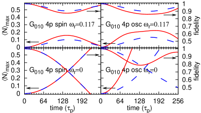
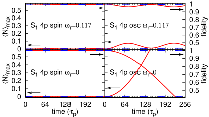
When the sequence 4p is applied with 1st-order self-refocusing pulses (Hermitian or $S_{L}$), the first-order terms in the effective Hamiltonian are gone. This leaves terms linear in $\tau_{p}$ as the leading-order correction

$$H_{\bf 4p} = \omega_{r}b^{\dagger}b-i{\tau_{p}g\omega_{r}\over 4}\sigma_{x}(b^{\dagger}-b)\hskip 93.95122pt$$ (38)

$$-i{1+4\zeta\over 8}\tau_{p}g^{2}\sigma_{z}(b^{2}-\mathrm{h.c.})+\mathcal{O}(s,\alpha\tau_{p},\tau_{p}^{2})$$

where we set $s=0$ and dropped the relatively small term $\propto\alpha\tau_{p}$. We note that the first two terms in Eq. (38) disappear with $\omega_{r}=0$. The third term is suppressed when the oscillator is replaced by an auxiliary qubit ($b\to\tau_{-}$, $b^{\dagger}\to\tau_{+}$, $b^{\dagger}b\to\tau_{z}/2$). The same happens if the sequence is applied in the $x$-$z$ direction [sequence $\mathbf{4p}(xz)=X\overline{Z}XZ$], with the corresponding effective Hamiltonian

$$H_{\bf 4p}^{(xz)} = \omega_{r}b^{\dagger}b+{isg\over 4}\sigma_{x}(b^{\dagger}-b)$$ (39)

$$+i{\tau_{p}g\omega_{r}\over 4}\sigma_{x}(b^{\dagger}-b)+\mathcal{O}(s\tau_{p},\alpha\tau_{p},\tau_{p}^{2}).$$

The net effect is that the refocusing accuracy is dramatically improved when the oscillator is replaced by an auxiliary qubit, or when the four-pulse sequence is applied in the $x$-$z$ plane, with the additional mode being in resonance with the qubit. In such cases, the only remaining linear in $\tau_{p}$ terms in the effective Hamiltonian are those proportionaly to the small parameter $\alpha$, and the refocusing gets much more accurate, see Fig. 2.

V.2 Sequence 8a

The antisymmetric eight-pulse sequence 8a produces the effective Hamiltonian

$$H_{\mathbf{8a}}=\omega_{r}b^{\dagger}b+{isg\over 4}\sigma_{z}(b^{\dagger}-b)+\mathcal{O}(\tau_{p}^{2}).$$ (40)

The refocusing is 1st-order with Gaussian pulses (Fig. 3), with the errors comparable to those of the sequence 4p (cf. Fig. 1). With self-refocusing pulses S₁ [Fig. 4] or Q₁ (not shown) the sequence produces 2nd-order refocusing. With all 1st and 2nd-order error terms cancelled, the refocusing accuracy is improved substantially.

Figure 3: (color online) As in Fig. 1 but for the sequence 8a. The term $\propto s$ in Eq. (40) produces large errors comparable for those for 4p sequence in Fig. 1. This indicates that this sequence is less stable to pulse shape errors as, e.g., the symmetric sequence 8s.

Figure 4: (color online) As in Fig. 1 but for the sequence 8a with pulses S₁. The corresponding curves for pulses Q₁ (not shown) are virtually identical with linear scale.

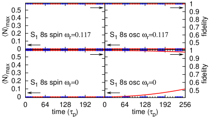
V.3 Sequence 8s

The symmetric eight-pulse sequence 8s produces the effective Hamiltonian

$$H_{\mathbf{8s}}=\omega_{r}b^{\dagger}b-{\alpha g^{2}\tau_{p}\over 8}\sigma_{y}(b^{\dagger}+b)^{2}+\mathcal{O}(s\tau_{p},\tau_{p}^{2})$$ (41)

which corresponds to Eq. (38) with the larger terms already suppressed. The refocusing is first-order with either Gaussian [Fig. 5] or 1st-order pulses [see Fig. 6 with pulses S₁], and second-order with second-order pulses $Q_{L}$ (not shown). With the linear scale of our plots, there is only a slight difference between zeroth and first order pulses (due to higher-order terms), and no visible difference between pulses S₁ and Q₁.

We note that the performance of this sequence is very close to that of the antisymmetric sequence 8a. Nevertheless, the symmetric sequence 8s provides better stability with respect to the pulse shape errors, and it is also expected to result in better visibility (initial decoherence in Ref. Pryadko and Sengupta (2006)) when used in an open system.

Figure 5: (color online) As in Fig. 1 but for the sequence 8s.

Figure 6: (color online) As in Fig. 1 but for the sequence 8s with pulses S₁. Formally, the sequence is of the same order as with Gaussian pulses, see Fig. 5; the noticeable differences are due to error terms of higher order which we dropped in our calculations. The off-resonance refocusing is excellent (the fidelity and $\langle N\rangle$ curves in the top right panel run along the corresponding axes), while the on-resonance performance is also good. The plots with second-order pulses Q₁ (not shown) look almost identical. Note also that with the linear scale of these plots, the curves here are almost indistinguishable from those in Fig. 4.

V.4 Discussion

Our simulations show that with properly designed refocusing, to an excellent accuracy, the quantum oscillator coupled to the qubit remains in the ground state, while the qubit fidelity remains very close to unity. Numerical results agree with the predictions from the analytically computed effective Hamiltonians which show greately reduced coupling between the qubit and the oscillator. Then, in the closed system, a very small frequency bias (of order of renormalized coupling value) becomes sufficient to effectively disconnect the oscillator mode and protect the qubit coherence. Similar effect can be achieved when the finite width $\Gamma$ of the resonance is taken into account: for refocusing to be effective, $\Gamma$ must be large compared with the renormalized qubit coupling.

In other words, refocusing is effective as long as the renormalized qubit coupling with the resonant mode is small on the scale of the resonance width. This gives the modified, more broadely applicable, criterion for applicability of the results of Ref. Pryadko and Sengupta (2006). In particular, we expect the second-order sequence 8s with 2nd-order pulses Q_n to provide an excellent refocusing accuracy to system Hamiltonian of Jaynes-Cummings form (36) also in the presence of a thermal bath, as long as the refocusing rate is sufficiently high. In addition to the condition on renormalized value of the high-$Q$ oscillator mode coupling, the refocusing period $\tau$ must be below the threshold value of order of the inverse bath cut-off frequency refocusing frequency, $\omega_{c}^{-1}$, see Ref. Pryadko and Sengupta, 2006.

VI Conclusions.

In this work we analyzed the performance of soft-pulse dynamical decoupling in the presence of a sharp resonance mode. Because of the associated memory effects, such a problem cannot be addressed by considering master-equation dynamics for the qubit-system density matrix alone. Instead, we included the resonant mode and the corresponding couplings in the system Hamiltonian, and considered the dynamics of the resulting closed quantum system driven by a sequence of soft or hard refocusing pulses applied to the qubit. The analysis was done in terms of the effective Hamiltonian theory which describes the evolution of the system “stroboscobically” at the time moments commensurate with the refocusing period.

In fact, to make our results applicable to a large number of possible coupling terms between the qubit and the oscillator, we solved a more general problem of an arbitrary coupled [see Eq. (14)] controlled qubit. The main result of this work is the expansion of the unitary evolution operator (19), (25) and the classification of the corresponding parameters in Tab. 1. This allows an explicit computation of the error operators associated with refocusing in systems of arbitrary complexity.

We also computed the effective Hamiltonians for several single-qubit refocusing sequences. To quadratic order, all coupling terms are cancelled if the length-8 sequences 8a [Eq. (35)] or 8s [Eq. (34)] are used with 1st or 2nd-order self-refocusing pulses respectively. We illustrated the general analytical results on the specific example of the driven Jaynes-Cummings Hamiltonian. The results of simulations agree with the predictions based on the analytically computed second-order effective Hamiltonians, although in some cases the effects of higher-order terms not included in the calculation are noticeable.

For robust single-qubit refocusing, we recommend the symmetric 8-pulse sequence 8s applied with second-order self-refocusing pulses. This sequence provides excellent refocusing accuracy for any form of the coupling of the qubit with outside world, and it is stable with respect to pulse shape errors. As the second-order symmetric sequence, it should also work well for open systems, as long as the environment is slow on the scale of the refocusing ratePryadko and Sengupta (2006). The thermal bath is expected to remain close to equilibrium, and refocusing to perform well, as long as sharp features in the spectral function are wide on the scale of the renormalized value of the corresponding couplings.

VII Acknowledgements.

This research was supported in part by the NSF grant No. 0622242 (LP) and the Dean’s Undergraduate Research fellowship at UCR (GQ).

References

- Slichter (1992) C. P. Slichter, Principles of Magnetic Resonance (Springer-Verlag, New York, 1992), 3rd ed.
- Freeman (1998) R. Freeman, Progr. NMR Spectr. 32, 59 (1998).
- Vandersypen and Chuang (2004) L. M. K. Vandersypen and I. L. Chuang, Reviews of Modern Physics 76, 1037 (2004).
- Waugh et al. (1968a) J. S. Waugh, L. M. Huber, and U. Haeberlen, Phys. Rev. Lett. 20, 180 (1968a).
- Waugh et al. (1968b) J. S. Waugh, C. H. Wang, L. M. Huber, and R. L. Vold, J. Chem. Phys. 48, 652 (1968b).
- Kofman and Kurizki (2001) A. G. Kofman and G. Kurizki, Phys. Rev. Lett. 87, 270405 (2001).
- Kofman and Kurizki (2004) A. G. Kofman and G. Kurizki, Phys. Rev. Lett. 93, 130406 (2004).
- Pryadko and Sengupta (2006) L. P. Pryadko and P. Sengupta, Phys. Rev. B 73, 085321 (2006).
- Villas-Boas et al. (2004) J. M. Villas-Boas, S. E. Ulloa, and N. Studart, Phys. Rev. B 70, 041302 (2004).
- Cirac and Zoller (1995) J. Cirac and P. Zoller, Phys. Rev. Lett. 74, 4091 (1995).
- Vitali and Tombesi (1999) D. Vitali and P. Tombesi, Phys. Rev. A 59, 4178 (1999).
- You (2001) L. You, Phys. Rev. A 64, 012302 (2001).
- Kielpinski et al. (2002) D. Kielpinski, C. Monroe, and D. J. Wineland, Nature 417, 709 (2002).
- Vitali and Tombesi (2002) D. Vitali and P. Tombesi, Phys. Rev. A 65, 012305 (2002).
- Platzman and Dykman (1999) P. M. Platzman and M. I. Dykman, Science 284, 1967 (1999).
- Dykman and Platzman (2000) M. I. Dykman and P. M. Platzman, Fortschr. Phys. 48, 1095 (2000).
- Lea et al. (2000) M. J. Lea, P. G. Frayne, and Y. Mukharsky, Fortschr. Phys. 48, 1109 (2000).
- (18) M. I. Dykman, P. M. Platzman, and P. Seddighrad, Phys. Rev. B 67, 155402 (2003).
- Pritchett and Geller (2005) E. J. Pritchett and M. R. Geller, Phys. Rev. A 72, 010301 (2005).
- Kapale et al. (2005) K. T. Kapale, G. S. Agarwal, and M. O. Scully, Phys. Rev. A 72, 052304 (2005).
- Wei et al. (2005) L. F. Wei, Y. Xi Liu, and F. Nori, Phys. Rev. B 71, 134506 (2005).
- Geller and Cleland (2005) M. R. Geller and A. N. Cleland, Phys. Rev. A 71, 032311 (2005).
- Blais et al. (2007) A. Blais, J. Gambetta, A. Wallraff, D. I. Schuster, S. M. Girvin, M. H. Devoret, and R. J. Schoelkopf, Phys. Rev. A 75, 032329 (2007).
- Hahn (1950) E. L. Hahn, Phys. Rev. 80, 580 (1950).
- Khodjasteh and Lidar (2005) K. Khodjasteh and D. A. Lidar, Phys. Rev. Lett. 95, 180501 (2005).
- Khodjasteh and Lidar (2007) K. Khodjasteh and D. A. Lidar, Phys. Rev. A 75, 062310 (2007).
- Domb and Green (1974) C. Domb and M. S. Green, eds., Phase transitions and critical phenomena, vol. 3 (Academic, London, 1974).
- Sengupta and Pryadko (2005) P. Sengupta and L. P. Pryadko, Phys. Rev. Lett. 95, 037202 (2005).
- Viola and Lloyd (1998) L. Viola and S. Lloyd, Phys. Rev. A 58, 2733 (1998).
- Warren (1984) W. S. Warren, J. Chem. Phys. 81, 5437 (1984).
- Geen and Freeman (1991) H. Geen and R. Freeman, J. Mag. Res. 93, 93 (1991).
- Bauer et al. (1984) C. Bauer, R. Freeman, T. Frenkiel, J. Keeler, and A. J. Shaka, J. Mag. Res. 58, 442 (1984).