Autoionization of spin-polarized metastable helium in tight anisotropic harmonic traps

Abstract

Spin-dipole mediated interactions between tightly confined metastable helium atoms couple the spin-polarized quintet ${}^{5}\Sigma^{+}_{g}$ state to the singlet ${}^{1}\Sigma^{+}_{g}$ state from which autoionization is highly probable, resulting in finite lifetimes for the trap eigenstates. We extend our earlier study on spherically symmetric harmonic traps to the interesting cases of axially symmetric anisotropic harmonic traps and report results for the lowest 10 states in ”cigar-like” and ”pancake-like” traps with average frequencies of 100 kHz and 1 MHz. We find that there is a significant suppression of ionization, and subsequent increase in lifetimes, at trap aspect ratios $A=p/q$, where $p$ and $q$ are integers, for those states that are degenerate in the absence of collisions or spin-dipole interactions.

I Introduction

There is significant interest in the study and control of quantum processes involving tightly trapped ultracold neutral atoms where the trapping environment modifies the collision properties of the atoms Nature ; Bolda ; Peach04 . Optical lattices, with typical trapping frequencies of $10^{4}$ to $10^{6}$ Hz, have recently been used to study quantum phase transitions and other phenomena in alkali systems Stock and there are now proposals to trap metastable helium and neon in optical lattices Koel04 ; Moal06 ; Vassen06 . Trapped metastable rare gas atoms offer exciting experimental detection strategies to study quantum gases as the large internal energy can be released through Penning and associative ionization during interatomic collisions and through ejection of electrons when the atoms strike a metal surface. The metastable atoms are generally spin-polarized in order to suppress the autoionization rate and to thereby attain large numbers of trapped atoms.

Spin-dipole interactions between the confined metastable helium atoms couple the spin-polarized quintet ${}^{5}\Sigma^{+}_{g}$ state to the singlet ${}^{1}\Sigma^{+}_{g}$ state from which Penning and associative ionization are highly probable. This spin-dipole induced coupling results in finite lifetimes for the trap eigenstates and has been studied for spherically symmetric harmonic traps by Beams04 using a second-order perturbative treatment of the interaction.

In this paper we extend these calculations to the interesting case of anisotropic harmonic traps where there arises the possibility of enhancement and/or suppression of the ionization losses due to interference between the anisotropic part of the trap potential and the spin-dipole interaction which are both proportional to a second order spherical harmonic $Y_{2m}(\theta,\phi)$. In particular we consider traps with axial symmetry about the $z$ axis. These traps have $m=0$ and an asymmetry parameter $\beta$ which ranges from $\beta=2$ for a ”pancake” trap to $\beta=-1$ for a ”cigar” trap.

We have calculated the lowest 10 eigenstates of $\bar{\omega}/2\pi=100$ kHz and 1.0 MHz traps where $\bar{\omega}$ is the mean angular frequency of the trap. We find evidence that the ionization is strongly suppressed and the lifetimes of the trap states significantly lengthened for particular values of $\beta$, especially for the higher states considered.

II Two-atom collisions in an anisotropic harmonic trap

II.1 Hamiltonian

Consider two trapped atoms with masses $M_{1}$ and $M_{2}$, position vectors $\bm{r}_{1}$ and $\bm{r}_{2}$, and electronic spin operators $\bm{S}_{1}$ and $\bm{S}_{2}$ subject to a central interatomic potential $V^{\text{el}}(r)$, where $r=|\bm{r}|=|\bm{r}_{1}-\bm{r}_{2}|$, and a spin-dipole interaction Beams04

$$H_{\text{sd}}(\bm{r})=-\frac{k}{\hbar^{2}r^{3}}\left[3(\bm{S}_{1}\cdot\hat{\bm{r}})(\bm{S}_{2}\cdot\hat{\bm{r}})-\bm{S}_{1}\cdot\bm{S}_{2}\right].$$ (1)

Here $\hat{\bm{r}}=\bm{r}/r$ is a unit vector directed along the internuclear axis and

$$k=\alpha^{2}\left(\frac{\mu_{e}}{\mu_{B}}\right)^{2}E_{h}a_{0}^{3},$$ (2)

where $\alpha$ is the fine structure constant, $a_{0}$ is the Bohr radius, $(\mu_{e}/\mu_{B})$ is the electron magnetic moment to Bohr magneton ratio and $E_{h}=\alpha^{2}m_{e}c^{2}$ is the Hartree energy. Provided the trapping potential is harmonic, the two-atom Hamiltonian is separable into center-of-mass and relative motions. The Hamiltonian for the relative motion is then

$$H=-\frac{\hbar^{2}}{2M}\;\nabla^{2}_{r}+V^{\text{el}}(r)+H_{\text{sd}}(\bm{r})+V_{\text{trap}}(\bm{r})$$ (3)

where $M=M_{1}M_{2}/(M_{1}+M_{2})$ is the reduced mass of the system.

The potential for a general anisotropic harmonic trap

$$V_{\text{trap}}(\bm{r})=\frac{M}{2}\;\left(\omega_{x}^{2}x^{2}+\omega_{y}^{2}y^{2}+\omega_{z}^{2}z^{2}\right),$$ (4)

where $\omega_{x},\omega_{y}$ and $\omega_{z}$ are the trapping frequencies in the $x$, $y$ and $z$ directions, can be resolved into isotropic and anisotropic components by introducing the spherical basis $x_{\mu},\mu=0,\pm 1,$ where

$$x_{\pm}=\mp\frac{1}{\sqrt{2}}(x\pm iy),\quad x_{0}=z.$$ (5)

Noting that $x_{\mu}=rC^{1}_{\mu}(\theta,\phi)$ where

$$C^{l}_{m}(\theta,\phi)\equiv\sqrt{\frac{4\pi}{2l+1}}\;Y_{lm}(\theta,\phi)$$ (6)

is the modified spherical harmonic then, using the product formula

$$C^{1}_{m_{1}}(\theta,\phi)C^{1}_{m_{2}}(\theta,\phi) = \frac{(-1)^{m_{1}}}{3}\;\delta_{m_{1},-m_{2}}\;C^{0}_{0}(\theta,\phi)$$ (7)

$$+\sqrt{\frac{2}{3}}C(1,1,2;m_{1},m_{2},m_{1}+m_{2})$$

$$\times C^{2}_{m_{1}+m_{2}}(\theta,\phi)$$

where $C(j_{1},j_{2},j;m_{1},m_{2},m)$ is the Clebsch-Gordan coefficient, $V_{\text{trap}}(\bm{r})$ can be written as

$$V_{\text{trap}}(\bm{r})=V_{\text{trap}}^{\text{iso}}(r)+V_{\text{trap}}^{\text{aniso}}(r,\theta,\phi).$$ (8)

The isotropic component is

$$V_{\text{trap}}^{\text{iso}}(r)=\frac{M}{2}\bar{\omega}^{2}r^{2}$$ (9)

and the anisotropic part is

$$V_{\text{trap}}^{\text{aniso}}(r,\theta,\phi) = V_{\text{trap}}^{\text{iso}}(r)\;\left\{\frac{\alpha}{\sqrt{6}}\left[C^{2}_{2}(\theta,\phi)+C^{2}_{-2}(\theta,\phi)\right]\right.$$ (10)

$$\left.+\beta\;C^{2}_{0}(\theta,\phi)\right\}.$$

We have introduced the mean square frequency

$$\bar{\omega}^{2}\equiv\frac{1}{3}(\omega_{x}^{2}+\omega_{y}^{2}+\omega_{z}^{2})$$ (11)

and the anisotropy parameters

$$\alpha\equiv\frac{\omega_{x}^{2}-\omega_{y}^{2}}{\bar{\omega}^{2}},\quad\beta\equiv\frac{1}{3\bar{\omega}^{2}}(2\omega_{z}^{2}-\omega_{x}^{2}-\omega_{y}^{2}).$$ (12)

For axially symmetric traps $\omega_{x}=\omega_{y}$ and $\alpha=0$. The parameter $\beta$ then varies over the range $-1\leq\beta\leq 2$ where $\beta=-1$ corresponds to an infinitely long cigar-shaped trap and $\beta=2$ to an infinitesimally thin pancake-shaped trap.

II.2 Perturbation theory

The spin-dipole interaction is of $O(\alpha^{2})$ and can be treated as a perturbation. The unperturbed Hamiltonian $H_{0}$ is then that for ultracold collisions in an anisotropic harmonic trap. The two colliding atoms with spin quantum numbers $S_{1}$ and $S_{2}$ are in the total spin state $|(S_{1}S_{2})SM_{S}\rangle$ where $M_{S}$ is the projection of $S$ onto the space-fixed $z$ axis. During the collision they form the molecular state ${}^{2S+1}\Lambda$ where $\Lambda$ is the projection of the total electronic orbital angular momentum along the molecular axis. The adiabatic potential of this state will be denoted by $V^{\text{el}}_{\Lambda S}(r)$. The appropriate channel states are Beams06

$$|\Phi_{a}\rangle=|\Gamma SM_{S}\rangle|lm\rangle$$ (13)

where $a=\{\Gamma,S,M_{S},l,m\}$ and $|lm\rangle=Y_{lm}(\theta,\phi)$ are the relative motion states. The label $\Gamma$ represents the remaining quantum numbers $S_{1},S_{2},\ldots$ needed to fully specify the channel. The unperturbed Hamiltonian $H_{0}$ is given by

$$H_{0}=-\frac{\hbar^{2}}{2M}\nabla^{2}_{r}+V^{\text{el}}_{\Lambda S}(r)+V_{\text{trap}}(\bm{r})\equiv H^{\text{iso}}_{0}+V^{\text{aniso}}_{\text{trap}}(\bm{r})$$ (14)

and the eigenstates $|\Psi_{n}\rangle$ satisfy

$$H_{0}|\Psi_{n}\rangle=E_{n}|\Psi_{n}\rangle\,.$$ (15)

The states $|\Psi_{n}\rangle$ can be expanded in terms of the channel basis defined in (13) so that

$$|\Psi_{n}\rangle=\sum_{a}\;R_{na}(r)|\Phi_{a}\rangle$$ (16)

and we obtain the matrix eigenvalue equation

$$\sum_{a}H_{a^{\prime}a}R_{na}(r)=E_{n}R_{na^{\prime}}(r)$$ (17)

where, assuming the $r$-dependence of the channel states is negligible,

$$H_{a^{\prime}a} = \langle\tilde{\Phi}_{a^{\prime}}|H_{0}|\Phi_{a}\rangle$$ (18)

$$= h^{\text{iso}}_{a^{\prime}}\delta_{a^{\prime},a}+\langle\tilde{\Phi}_{a^{\prime}}|V^{\text{aniso}}_{\text{trap}}|\Phi_{a}\rangle$$

and

$$h^{\text{iso}}_{a} \equiv \langle\tilde{\Phi}_{a}|H^{\text{iso}}_{0}|\Phi_{a}\rangle$$ (19)

$$= -\frac{\hbar^{2}}{2M}\frac{d^{2}}{dr^{2}}+\frac{l(l+1)\hbar^{2}}{2Mr^{2}}+V^{\text{el}}_{\Lambda S}(r)$$

$$+\frac{M\bar{\omega}^{2}}{2}r^{2}.$$

We have distinguished between right eigenvectors $|\Phi_{a}\rangle$ and left eigenvectors $\langle\tilde{\Phi}_{a}|$, see RL , as $H_{0}$ is non-Hermitian for the singlet state. In the absence of the anisotropy term equation (17) decouples to

$$\left[-\frac{\hbar^{2}}{2M}\frac{d^{2}}{dr^{2}}+\frac{l(l+1)\hbar^{2}}{2Mr^{2}}+V^{\text{el}}_{\Lambda S}(r)+\frac{M\bar{\omega}^{2}}{2}r^{2}\right]R_{a}(r)$$

$$=E_{a}R_{a}(r)\,,$$ (20)

where $E_{a}=2\hbar\bar{\omega}(n^{*}_{r}+l/2+3/4)$ are the energy eigenvalues, see Peach04 , of an isotropic harmonic trap of frequency $\bar{\omega}$. The quantum number $n^{*}_{r}=n_{r}-\mu$ replaces the usual integer $n_{r}\geq 0$ labelling the eigenenergies of a three-dimensional isotropic oscillator and includes the effect of collisions through the quantum defect $\mu$ which depends on $\{\Lambda,S,l\}$.

The channel basis elements in (17) can be evaluated using standard techniques. From (10) we have

$$\langle\tilde{\Phi}_{a^{\prime}}|V^{\text{aniso}}_{\text{trap}}|\Phi_{a}\rangle=\delta_{\gamma^{\prime},\gamma}\langle l^{\prime}m^{\prime}|V^{\text{aniso}}_{\text{trap}}|lm\rangle$$ (21)

where $\gamma=\{\Gamma,S,M_{S}\}$. Using the Wigner-Eckart theorem then gives

$$\langle\tilde{\Phi}_{a^{\prime}}|V^{\text{aniso}}_{\text{trap}}|\Phi_{a}\rangle=V^{\text{iso}}_{\text{trap}}(r)D^{\text{trap}}_{a^{\prime}a}$$ (22)

where

$$D^{\text{trap}}_{a^{\prime}a} = \left\{\alpha\left[C(l,2,l^{\prime};m,2,m^{\prime})+C(l,2,l^{\prime};m,-2,m^{\prime})\right]\right.$$ (23)

$$\left.+\beta C(l,2,l^{\prime};m,0,m^{\prime})\right\}\langle l^{\prime}||\bm{C}^{2}||l\rangle\delta_{\gamma^{\prime},\gamma}.$$

The reduced matrix element is given by

$$\langle l^{\prime}||\bm{C}^{2}||l\rangle=\left[\frac{2l+1}{2l^{\prime}+1}\right]^{\frac{1}{2}}\;C(l,2,l^{\prime};0,0,0).$$ (24)

To second order, the change in energy of the state $|\Psi_{n}\rangle$ due to the perturbation $H_{\text{sd}}$ is

$$\Delta E_{n}=\Delta E^{(1)}_{n}+\Delta E^{(2)}_{n},$$ (25)

where

$$\Delta E^{(1)}_{n}=\langle\tilde{\Psi}_{n}|H_{\text{sd}}|\Psi_{n}\rangle$$ (26)

and

$$\Delta E^{(2)}_{n}=\sum_{m\neq n}\;\frac{\langle\tilde{\Psi}_{n}|H^{\dagger}_{\text{sd}}|\Psi_{m}\rangle\langle\tilde{\Psi}_{m}|H_{\text{sd}}|\Psi_{n}\rangle}{E_{n}-E_{m}}.$$ (27)

The evaluation of the first order correction is straightforward. The second order correction is conveniently evaluated by introducing Pert2 the operator $\hat{F_{n}}$ which satisfies

$$\langle\tilde{\Psi}_{m}|[\hat{F}_{n},H_{0}]|\Psi_{n}\rangle = \langle\tilde{\Psi}_{m}|H_{\text{sd}}|\Psi_{n}\rangle$$ (28)

$$= (E_{n}-E_{m})\langle\tilde{\Psi}_{m}|\hat{F}_{n}|\Psi_{n}\rangle$$ (29)

for $m\neq n$. Invoking the closure relation $\sum_{m}|\Psi_{m}\rangle\langle\tilde{\Psi}_{m}|=I$ then gives

$$\Delta E^{(2)}_{n}=\langle\tilde{\Psi}_{n}|H_{\text{sd}}\hat{F}_{n}|\Psi_{n}\rangle-\langle\tilde{\Psi}_{n}|H_{\text{sd}}|\Psi_{n}\rangle\langle\tilde{\Psi}_{n}|\hat{F}_{n}|\Psi_{n}\rangle.$$ (30)

Equation (28) yields the inhomogeneous equation

$$[\hat{F}_{n},H_{0}]|\Psi_{n}\rangle=(H_{\text{sd}}-\Delta E^{(1)}_{n})|\Psi_{n}\rangle$$ (31)

so that, expanding $\hat{F}_{n}|\Psi_{n}\rangle$ in the channel basis (13)

$$\hat{F}_{n}|\Psi_{n}\rangle=\sum_{a}\;f_{na}(r)|\Phi_{a}\rangle$$ (32)

gives the coupled equations

$$\sum_{a}[E_{n}\delta_{a^{\prime},a}-H_{a^{\prime}a}]f_{na}(r)=\sum_{a}[\langle\tilde{\Phi}_{a^{\prime}}|H_{\text{sd}}|\Phi_{a}\rangle$$

$$-\Delta E^{(1)}_{n}\delta_{a^{\prime},a}]R_{na}(r).$$ (33)

To evaluate the elements for the spin-dipole interaction we note that the interaction may be written as the scalar product of two second-rank irreducible tensors, see Beams04 ,

$$H_{\text{sd}}=V_{\text{sd}}(r)\bm{T}^{2}\bm{\cdot}\bm{C}^{2},$$ (34)

where $\bm{T}^{2}$ is

$$T^{2}_{\nu}\equiv\left[\bm{S}^{1}_{1}\bm{\times}\bm{S}^{1}_{2}\right]^{2}_{\nu}=\sum_{\mu}C(1,1,2;\mu,\nu-\mu,\nu)\;S^{1}_{1,\mu}S^{1}_{2,\nu-\mu},$$ (35)

and $\bm{C}^{2}$ is the second rank tensor formed from the modified spherical harmonics. The radial factor is $V_{\text{sd}}(r)=b/r^{3}$ where $b\equiv-\sqrt{6}k/\hbar^{2}$. We then get

$$\langle\Phi_{a^{\prime}}|H_{\text{sd}}|\Phi_{a}\rangle=V_{\text{sd}}(r)D^{\text{sd}}_{a^{\prime}a}$$ (36)

where, by invoking the Wigner-Eckart theorem, we find Beams06

$$D^{\text{sd}}_{a^{\prime}a} = \delta_{M_{S^{\prime}}+m^{\prime},M_{S}+m}\;(-1)^{M_{S^{\prime}}-M_{S}}$$ (37)

$$\times C(S,2,S^{\prime};M_{S},M_{S^{\prime}}-M_{S},M_{S^{\prime}})$$

$$\times C(l,2,l^{\prime};m,m^{\prime}-m,m^{\prime})$$

$$\times\langle\Gamma^{\prime}S^{\prime}||\bm{T}^{2}||\Gamma S\rangle\langle l^{\prime}||\bm{C}^{2}||l\rangle.$$

The reduced matrix element of $\bm{T}^{2}$ is given by

$$\langle\Gamma^{\prime}S^{\prime}||\bm{T}^{2}||\Gamma S\rangle = \delta_{\Gamma^{\prime},\Gamma}\;\delta_{S_{1}^{\prime},S_{1}}\;\delta_{S_{2}^{\prime}S_{2}}\;\hbar^{2}$$ (41)

$$\times\sqrt{S_{1}(S_{1}+1)S_{2}(S_{2}+1)}$$

$$\times\left[\begin{array}[]{lll}S_{1}&S_{2}&S\\ 1&1&2\\ S_{1}&S_{2}&S^{\prime}\end{array}\right],$$

where the angular momentum coefficient in (41) is related to the Wigner $9-j$ coefficient

$$\left[\begin{array}[]{lll}j_{1}&j_{2}&j\\ k_{1}&k_{2}&k\\ j_{1}^{\prime}&j_{2}^{\prime}&j^{\prime}\end{array}\right] \equiv [(2j_{1}^{\prime}+1)(2j_{2}^{\prime}+1)(2j+1)(2k+1)]^{\frac{1}{2}}$$ (49)

$$\times\left\{\begin{array}[]{lll}j_{1}&j_{2}&j\\ k_{1}&k_{2}&k\\ j_{1}^{\prime}&j_{2}^{\prime}&j^{\prime}\end{array}\right\}.$$

In terms of the channel basis expansions, the energy shifts are given by

$$\Delta E^{(1)}_{n}=\sum_{a^{\prime},a}\;D^{\text{sd}}_{a^{\prime}a}\langle\tilde{R}_{na^{\prime}}|V_{\text{sd}}|R_{na}\rangle$$ (50)

and

$$\Delta E^{(2)}_{n}=\sum_{a^{\prime},a}\;D^{\text{sd}}_{a^{\prime}a}\langle\tilde{R}_{na^{\prime}}|V_{\text{sd}}|f_{na}\rangle-\Delta E^{(1)}_{n}\sum_{a}\langle\tilde{R}_{na}|f_{na}\rangle.$$ (51)

III Application to ultracold spin-polarized metastable helium atoms

We now consider application of the theory to spin-polarized metastable helium atoms tightly confined in axially symmetric harmonic traps for which the asymmetry parameter $\alpha$ in (12) vanishes. The colliding atoms are in the $|(S_{1}S_{2})SM_{S}\rangle=|(11)22\rangle$ ${}^{5}\Sigma_{g}^{+}$ molecular state but, noting that the reduced matrix elements for the spin-dipole interaction are Beams06 $\langle\Gamma^{\prime}2||\bm{T}^{2}||\Gamma 2\rangle=\delta_{\Gamma^{\prime},\Gamma}\;\hbar^{2}\sqrt{{7}/{3}}$ and $\langle\Gamma^{\prime}0||\bm{T}^{2}||\Gamma 2\rangle=-\delta_{\Gamma^{\prime},\Gamma}\;\hbar^{2}\sqrt{{5}/{3}}$ ($\langle\Gamma^{\prime}1||\bm{T}^{2}||\Gamma 2\rangle$ vanishes by symmetry of the $9-j$ symbol), then the spin-dipole interaction couples this state to the $|(11)00\rangle$ ${}^{1}\Sigma^{+}_{g}$ state from which Penning and associative ionization processes are highly probable. We model these ionization processes from the singlet state using a complex optical potential of the form $V(r)-i\Gamma(r)/2$ where $\Gamma(r)$ is the ionization width. This coupling between the initial quintet state and the singlet state produces complex energy shifts $\Delta E_{n}=\Delta E_{n}^{\text{re}}-i\gamma_{n}/2$ due to the complex form of the singlet potential. The $1/e$ lifetimes of the trap states will be $\tau_{n}=\hbar/\gamma_{n}$ .

The eigenvalue equations (17) for $R_{na}(r)$ and the coupled differential equations (II.2) for the perturbed functions $f_{na}(r)$ were solved using a discrete variable representation and a scaled radial coordinate grid $\rho=r/\xi=\zeta t^{\sigma}$ where $\xi=\sqrt{\hbar/M\bar{\omega}}$ is the effective range of the oscillator ground state and $\zeta$ and $\sigma$ are scaling parameters (see Peach04 for details). We note that the bosonic symmetry of the identical metastable helium atoms restricts the scattering to even partial waves in the expansions (16) and (32).

As input to the problem we require the Born-Oppenheimer potentials for both the ${}^{5}\Sigma_{g}^{+}$ and ${}^{1}\Sigma_{g}^{+}$ electronic states of the metastable helium dimer. For the ${}^{5}\Sigma_{g}^{+}$ potential we have used the full potential $V^{5}_{\text{PJ}}(r)$ of Przybytek and Jeziorski Przyb05 which includes adiabatic and relativistic corrections, adjusted to match the experimental binding energy of the least bound ($v=14$) state Moal06 . For the singlet potential we use a potential $V^{1}_{\text{M}}$ constructed from the short-range potential of Müller et al Muller91 exponentially damped onto the quintet potential at long range Venturi99 . Also required is the ionization width $\Gamma(r)$. Two forms were used, $\Gamma_{\text{M}}(r)$ obtained from a least squares fit to the tabulated results in Muller91 and the simpler form $\Gamma_{\text{GMS}}(r)=0.3\exp(-r/1.086)$ advocated in Garrison73 .

IV Results and Discussion

We have calculated the lifetimes of the lowest 10 trap states for axially symmetric anisotropic harmonic traps with average trapping frequencies of 100 kHz and 1 MHz. We label these states $v=0,\ldots,9$.

With the power law scaling $\sigma=10$, three to four digit convergence with respect to the radial grid was obtained using 500 (450) grid points for $\bar{\omega}/2\pi=100$ kHz (1 MHz) and an outer boundary set at $15\xi$. The position of the outer boundary was determined by the requirement that the states up to at least $v=9$ were insensitive to its position. A similar three to four digit convergence with respect to the number of partial waves included was generally obtained with six partial waves ($l=0,2,\ldots,10$) for asymmetry values in the range $-0.9\leq\beta\leq 1.9$, where $\Delta\beta=0.01$. However, for some of the cases where the lifetimes are strongly enhanced (see below), satisfactory partial wave convergence was not obtained and the results reported for these cases should be regarded as indicative only.

The lifetimes of the six lowest states for $\bar{\omega}/2\pi=100$ kHz are shown in Figs 1 and 2 as a function of the trap aspect ratio $A$. For ”cigar-like” traps with $\omega_{x}>\omega_{z}$ the aspect ratio is

$$A=\frac{\omega_{x}}{\omega_{z}}=\sqrt{\frac{(1-\beta/2)}{(1+\beta)}}$$ (52)

whereas for ”pancake-like” traps with $\omega_{z}>\omega_{x}$ it is $A=\omega_{z}/\omega_{x}$.

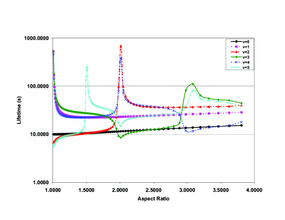
Figure 1: Lifetimes of the six lowest trap states for ”cigar-like” traps with $\bar{\omega}/2\pi=100$ kHz as a function of trap aspect ratio $A=\omega_{x}/\omega_{z}$.

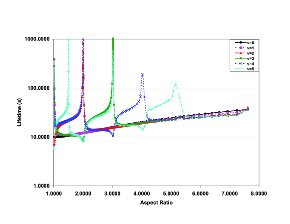
Figure 2: Lifetimes of the six lowest trap states for ”pancake-like” traps with $\bar{\omega}/2\pi=100$ kHz as a function of trap aspect ratio $A=\omega_{z}/\omega_{x}$.

The results display a strong sensitivity of most lifetimes to the aspect ratio $A$, especially around the values $A=p/q$ where $p$ and $q$ are integers. Under higher resolution these peaks show a double peak structure centred on $A=p/q$. In Table 1 results are presented for the 10 lowest states at the $\beta$ values closest to these aspect ratios and it is clear that there is an aspect ratio for nearly every state at which the lifetime is greatly enhanced. The behavior near $A=1$ ($\beta=0$) is also interesting. For $\beta=0$ the states become pure partial waves and those states $v=0,2,5,9$ which contain $l=0$ develop lifetimes which increase slowly for small $|\beta|$ . However the other states show strongly enhanced lifetimes at very small values of $\beta\sim O(10^{-3})$ either side of $\beta=0$. No results are reported for the $v=4,7,8$ states at $A=1$ as for these cases our program developed numerical instabilities due to ill-conditioned matrices at very small $\beta\leq O(10^{-4})$. We note that the results given in Beams04 for the $l=0$ states of a spherically symmetric trap are reproduced for $\beta=0$ if we use the potential $V^{5}_{\text{SM}}(r)$ of Stärck and Meyer Starck94 .

Table 1: Lifetimes (in seconds) of the 10 lowest trap states for axially symmetric anisotropic harmonic traps of selected aspect ratios $A$ and an average trapping frequency of 100 kHz. The upper part of the table is for ”cigar-like” traps where $A=\omega_{x}/\omega_{z}$, the lower part is for ”pancake-like” traps where $A=\omega_{z}/\omega_{x}$. The numbers in parentheses denote powers of 10. For many of the cases of very strongly enhanced lifetimes the results are indicative only as satisfactory partial wave convergence was not achieved.

$A$	$v=0$	$v=1$	$v=2$	$v=3$	$v=4$	$v=5$	$v=6$	$v=7$	$v=8$	$v=9$
1	9.977	5.76(-6)	6.714	1.35(-5)		5.399	2.28(-5)			4.645
1.25	10.14	23.86	9.604	30.55	22.83	9.618	34.19	29.36	22.80	10.04
1.5	10.50	22.44	10.54	27.49	22.42	134.8	8.592	27.44	93.43	17.31
1.75	10.98	22.53	11.91	24.39	23.90	34.66	11.94	26.20	33.67	24.99
2	11.51	23.04	689.5	8.540	384.8	14.78	1.144(3)	941.1	7.135	554.3
2.25	12.01	23.67	40.32	11.38	41.24	22.32	53.39	36.95	11.28	55.80
2.5	12.57	24.46	36.83	12.70	37.42	24.29	47.06	34.21	1.76(3)	10.32
2.75	13.01	25.09	36.50	13.96	33.76	25.80	44.35	33.79	63.40	13.22
3	13.56	25.91	36.76	82.08	11.86	36.17	30.92	36.43	49.55	16.60
3.25	14.02	26.60	37.20	64.36	12.95	54.67	24.51	58.80	31.72	95.24
3.5	14.57	27.44	37.86	52.19	14.49	47.73	26.70	55.57	31.84	73.23
3.75	15.27	28.56	40.11	44.31	18.01	39.35	24.84	59.83	27.37	66.31
1.25	10.16	11.08	18.00	11.24	19.14	25.52	11.14	19.36	26.77	35.07
1.5	10.60	10.95	21.28	10.73	21.73	2.2(2)	8.133	21.34	206.9	8.306
1.75	11.22	11.36	25.85	10.62	26.04	10.90	32.11	25.00	10.44	34.55
2	11.98	11.99	4.0(6)	8.042	6.1(6)	8.017	4.2(3)	3.7(2)	6.451	2.2(2)
2.25	12.80	12.71	14.08	22.30	13.94	21.50	14.89	21.28	29.26	14.34
2.5	13.67	13.50	14.12	27.25	13.67	25.73	14.09	23.91	96.42	10.96
2.75	14.60	14.36	14.71	33.25	13.67	29.99	13.95	28.57	13.88	34.22
3	15.55	15.23	15.41	1.2(2)	11.23	65.20	11.73	39.89	12.46	52.50
3.25	16.57	16.19	16.21	17.98	28.07	17.24	26.14	17.64	22.06	18.29
3.5	17.67	17.19	17.06	17.65	34.87	16.86	30.27	17.24	25.13	17.06
3.75	18.79	18.28	18.21	18.53	43.46	16.95	39.90	16.94	33.72	17.01
4	19.87	19.29	19.12	19.23	1.9(2)	13.82	82.23	14.63	34.53	17.59
4.25	20.82	20.23	20.42	20.95	23.07	36.13	22.20	26.31	20.65	23.55
4.5	21.94	21.22	20.82	20.65	21.71	41.38	20.64	38.00	20.14	31.79
4.75	23.27	22.45	21.88	21.56	22.03	50.10	20.45	43.68	20.16	35.71
5	24.30	23.40	22.68	22.26	22.50	64.85	19.68	51.71	19.62	2.2(3)

To understand this behavior we note that, in the absence of collisions, the energy eigenvalues for an axially symmetric harmonic trap

$$E_{0}^{\text{no-coll}}=\hbar\omega_{x}(n_{x}+\frac{1}{2})+\hbar\omega_{y}(n_{y}+\frac{1}{2})+\hbar\omega_{z}(n_{z}+\frac{1}{2})$$ (53)

can be written as

$$E_{0}^{\text{no-coll}}=\frac{\hbar\bar{\omega}}{2}\sqrt{1+\beta}[2n_{z}+1+2A(n_{x}+n_{y}+1)]$$ (54)

where $A=\omega_{x}/\omega_{z}$. For $A=p/q$ this becomes

$$E_{0}^{\text{no-coll}}=\frac{\hbar\bar{\omega}}{2}\sqrt{\frac{3}{q^{2}+2p^{2}}}[(2n_{z}+1)q+2(n_{x}+n_{y}+1)p].$$ (55)

From (55) it is clear that, for a given pair of integers $(p,q)$, there will be states $(n_{x},n_{y},n_{z})$ that are degenerate. For example, consider the case $(p,q)=(3,2)$ for which the lowest degenerate states $(n_{x},n_{y},n_{z})$ are $(1,1,0),(0,0,3)$, corresponding to the vibrational states $v=(5,6)$ and $(1,1,1),(0,0,4)$ corresponding to $v=(8,9)$. Collisions then break the degeneracies of the eigenstates formed from even partial waves. Inspection of Figs 1 and 2 and Table 1 shows that it is these degenerate oscillator states that have the strongly enhanced lifetimes.

The enhancement of some lifetimes at very small $\beta$ can also be traced to underlying degeneracies. As $\beta\rightarrow 0$, the energies approach the isotropic oscillator eigenvalues

$$E_{0}^{\text{no-coll}}(\beta=0)=\frac{\hbar\bar{\omega}}{2}(4n_{r}+2l+3)$$ (56)

which have the degeneracies $(n_{r},l)=(0,2),(1,0)$ corresponding to $v=1,2$, $(0,4),(1,2),(2,0)$ to $v=3,4,5$ and $(0,6),(1,4),(2,2),(3,0)$ to $v=6,\ldots,9$. Again collisions break some of these degeneracies, predominantly by raising the energies of the $l=0$ states $v=0,2,5,9$.

The results for $\bar{\omega}/2\pi=1$ MHz show the same general features as those for 100 kHz and are not presented here.

In conclusion, our calculations show that the ionization losses are sensitive to the anisotropic trapping environment and that significant suppression of ionization can occur at particular trap aspect ratios. Although there is some dependance of our results on the choice of ionization width $\Gamma(r)$ (the differences in lifetimes obtained using the ionization widths $\Gamma_{\text{M}}$ and $\Gamma_{\text{GMS}}$ are remarkably constant with the $\Gamma_{\text{GMS}}$ results lower by 14.2%) and satisfactory partial wave convergence could not obtained with the limit of six partial waves for some of the strongly enhanced lifetimes, the general features displayed by our results are robust.

References

• (1) For review, see the Special Issue of Nature Insight: Ultracold Matter [Nature (London) 416, 205 (2002)]
• (2) E. L. Bolda, E. Tiesinga, and P. S. Julienne, Phys. Rev. A 66, 013403 (2002); D. Blume and C. H. Greene, Phys. Rev. A 65, 043613 (2002); E. L. Bolda, E. Tiesinga, and P. S. Julienne, Phys. Rev. A 68, 032702 (2003).
• (3) G. Peach, I. B. Whittingham, and T. J. Beams, Phys. Rev. A 70, 032713 (2004).
• (4) See, e.g., R. Stock and I. H. Deutsch, Phys. Rev. A 73, 032701 (2006) and references therein.
• (5) J. C. J. Koelemeij and M. Leduc, Eur. Phys. J. D 31, 263 (2004).
• (6) S. Moal, M. Portier, J. Kim, J. Dugué, U. D. Rapol, M. Leduc, and C. Cohen-Tannoudji, Phys. Rev. Lett. 96, 023203 (2006).
• (7) W. Vassen, T. Jeltes, J. M. McNamara, and A. S. Tychkov, cond-mat/0610414.
• (8) T. J. Beams, G. Peach, and I. B. Whittingham, J. Phys. B: At. Mol. Opt. Phys. 37, 4561 (2004).
• (9) H. Lefebvre-Brion and R. W. Field, The Spectra and Dynamics of Diatomic Molecules (Elsevier, Amsterdam, 2004), Sec. 9.3.1.
• (10) A. Dalgarno and J. T. Lewis, Proc. R. Soc. A 233, 70 (1955); E. Merzbacher, Quantum Mechanics, 3rd ed. (John Wiley and Sons, New York, 1998), Chap. 18.
• (11) T. J. Beams, G. Peach, and I. B. Whittingham, Phys. Rev. A 74, 014702 (2006).
• (12) M. Przybytek and B. Jeziorski, J. Chem. Phys. 123, 134315 (2005).
• (13) M. W. Müller, A. Merz, M.-W. Ruf, H. Hotop, W. Meyer, and M. Movre, Z. Physik D 21, 89 (1991)
• (14) V. Venturi, I. B. Whittingham, P. J. Leo, and G. Peach, Phys. Rev. A 60, 4635 (1999).
• (15) B. J. Garrison, W. H. Miller, and H. F. Schaefer, J. Chem. Phys. 59, 3193 (1973).
• (16) J. Stärck and W. Meyer, Chem. Phys. Lett. 225, 229 (1994).