BFKL at NNLO

Abstract

We present a recent determination of an approximate expression for the $O(\alpha_{s}^{3})$ contribution $\chi_{2}$ to the kernel of the BFKL equation. This includes all collinear and anticollinear singular contributions and is derived using duality relations between the GLAP and BFKL kernels.

1 QCD at small-$x$

Reducing the theoretical uncertainties in cross-sections for hadron colliders requires the computation of higher order contributions in perturbative QCD, both at fixed order and at the resummed level. In particular at high energy colliders such as the LHC, we must be able to control both the logarithms of $Q^{2}$ and $x$ as given by GLAP and BFKL evolution. Fixed–order BFKL kernels, which resum only logs of $x$, have been widely used in many studies (such as saturation and BFKL Monte Carlos for final states). The BFKL kernel has been computed explicitly at the next-to-leading order accuracy [1]; here we present an approximation of the NNLO contribution. The fixed–order expansion of the kernel is known to be slowly convergent, hence the NNLO contribution is important for an accurate assessment of the NLO uncertainty at any particular scale.

Let us consider the GLAP and the BFKL equations:

$$\frac{d}{dt}G(N,t) = \gamma(N,\alpha_{s})G(N,t)\,,$$ (1)

$$\frac{d}{d\xi}G(\xi,M) = \chi(M,\alpha_{s})G(\xi,M)\,,$$ (2)

They describe, respectively, the evolution with respect to $t=ln\frac{Q^{2}}{\mu^{2}}$ and $\xi=ln\frac{s}{Q^{2}}=ln\frac{1}{x}$ of the singlet parton density. The complex variables $N$ and $M$ are the Mellin moments with respect to $x$ and $Q^{2}$ respectively: upon taking moments the integro-differential evolution equations become ordinary differential equations. Note that the GLAP evolved parton density $G$ is integrated over the transverse momenta, while the BFKL equation is usually written in terms of the unintegrated quantity $\mathcal{G}$. We shall return to this issue in the next section.

Eq. (2) is written in the fixed coupling approximation; the introduction of the running of the coupling is nontrivial because upon Mellin transform $\alpha_{s}(t)$ becomes a differential operator:

$$\alpha_{s}(t)=\frac{\alpha_{s}}{1+\alpha_{s}\beta_{0}t} \Longrightarrow \hat{\alpha}_{s}=\frac{\alpha_{s}}{1-\alpha_{s}\beta_{0}\frac{\partial}{\partial M}}\,.$$

As a consequence the BFKL kernel $\chi(\hat{\alpha}_{s},M)$ becomes an operator beyond leading order. It is useful to notice that different arguments for the running coupling correspond to different orderings of the operators.

The fixed-order expansion of the BFKL kernel is:

$$\chi(M,\hat{\alpha}_{s})=\hat{\alpha}_{s}\chi_{0}(M)+\hat{\alpha}^{2}_{s}\chi_{1}(M)+\hat{\alpha}^{3}_{s}\chi_{2}(M)+\dots$$ (3)

It is well known that the NLO order term $\chi_{1}$ is large and has a qualitatively different shape to the leading order kernel $\chi_{0}$. The determination of the NNLO contribution $\chi_{2}$ is motivated not only by the slow convergence of the perturbative expansion but also by the expectation that the NNLO approximation will have the same qualitative shape as the LO thus having better stability proprieties than the NLO. We compute an approximation to the NNLO kernel which includes all the collinear $(M\sim 0)$ and anticollinear $(M\sim 1)$ singularities: this computation is based on so called duality relations between the BFKL kernel and the GLAP anomalous dimension.

2 The collinear approximation of the BFKL
kernel

At fixed coupling, the two evolution equations (1) and (2) admit the same leading twist solution when the kernels are related by:

$$\chi(\gamma(N,\alpha_{s}),\alpha_{s})=N,\qquad\qquad\gamma(\chi(M,\alpha_{s}),\alpha_{s})=M,$$ (4)

and the boundary conditions are suitably matched [2], [3].

The GLAP anomalous dimension $\gamma(N,\alpha_{s})$ has been computed up to NNLO, i.e. $O\left(\alpha_{s}^{3}\right)$ [4]. Using duality it is thus possible to determine the first three coefficients of the Laurent expansion about $M=0$ of the BFKL kernel. This means that we can compute all the collinear singularities of the $O\left(\alpha_{s}^{3}\right)$ contribution: writing

$$\chi_{2}(M)=\frac{c_{2,-3}}{M^{3}}+\frac{c_{2,-2}}{M^{2}}+\frac{c_{2,-1}}{M}+\ldots\,.$$ (5)

the determination of the coefficients $c_{2,-3}$, $c_{2,-2}$ and $c_{2,-1}$ requires the knowledge of the LO, NLO and NNLO anomalous dimension respectively.

At LO the calculation is straightforward because it only involves the inversion of eq. (4), but beyond that several other contributions must be taken into account. More precisely we have to address the following complications:

• The inclusion of running coupling effects.

• The relation between kernels for the integrated and the unintegrated parton density.

• The dependence of the kernel on the factorisation scheme.

• The choice of kinematic variables.

All these issues were well understood at NLO [5], but only recently under control at NNLO.

The frozen coupling hypothesis is no longer valid beyond leading order: duality relations still hold but they receive running coupling contributions [6], [7]. Running coupling duality has been proved to all orders using an operator method. As we already noticed the running coupling in $M$-space is a differential operator; duality states that the BFKL and GLAP solutions coincide if the respective operator kernels are the inverse of each other when acting on physical states. Because of non-vanishing commutation relations the inversions of the kernels is not trivial; the operator formalism enables us to compute the running coupling corrections in an algebraic way, calculating commutators of the relevant operators, e.g.

$$[\hat{\alpha}_{s}^{-1},M]=-\beta_{0}+\alpha_{s}\beta_{0}\beta_{1}+\dots$$ (6)

and express the result in terms of the fixed coupling duals as described extensively in [8].

The BFKL equation describes the evolution of a parton density $\mathcal{G}$ unintegrated over the transverse momenta, while GLAP of the integrated one $G$. The relation between $\mathcal{G}$ and $G$ is given by:

$$\mathcal{G}(N,t)=\frac{d}{dt}G(N,t)\,.$$

This gives the following NNLO relation between unintegrated kernel and the integrated one $\chi^{i}$ derived from duality:

$$\chi_{2}=\chi^{i}_{2}-\beta_{0}\beta_{1}\frac{\chi^{i}_{0}}{M}-2\beta_{0}\frac{\chi^{i}_{1}}{M}\,.$$ (7)

The direct computation of the BFKL kernel is based on determination of the gluon Green’s function in the high energy limit in the framework of the $k_{\perp}$- factorisation theorem. This is compatible with the usual factorisation theorem of collinear singularities but it differs from it by a computable scheme change. This arises from a difference in normalisation between of the gluon Green’s functions which enter the BFKL equation and GLAP equations. The usual computation of the BFKL kernel using gluon Reggeization [1] is performed in the so called $Q_{0}$ scheme [9]. The gluon normalisation factor relating conventional $\overline{MS}$ to the $Q_{0}$ scheme can be factorised as [10]

$$R(N,t)=\mathcal{N}(N,t)\mathcal{R}(N,t)\,,$$ (8)

where $\mathcal{N}$ contains readily calculable running coupling and integrated/unintegrated contributions, while $\mathcal{R}$ is related to the $\overline{MS}$ definition of the anomalous dimension. The leading log-$x$ contribution to the $\mathcal{R}$ scheme change was computed in [11]. We discuss the collinear approximation of the NLL$x$ scheme change in [12], where we show that it can be derived from the analytic continuation of the GLAP anomalous dimension to $d=4-2\varepsilon$ space-time dimensions. However although the $O(\alpha_{s}\varepsilon)$ and $O(\alpha_{s}\varepsilon^{2})$ contributions are known the $O(\alpha_{s}^{2}\varepsilon)$ contribution is not. We assess the uncertainty in our calculation due to this unknown contribution to the scheme change in fig. 2 below.

Once we have all the possible contributions which correct duality relations at NNLO under control, we can compute the collinear approximation of the BFKL kernel in the $Q_{0}$ scheme. In such scheme the result can be extend in the anticollinear region $M\sim 1$ because the kernel is symmetric upon the exchange:

$$M\leftrightarrow 1-M$$ (9)

as a consequence of the symmetry of the diagrams for BFKL processes upon the exchange of the virtualities at the top and the bottom [1], [13]. Before we can exploit this symmetry we must make sure that all sources of symmetry breaking have been removed. The symmetry may be broken by the choice of kinematic variables (e.g. in DIS we choose $x=\frac{Q^{2}}{s}$), and by the argument of the running coupling ($\alpha_{s}(Q^{2})$ in DIS). The BFKL kernel can be written in symmetric variables ($x_{sym}={\sqrt{Q^{2}k^{2}}}/{s}$) thanks to the relation:

$$\chi^{sym}(\hat{\alpha}_{s},M)=\chi^{DIS}(\hat{\alpha}_{s},M+\frac{1}{2}\chi^{sym}(\hat{\alpha}_{s},M))\,.$$ (10)

The kernel in symmetric variables can be extended to the anticollinear region:

$$\chi_{2}^{sym}(\hat{\alpha}_{s},M)=\sum_{j=1,5}c_{2,-j}\left[\hat{\alpha}_{s}^{3}\frac{1}{M^{j}}+\frac{1}{(1-M)^{j}}\hat{\alpha}_{s}^{3}\right]+O(M^{0})\,.$$ (11)

The different order of the operators in the collinear and anticollinear regions corresponds to a symmetric choice for the running coupling. After the symmetrisation one can express the results canonically ordered with all the powers of $\hat{\alpha}_{s}$ on the left. This choice will, of course, break the symmetry of the kernel.

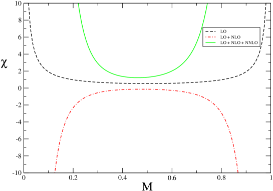
Figure 1: This plot shows the LO, NLO and NNLO approximations to the BFKL kernel in $Q_{0}$-scheme for $\alpha_{s}=0.2$.

The results are plotted in figure $1$. It is clear that the expansion of BFKL kernel is not well behaved (due to the collinear and anticollinear poles at $M=0$ and $M=1$ of increasing order and alternating sign). However, as expected because of the sign of the dominant pole, the BFKL kernel at NNLO has a minimum for every value of the coupling. In figure $2$ we plot the intercept, defined as the value of the kernel in its minimum, as a function of the coupling constant. The inclusion of the NNLO contribution improves the convergence of the perturbative expansion, however for values of the coupling constants relevant for phenomenology (say $\alpha_{s}\gtrsim 0.1$) the series has yet to converge.

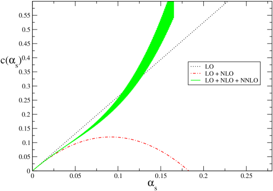
Figure 2: This plot shows the intercept as a function of the coupling, at LO, NLO and NNLO. The error band is due to the unknown term in the scheme change.

3 Discussion

We have seen that thanks to duality relations and the computation of the anomalous dimension at NNLO, the calculation of the collinear approximation of the BFKL kernel at $O(\alpha_{s}^{3})$ can be performed. Here we discuss the accuracy and the limitations of our result.

We have computed an approximation to the forward BFKL kernel, which has been azimuthal averaged over the transverse momenta. The collinear approximation is based on the computation of coefficients of the Laurent series in $M\sim 0$ of the BFKL kernel. Because of the singularities at $M=\pm 1$ this series has radius of convergence one. Similarly the Laurent series for the anticollinear singularities around $M=1$ also has radius of convergence one. Thus we expect the approximate calculations to do well over the central region $0\leq M\leq 1$, but to break down as $M\to-1$, $M\to 2$. In figure $3$ we show how well the approximation actually performs at LO and NLO, where the exact result is known. As expected the agreement is excellent close to $M=0$ and $M=1$, and even in the central region the difference between the collinear approximation and the full result is at the percent level. Hence we can conclude that at leading twist the collinear kernel is a very good approximation to the full LO and NLO ones. For this reason we also expect our result for $\chi_{2}$ to be a good approximation, within a few per cent, for calculations performed at leading twist. A reasonable variation of the unknown contribution to the NLLx scheme change in our calculation changes the kernel $\chi_{2}$ by $\sim 5\%$, hence well within the accuracy we expect for our approximation.

It is well known that beyond NLO BFKL evolution presents various unsolved problems. A direct computation shows that the universality of the pomeron exchange is broken at NNLO [14]. Furthermore a new class of contributions involving the $t$-channel exchange of four gluons enters at NNLO (see [15] and references therein). These are twist-four contributions which can mix with the twist-four part of the two-gluon operators. The form of the full BFKL equation at NNLO is thus different from that at LO and NLO, in contrast to the GLAP equation which has the same form to all orders in perturbation theory. Nevertheless collinear factorisation and running coupling duality guarantee the existence of a universal and factorised leading twist kernel for small-$x$ evolution [8], valid in the approximation where all higher twist contributions are suppressed.

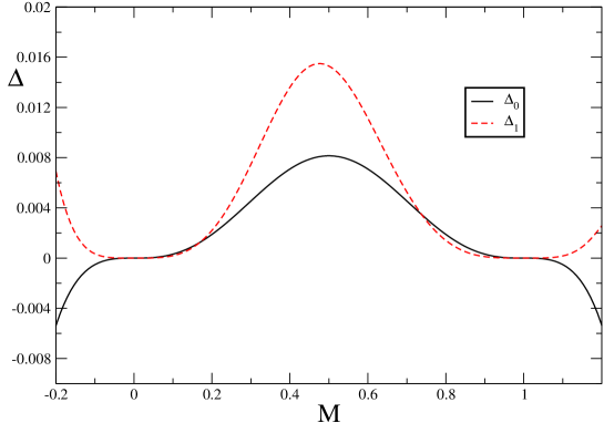
Figure 3: This plot shows the relative differences $\Delta=$ (exact-approximate)/exact for the leading order kernel ($\Delta_{0}$) and the next-to-leading kernel ($\Delta_{1}$).

4 Conclusions

We have discussed the collinear approximation of the BFKL kernel. Results on duality relations and factorisation schemes, with the inclusion of the running coupling enable us to construct an approximation of the BFKL kernel at NNLO, which contains all the singular contributions at $M=0$ and $M=1$. The collinear approximation of $\chi_{0}$ and $\chi_{1}$ are in excellent agreement with the full results and so our result for $\chi_{2}$ is also likely to be close to true result for the NNLO kernel in the region relevant at leading twist.

References

- [1] V. S. Fadin and L. N. Lipatov, Phys. Lett. B429, 127 (1998). hep-ph/9802290
- [2] R. D. Ball and S. Forte, Phys. Lett. B405, 317 (1997). hep-ph/9703417
- [3] G. Altarelli, R. D. Ball, and S. Forte, Nucl. Phys. B575, 313 (2000). hep-ph/9911273
- [4] A. Vogt, S. Moch, and J. A. M. Vermaseren, Nucl. Phys. B691, 129 (2004). hep-ph/0404111
- [5] G. P. Salam, Acta Phys. Polon. B30, 3679 (1999). hep-ph/9910492
- [6] R. D. Ball and p. Forte, Phys. Lett. B465, 271 (1999). hep-ph/9906222
- [7] G. Altarelli, R. D. Ball, and S. Forte, Nucl. Phys. B621, 359 (2002). hep-ph/0109178
- [8] R. D. Ball and S. Forte, Nucl. Phys. B742, 158 (2006). hep-ph/0601049
- [9] M. Ciafaloni, Phys. Lett. B356, 74 (1995). hep-ph/9507307
- [10] M. Ciafaloni and D. Colferai, JHEP 09, 069 (2005). hep-ph/0507106
- [11] S. Catani and F. Hautmann, Nucl. Phys. B427, 475 (1994). hep-ph/9405388
- [12] S. Marzani, R. D. Ball, P. Falgari, and S. Forte (2007). arXiv:0704.2404 [hep-ph]
- [13] M. Ciafaloni, D. Colferai, and G. P. Salam, JHEP 10 (1999)
- [14] V. Del Duca and E. W. N. Glover, JHEP 10, 035 (2001). hep-ph/0109028
- [15] J. Bartels and C. Bontus, Phys. Rev. D61, 034009 (2000). hep-ph/9906308.