µ m Å^-1

In-situ studies of bulk deformation structures:
Static properties under load
and
Dynamics during deformation
Ph.D. thesis by Bo Jakobsen (boj@ruc.dk)
 
Supervised by: Tage Emil Christensen (RUC),
Henning Friis Poulsen (Risø), & Wolfgang Pantleon (Risø) December 2006

Abstract

The main goal of the study presented in this thesis was to perform in-situ investigations on deformation structures in plastically deformed polycrystalline copper at low degrees of tensile deformation $(<5\%)$. Copper is taken as a model system for cell forming pure fcc metals.

A novel synchrotron-radiation based technique High Angular Resolution 3DXRD has been developed at the 1-ID beam-line at the Advanced Photon Source. The technique extents the 3DXRD approach, to 3D reciprocal space mapping with a resolution of $\approx 1\cdot 10^{-3}\rAA$ and allows for in-situ mapping of reflections from deeply-embedded individual grains in polycrystalline samples during tensile deformation.

We have shown that the resulting 3D reciprocal space maps from tensile deformed copper comprise a pronounced structure, consisting of bright sharp peaks superimposed on a cloud of enhanced intensity. Based on the integrated intensity, the width of the peaks, and spatial scanning experiments it is concluded that the individual peaks arise from individual dislocation-free regions (the subgrains) in the dislocation structure. The cloud is attributed to the dislocation rich walls.

Samples deformed to $2\%$ tensile strain were investigated under load, focusing on grains that have the tensile direction close to the $\left<100\right>$ direction. It was found that the individual subgrains, on average, are subjected to a reduction of the elastic strain with respect to the mean elastic strain of the grain. The walls are equivalently subjected to an increased elastic strain. The distribution of the elastic strains between the individual subgrains is found to be wider than the distribution of strains within the individual subgrains. The average properties are consistent with a composite type of model. The details, however, show that present understanding of asymmetrical line broadening have to be reconsidered.

Based on continuous deformation experiments, it is found that the dislocation patterning takes place during the deformation, and that a subgrain structure appears from the moment where plastic deformation is detected. By investigating samples under stress relaxation conditions, and unloading, it is found that the overall dislocation structure only depends on the maximum obtained flow stress. However, some changes in orientation and internal strain distribution between the subgrains were observed after the unloading.

An in-situ stepwise straining experiment of a pre-deformed sample was performed, allowing for investigation of individual subgrains during straining. The result indicates that the cell refinement process generally does not take place through simple subgrain breakups. Surprisingly, the dislocation structure shows intermittent behavior, with subgrains appearing and disappearing with increasing strain, suggesting a dynamical development of the structure.

Preface

This thesis is submitted in partial fulfilment of the requirements for obtaining the Ph.D. degree in physics at Roskilde University (RUC).

The research presented here was carried out within the Center for Fundamental Research: Metal Structures in Four Dimensions (M4D), at Risø National Laboratory. The studies were conducted during the period from January 2004 to December 2006.

My supervisors have been Tage Emil Christensen (RUC), Henning Friis Poulsen (M4D) and Wolfgang Pantleon (M4D), who all are thanked for their help and support throughout the project.

The experimental work was conducted at the 1-ID beam-line of the Advanced Photon Source (APS) at the Argonne National Laboratory, USA. The experiments would have been impossible without the close collaboration with our main contact at APS, Ulrich Lienert. He is warmly thanked for all his very valuable help, and for teaching me so much about experimental X-ray physics through all the long night shifts we shared.

Beside U. Lienert I had the opportunity to meet and work together with a number of very pleasant people at the APS: John Almer, Sarvjit D. Shastri, Ali Mashayekhi, Joel Bernier, and Dean Haeffner. I am very grateful for all their help, without which we could never have performed the experiments presented, and for making all my visits to APS very pleasant despite the workload.

Carsten Gundlach (M4D), Henning Osholm Sørensen (M4D), and Matthias Prinz (Freiberg University of Mining and Technology) are acknowledged for participating in beam times, and M. Prinz furthermore for doing some of the “data mining” for the Grain III dataset presented in section 4.2.

All electron microscopy investigations conducted in connection with this study have been done by the “microscopy and sample preparation experts” in the M4D group: Qingfeng Xing, Xiaoxu Huang, Gitte Christiansen, Preben Olesen, Helmer Nilson, and Guilin Wu. General preparation of the sample material was done by Palle Nielsen and Lars Lorentzen. They are all thanked for their very valuable help in producing and characterizing the sample material.

Brian Ralph (School of Engineering and Design, Brunel University, UK) and Rasmus Brauner Godiksen (M4D) took time for reading and commenting this thesis, for which I am deeply grateful.

The whole M4D group is thanked for making these 3 years very pleasant; especially the “227 office”; Tine Knudsen, Kristoffer Haldrup and Rasmus Brauner Godiksen with whom I have sheared most of my time at Risø.

Finally I would like to thank my long time colleague and friend Kristine Niss, and my wife Bodil Hjort Mynster for all the moral support that got me through the time as a Ph.D. student.

Bo Jakobsen

Risø, December 2006

Comment for arXiv/cond-mat version of the thesis

The originally submitted thesis included the six papers quoted as Paper I – Paper VI (see page Bibliography) as an appendix. Due to copyright issues the appendix has been omitted in this version, and minor changes has been applied to the main text accordingly. The thesis is meant to be self contained, but it is strongly advisable to also acquire the papers.

The thesis was successfully defended Marts 2007.

Bo Jakobsen

Roskilde University, August 2007

This work was supported by the Danish National Research Foundation and the Danish Natural Science Research Council.

Use of the Advanced Photon Source was supported by the U. S. Department of Energy, Office of Science, Office of Basic Energy Sciences, under Contract No. W-31-109-ENG-38.

A number of papers have been written in connection with this Ph.D. project, they are listed below.

B. Jakobsen, H. F. Poulsen, U. Lienert, J. Bernier, C. Gundlach, and W. Pantleon. Stability of dislocation structures in Cu towards strain relaxation. In preparation.

B. Jakobsen, U. Lienert, J. Almer, H. F. Poulsen, and W. Pantleon. Direct observation of strain in bulk subgrains and dislocation walls by high angular resolution 3DXRD. Materials Science and Engineering: A, 2007. Article in Press. doi:10.1016/j.msea.2006.12.168

B. Jakobsen, H. F. Poulsen, U. Lienert, X. Huang, and W. Pantleon. Investigation of the deformation structure in an aluminium magnesium alloy by high angular resolution three-dimensional X-ray diffraction. Scripta Materialia, 56:769–772, 2007.

B. Jakobsen, U. Lienert, J. Almer, W. Pantleon, and H. F. Poulsen. Properties and dynamics of bulk subgrains probed in-situ using a novel x-ray diffraction method. Materials Science Forum, 550:613–618, 2007.

B. Jakobsen, H. F. Poulsen, U. Lienert, and W. Pantleon. Direct determination of elastic strains and dislocation densities in individual subgrains in deformation structures. Acta Materialia, 55:3421–3430, 2007.

U. Lienert, J. Almer, B. Jakobsen, W. Pantleon, H. F. Poulsen, D. Hennessy, C. Xiao, and R. M. Sute. 3-dimensional characterization of polycrystalline bulk materials using high-energy synchrotron radiation. Materials Science Forum, 539–543:2353–2358, 2007.

W. Pantleon, B. Jakobsen, U. Lienert, J. Almer, C. Gundlach, and H. F. Poulsen. In-situ observation of individual subgrains by 3DXRD during deformation and recovery. In Proceedings of PLASTICITY ’06: The Twelfth International Symposium on Plasticity and its Current Applications, pages 664–666, 2006.

B. Jakobsen, H. F. Poulsen, U. Lienert, J. Almer, S. D. Shastri, H. O. Sørensen, C. Gundlach, and W. Pantleon. Formation and subdivision of deformation structures. Science, 312:889–892, 2006.

H. O. Sørensen, B. Jakobsen, E. Knudsen, E. M. Lauridsen, S. F. Nielsen, H. F. Poulsen, S. Schmidt, G. Winther, and L. Margulies. Mapping grains and their dynamics in three dimensions. Nuclear Instruments and Methods in Physics Research Section B, 246:232–237, 2006.

U. Lienert, J. Almer, B. Jakobsen, H. F. Poulsen, and W. Pantleon. Observation of dislocation structure evolution by analysis of X-ray peak profiles from individual bulk grains. In Proceedings of the 25th Risø International Symposium on Materials Science: Evolution of Deformation Microstructures in 3D, pages 417–422, 2004.

Dansk Resumé

Hovedformålet med det ph.d.-studie, som præsenteres i denne afhandling, er at foretage in-situ undersøgelser af dislokationsstrukturer i plastisk deformeret kobber ved små deformationsgrader $(<5\%)$. Kobber skal i denne sammenhæng ses som et modelmateriale for de rene fcc metaller, hvor dislokationerne arrangerer sig i en celle-struktur.

Vi har udviklet en synkrotronbaseret røntgenteknik (High Angular Resolution 3DXRD), som tilføjer højopløst 3D kortlægning af det reciprokke rum til rækken af 3D røntgendiffraktionsteknikker (3DXRD teknikker). Udviklingen af teknikken er foregået på 1-ID beam-linjen på synkrotronen Advanced Photon Source ved Argonne National Laboratory, USA. Metoden gør det muligt at undersøge forbreddede Bragg refleksioner fra dybtliggende individuelle korn i en polykrystal, og det med en opløsning på $\approx 1\cdot 10^{-3}\rAA$. Videre er tidsopløsningen god nok til, at man er i stand til at følge strukturudviklingen in-situ under deformation.

Vi har fundet, at sådanne 3D kort over Bragg refleksioner fra plastisk deformeret kobber indeholder en udtalt struktur bestående af skarpe toppe med høj intensitet overlejret på en sky af forholdsvis lav intensitet. Den integrerede intensitet i og bredden af disse toppe samt den rumlige fordeling af materialet, som giver anledning til disse, er blevet analyseret. På den baggrund konkluderer vi, at toppene er diffraktionssignalet fra de individuelle dislokationsfrie områder i strukturen (underkornene). Tilsvarende konkluderer vi, at skyen stammer fra de dislokationsfyldte vægge, som separerer underkornene.

Underkornene i plastisk deformeret metal er traditionelt blevet undersøgt med transmissionselektronmikroskopi, som er en destruktiv teknik, eller med klassiske røntgenteknikker, som midler over mange underkorn. “High Angular Resolution 3DXRD” teknikken giver mulighed for direkte og med rimelig tidsopløsning at undersøge egenskaberne af underkorn dybt inde i et korn.

Den interne fordeling af elastisk tøjning blev undersøgt i prøver deformeret til $2\%$ forlængelse. Specielt fokuserede vi på korn, hvor trækretningen er tæt på en $\langle 100\rangle$ krystallografisk retning. Det blev fundet, at underkornene i gennemsnit er udsat for en reduceret elastisk tøjning i forhold til den gennemsnitlige elastiske tøjning i kornet. Det blev tilsvarende fundet, at væggene er udsat for en forhøjet elastisk tøjning. Analysen viste desuden, at fordelingen af elastisk tøjning mellem underkornene er bredere end fordelingen af elastisk tøjning, som findes internt i de enkelte underkorn.

Disse resultater peger på, at komposit-modeller for dislokationsstrukturen beskriver den gennemsnitlige fordeling af elastisk tøjning korrekt. Resultaterne viser imidlertid også, at den nuværende forståelse af asymmetrisk-forbreddede røntgen-linjeprofiler skal revideres, da man i eksisterende analysemetoder antager, at tøjningsfordelingen mellem underkornene er meget smallere end den interne tøjningsfordeling.

Et andet resultat af målingerne er, at tætheden af dislokationer i underkornene er meget lille. Tætheden af redundante dislokationer er mindre end $12\cdot 10^{12}\mathrm{m}^{-2}$. Vi har desuden fundet, at teknikken kan være følsom for ned til én uparret dislokation.

Prøver er også blevet undersøgt under kontinuerlig deformation både fra fuldt udglødet tilstand og fra pre-deformeret tilstand. Ved at følge en Bragg refleks fra et korn under deformation fandtes, at dislokationsstrukturen opstår og udvikler sig kontinuerligt under deformationen, og at underkornsstrukturerne eksisterer fra det øjeblik, hvor den plastiske deformation er detekterbar. Ved tilsvarende undersøgelser, hvor spændinger blev relakseret og prøven aflastet, fandtes, at den overordnede dislokationsstruktur udelukkende afhænger af den maximalt opnåede flydespænding. Under aflastning sås dog ændringer i tøjnings- og orienteringsfordelingen mellem underkornene.

En pre-deformeret prøve blev undersøgt under trinvis deformation. Sådanne forsøg tillader, at man undersøger udviklingen af individuelle underkorn som funktion af tøjning. Resultaterne indikerer, at underkorn ikke deler sig gennem en simpel opbygning af nye vægge. De ser ud til at opstå og forsvinde dynamisk, mens prøven deformeres. Hvis dette resultat kan eftervises ved højere deformationsgrader, kan det f.eks. give en forklaring på, hvordan dislokationsvægge opretholder en foretrukken orientering under deformation.

De opnåede resultater kan forhåbentlig inspirere til nye modeller for deformationshærdning og strukturformation i metaller.

List of commonly used notations

$\lx@intercol\bm{q}\hfil$	Scattering vector. Normally expressed in the defined q-space coordinate system
$\lx@intercol\theta\hfil$	Scattering angle
$\lx@intercol\theta_{0}\hfil$	Scattering angle for an undeformed perfect sample
$\lx@intercol\eta\hfil$	Azimuthal angle
$\lx@intercol\omega,\phi,\chi\hfil$	Available rotations on the setup
$\lx@intercol\Delta\omega\hfil$	Rocking interval
$\lx@intercol\bm{q}_{x},\bm{q}_{z},\bm{q}_{z}\hfil$	Basic vectors for the reciprocal space coordinate system
$\lx@intercol\bm{x},\bm{y},\bm{z}\hfil$	Basic vectors for the laboratory coordinate system
$\lx@intercol(\bm{a},\bm{b})\hfil$	Plane spanned by the two vectors $\bm{a}$ and $\bm{b}$
$\lx@intercol\left[uvw\right]\hfil$	Lattice vector in crystallographic coordinates
$\lx@intercol\langle uvw\rangle\hfil$	Lattice vector family
$\lx@intercol(hkl)\hfil$	Lattice plane with Miller index $hkl$
$\lx@intercol\{hkl\}\hfil$	Lattice plane family with Miller index $hkl$
$\lx@intercol hkl\hfil$	Reflection (or reflection family) from lattice plane (hkl) (or lattice plane family $\{hkl\}$)
$\lx@intercol E\hfil$	Energy of the X-ray beam
$\lx@intercol\lambda\hfil$	Wavelength of the X-ray beam.
$\lx@intercol L\hfil$	Horizontal sample-to-detector distance.
$\lx@intercol\bm{a}_{1},\bm{a}_{2},\bm{a}_{3}\hfil$	Crystal lattice basic vectors
$\lx@intercol\bm{a}^{*}_{1},\bm{a}^{*}_{2},\bm{a}^{*}_{3}\hfil$	Reciprocal lattice basic vectors

Sketch of the setup, defining axes in real and reciprocal space, rotation angles and scattering angles. For full figure text see page 3.7.

Contents

1. 1 Introduction
   1. 1.1 Deformation structures in metals
      1. 1.1.1 Dislocations
      2. 1.1.2 Phenomenology of dislocation structures in copper
      3. 1.1.3 Techniques for investigating dislocation structures
      4. 1.1.4 Open questions
   2. 1.2 Development of the project
2. 2 Background
   1. 2.1 Basic scattering theory
   2. 2.2 Diffraction from a perfect crystal
   3. 2.3 Diffraction from real crystals
      1. 2.3.1 Quantitative analysis of broadened reflections
   4. 2.4 Experimental investigation of diffraction
      1. 2.4.1 The rotation method
      2. 2.4.2 The powder method
      3. 2.4.3 Investigation of intensity distributions
   5. 2.5 Recent developments
      1. 2.5.1 3DXRD microscopy
      2. 2.5.2 The 3D crystal microscope
      3. 2.5.3 3DXRD peak shape analysis
3. 3 High Angular Resolution 3DXRD
   1. 3.1 Overview
      1. 3.1.1 The technique
      2. 3.1.2 Interpretation of data
      3. 3.1.3 Samples
   2. 3.2 The setup at 1-ID (APS)
      1. 3.2.1 Optics and beam monitoring
      2. 3.2.2 Stress rig
      3. 3.2.3 Euler cradle
      4. 3.2.4 Detectors
   3. 3.3 Selecting grains and reflections
      1. 3.3.1 Reflection-based selection of a grain
      2. 3.3.2 Grain-based selection of reflections
      3. 3.3.3 Ensuring that a grain is in the bulk
   4. 3.4 Reciprocal space mapping
      1. 3.4.1 Data collection
      2. 3.4.2 Definition of the reciprocal space coordinate system
   5. 3.5 Instrumental resolution
      1. 3.5.1 Relations between experimental parameters and resolution
      2. 3.5.2 Calculated instrumental resolution
      3. 3.5.3 Measured instrumental resolution
   6. 3.6 Data analysis
      1. 3.6.1 First order rebinning
      2. 3.6.2 Projections of reciprocal space
      3. 3.6.3 Single peak analysis
      4. 3.6.4 Statistical analysis of intensity distribution
      5. 3.6.5 Volume calibration
   7. 3.7 Reproducibility
   8. 3.8 Detailed arguments for the interpretation
      1. 3.8.1 Observations from raw data
      2. 3.8.2 Single peaks
      3. 3.8.3 The diffuse cloud
   9. 3.9 Comparison to other techniques
4. 4 Results and discussion
   1. 4.1 Introduction
   2. 4.2 Distribution of elastic strain
   3. 4.3 Dislocation density in the subgrains
   4. 4.4 Formation and stability of subgrains
      1. 4.4.1 Formation of dislocation structures
      2. 4.4.2 Stability of dislocation structures
   5. 4.5 Subgrain refinement
5. 5 Conclusions and outlook
6. Bibliography

Chapter 1 Introduction

This thesis deals with the fundamental properties of dislocation structures that evolve in metals as they are plastically deformed.

There are, at least, two reasons why such structures are interesting. Firstly, they are an example of natural pattern formation which has a range of unexplained phenomena associated. Secondly the structures have an influence on the properties of metals, and are hence interesting from an applied perspective. The first point is what is important to me, and I will not in this thesis discuss the consequences of the results in an applied framework.

Two main issues have been investigated:

• What are the static properties of the dislocation structures under load?

• What are the dynamics of the structures during deformation?

The main focus has been on pure fcc metals, and the model material of choice is polycrystalline copper (Cu), which has been investigated in great details in the past. The deformation mode has been restricted to tensile deformation. Mainly small plastic deformations (in the range of $0-5\%$) have been considered, as the focus is on the creation of deformation structures and their properties in the initial phase of structure formation. Focus has further been on grains where the tensile axis is close to the crystallographic $\left<100\right>$ direction.

A major part of my work has been devoted to the development of a novel technique: “High Angular resolution 3DXRD”. The method is based on 3D reciprocal space mapping of individual reflections from individual bulk grains in polycrystalline samples. By means of a setup developed at the 1-ID beam line of the Advanced Photon Source (APS) at the Argonne National Laboratory, USA, such 3D maps can be acquired in-situ and reasonably fast. These maps turn out to provide access to direct information on the deformation structure. The contents of the thesis reflects this experimental development.

This thesis is divided into four major chapters:

Chapter 1:

Beside this short introduction, the present chapter includes an introduction to deformation structures in metals, the techniques used to investigating them, and the questions that I have touched upon in this study. This is followed by a brief overview of my Ph.D. project.

Chapter 2:

Gives an overview of the background of my work. This includes diffraction theory for deformed and undeformed metals, and classical X-ray methods for investigating such diffraction signals (section 2.1 to 2.4). Section 2.5 discusses some of the recent developments in synchrotron-based techniques, two of which this work is based on.

Chapter 3:

Gives a thorough description of High Angular resolution 3DXRD. The chapter provides a detailed description of the setup, data analysis and arguments for interpretation. Finally the technique is compared with other techniques.

Chapter 4:

The major scientific results of my study is presented in a number of papers (science–newdyn). Chapter 4 gives an overview of the results, connecting results presented in different publications and presents some yet unpublished results.

Conclusions and outlook are finally presented in chapter 5.

References to the major publications are throughout this thesis designated as science–newdyn, accordingly to the list presented first in the bibliography.

1.1 Deformation structures in metals

The plastic deformation of metals is carried by the movement of line defects, dislocations, through the crystal.

During the propagation of the dislocations, some of them will be trapped in the crystal. The trapping can be due to e.g. foreign particles in the crystals, but stems mainly from interaction between individual dislocations.

It is well known that the dislocations stored in a crystal have a tendency to self organize into ordered structures, known as dislocation structures or deformation structures. The morphology of the structures formed depends on the material investigated, the mode of deformation, and the degree of deformation.

An introduction to dislocations and dislocation structures will be presented in the following. The focus will be on the material of choice, copper, but the results presented are general for a large class of pure fcc materials (for a general review of deformation structures see e.g. [hansen2004_handbook]).

1.1.1 Dislocations

A vast amount of literature exists on dislocation theory including a number of very good text-books such as [Weertman1964] and [Hull1984], for a general introduction to the concept please refer to one of these.

Figure 1.1: Left) Atomic positions around an edge dislocation in a simple cubic (sc) crystal. The positions are calculated from the continuum displacement field for one edge dislocation in an infinite crystal (as e.g. found in [Weertman1964]). The position of the dislocation is indicated by the red symbol. A Burgers circuit around the dislocation is shown (blue line). Elastic properties of copper were used in the calculation, and the Burgers vector set to one inter-atomic distance. Right) Equivalent Burgers circuit in a perfect crystal. The corresponding Burgers vector is indicated by the red arrow.

The left part of figure 1.1 shows the distorted atomic lattice around one dislocation. A Burgers circuit is drawn around the dislocation. In the right part of the figure the corresponding circuit is shown in a perfect crystal, and the resulting closure failure shown; this is the Burgers vector of the dislocation. Dislocations are beside the Burgers vector characterized by their direction. Dislocations are separated into edge, screw and mixed dislocations. Edge and screw dislocations have Burgers vector perpendicular and parallel to the direction of the dislocation respectively, and a mixed dislocation an intermediate angle. It is in figure 1.1 seen that the lattice is rather perfect far from the dislocation, and that a shear deformation is created if the dislocation is moved completely through the lattice.

Dislocations give rise to displacement of the crystalline material around them. The description of a dislocation is normally divided into a part describing the “core” of the dislocation, that is the atoms very close to the dislocation, and a part describing the displacement of the crystal further away from the dislocation.

Elasticity theory can be applied away from the dislocation core. Such elastic descriptions which gives the displacement, stress, and strain fields around the dislocation, exists for multiple dislocation types and boundary conditions (see e.g. [leibfried49] and the general discussion in e.g.
[Weertman1964]).

An interesting and general feature of the stress/strain fields of a dislocation is that they are long-ranged. They go to zero as $1/r$ ($r$ being the distance from the dislocation). This has the consequence that the elastic energy of a dislocation generally increases logarithmically with the size of the crystal, and therefore diverges.

Figure 1.2: A) Symmetrical tilt boundary with dislocation spacing $D$ and tilt angle $\beta$. B) dislocation dipole.

Dislocations can be arranged in a number of stable configurations, with lower energy than a single dislocation. Figure 1.2 show two examples of such structures, the symmetrical tilt boundary and the dislocation dipole. The stress field of the symmetrical tilt boundary goes down as fast as $e^{-r}$, and the dipole field as $1/r^{2}$. The tilt boundary has the property that the crystal parts on each side are rotated with respect to each other. The angular difference between the two sides, $\beta$ is given as $\beta=b/D$ with $b$ the length of the Burgers vector and $D$ the spacing between the dislocations.

An interesting configuration of dislocations is a spatially random distribution of dislocations, having an equal number of dislocations of opposite Burgers vector. It can be shown that the elastic energy for such a distribution also diverges logarithmically with the size of the crystal [Wilkens1970c; Wilkens1984].

Hence in order to lower the energy the dislocations stored in a crystal have to be arranged in ordered structures.

1.1.2 Phenomenology of dislocation structures in copper

The deformation structures in copper after tensile deformation have been investigated in great detail by electron microscopy over the last 40 years on both single crystals (to name a few: [Essmann1963; Steeds1966; Gottler1973; Kawasaki1980; Wilkens1987]) and polycrystals (e.g. [essmann68; Huang1998]).

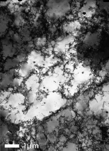
Figure 1.3: Transmission electron microscope image of $99.99\%$ pure OFHC Cu, deformed in tension to a plastic strain of $2\%$ (from [ science]).

It is generally found that the dislocations self organize into regions of relatively low dislocation density, knows as cell interiors or subgrains, separated by regions of much higher dislocation density, known as cell walls or subgrain boundaries. An example, in the form of an electron micrograph, of such a structure is shown in figure 1.3. The cell walls seen in the micrograph are rather loose, as the sample was only strained to $2\%$ tensile deformation. At higher plastic deformation the walls becomes sharper.

This separation into cells and cell walls are general for a large class of materials known as cell-forming metals (e.g. Al and Ni). For a general review of deformation structures see e.g. [Hansen1999; hansen01; hansen2004_handbook].

The morphology of the dislocation structure does, as mentioned earlier, depend on the deformation mode, but even with the same deformation mode large differences may exist. In the case of unidirectional tensile deformation it is found that the morphology depends on the direction of the tensile axis with respect to the crystallographic orientation of the crystal, with equivalent behavior for single crystals and grains in polycrystals. See [huang97; Huang1998] for work on polycrystals and references therein for work on single crystals.

In the general case the structure is hierarchal, consisting of what is known as cell blocks which again is separated into cells. The cell blocks are separated by boundaries of a rather high misorientation, whereas the cells are separated by boundaries of low misorientation [Kuhlmann-Wilsdorf1991].

In my work, I have focused on crystals which have a $\left<100\right>$ direction close to the tensile axis. The morphology in this case consists of equiaxed cells separated by cell boundaries as the one seen in figure 1.3 (see e.g. [Gottler1973]).

A very pronounced feature of the dislocation structure is that the length scale decreases with increasing plastic strain, a phenomenon known as cell refinement (see e.g. the classic work by Gottler1973). The misorientation between the cells furthermore increases with increasing plastic strain (e.g. [Hughes1997a; Pantleon2002]).

The underlying principles controlling the structural formation have been a matter of debate over the last many years. Two main ideas exist on why structures form: lowering of energy (Low Energy Dislocation Structure (LEDS)), and self organization. In the case of LEDS theory it is argued that the dislocations will form structures that among the available conformations lead to a minimization of the free energy (e.g. [kuhlmann-wilsdorf01]). Self organization theories are based on the general observation that driven systems far from equilibrium have a natural tendency to form structures (e.g. [Seeger1988]). For a detailed discussion of different models see the comprehensive review by kubin92MatSciTec.

However, it seems to be generally accepted that dislocations need to be mobile in three dimensions [Kuhlmannwilsdorf1994; madec02Scripta; hansen2004_handbook] for structural formation to exist. This has the consequence that properties such as stacking fault energy and alloying elements change the structure formation ability of a metal.

1.1.3 Techniques for investigating dislocation structures

Classically two main methods are used for the investigation of dislocation structures; transmission electron microscopy (TEM) and X-ray line profile analysis.

Transmission electron microscopy

Transmission electron microscopy is by far the most commonly used technique for investigating dislocation structures. The technique gives very informative real-space images of the dislocation structures but has some disadvantages, mainly related to the fact that thin films have to be prepared for investigation:

• Care has to be taken to hinder relaxation of dislocation structures and internal strain distribution during sample preparation.
  See e.g. [Essmann1963; Young1967; Crump1968; Mughrabi1971]

• It is impossible to investigate bulk samples under tensile deformation.
  See e.g. [Myshlyaev1978] for an example of creep investigations performed on thin films, and [Martin1978] for a discussion of the limitation of in-situ studies by high voltage TEM.

Traditional X-ray techniques

Alternately; characterization can be performed with X-ray techniques, especially line profile analysis and rocking curve analysis (see e.g. [Wilkens1970; Wilkens1987; Warren1950; Ungar1984; Krivoglaz1996]). Further detains on some of these techniques are provided in section 2.3.1.

The methods will give information on average properties such as strain distribution, dislocation density and orientation distribution. The main advantage is that the techniques are non-destructive. The techniques are on the other hand highly indirect as:

• The results represent the average over many structural elements (subgrains and in the case of polycrystalline samples also grains). These elements will have one common direction of the lattice plane normal, but have different crystallographic orientations in the sample and different neighboring environments.

• Models are needed to interpret the results. The use of such models introduces additional assumptions which often can be hard to verify by independent experiments.

Recent X-ray methods

The availability of synchrotron radiation has lead to the development of new methods. Most interesting for the present work are the 3D X-ray diffraction (3DXRD) microscope [poulsen04:bog], and the 3D X-ray crystal microscope [Larson2002] (described in section 2.5.1 and 2.5.2).

Both techniques do however have some limitations:

• The 3DXRD microscope does not have the spatial resolution for direct observation of the deformation microstructure.

• The 3D X-ray crystal microscope is based on a spatial scanning technique, which limits the volume that can be mapped in a feasible time.

1.1.4 Open questions

Fundamental questions on deformation structures exist even though they have been investigated intensively over the last many years. During my work I have touched upon a few of such questions:

• What is the elastic strain in the subgrains and subgrain walls?
  (section 4.2)

• What is the dislocation density in the subgrains?
  (section 4.3)

• When do the dislocation structures form?
  (section 4.4.1)

• What is the stability of dislocation structures?
  (section 4.4.2)

• How does the cell refinement take place?
  (section 4.5)

1.2 Development of the project

A close interlink exists between the questions dealt with, and the development of High Angular Resolution 3DXRD.

The original plan for the Ph.D. project was to use “3DXRD peak shape analyse” (see section 2.5.3) for in-situ investigations of the dynamical properties of dislocation structures. Such a study would have been rather simple from an experimental perspective, as the technique already existed. As for many other X-ray techniques it would have required a heavy use of models for interpreting the data.

However, during one of the very first beam-time experiments we discovered that it might be possible to obtain diffraction signals from individual subgrains in a deformed structure.

Based on these first indications, with the experiments conducted on thin films and on polycrystalline aluminum samples, it was decided to use more beam-time on exploring these possibilities. In close collaboration with U. Lienert (our local collaborator at APS) it was decided to change the X-ray optics completely with respect to what had been used before. This new X-ray optics setup allowed for reasonable data acquisition times and high angular resolution at the same time.

Based on the data acquired it was confirmed that we were able to obtain in-situ diffraction data directly from individual subgrains embedded in a bulk grain in a polycrystalline sample.

With the technique established a range of questions came to mind which might be possible to investigate in a more direct way than previously had been possible. This included the questions on subgrain dynamics which was the initial goal, but also questions regarding the internal strain distribution in the grain and the consequences for line profile analysis.

Chapter 2 Background

The relevant basic diffraction theory and general experimental methods will be briefly reviewed in this chapter.

It should not be seen as a general introduction to diffraction, for this I refer to the large number of text books on this subject, such as [Guinier1963], [warren1969] and [Als-Nielsen2001].

2.1 Basic scattering theory

General scattering theory will be described in the following section. The theory will be restricted to kinematic scattering in the elastic limit of monochromatic X-rays, as these are the relevant conditions for the present study.

An object consisting of a number of atoms is shown in figure 2.1. The scattering ability of the individual atoms is described by the atomic scattering factor, $f_{j}$, and the position by the vector, $\bm{r}_{j}$.

The object is illuminated by a plane wave monochromatic X-ray beam described by the wave vector $\bm{k}_{0}$. The scattered wave is observed at the point, $O$. This observation point is assumed to be far away from the object relative to the size of the object, therefore the scattered waves from the different atoms can be described by the same wave vector $\bm{k}$. The length of the wave vector is preserved due to the assumption of elastic scattering, that is:

$$|\bm{k}|=|\bm{k}_{0}|=\frac{2\pi}{\lambda}$$ (2.1)

where $\lambda$ is the wavelength of the X-ray beam.

Figure 2.1: A general ensemble of atoms. The scattering ability of the $j$’th atom is described by the atomic scattering factor for that atom, $f_{j}$, and its position by the vector $\bm{r}_{j}$. $\bm{k}_{0}$ is the wave vector of the incoming monochromatic beam, and $\bm{k}$ is the wave vector of the scattered beam as observed from the point $O$. It is assumed that the distance from the ensemble of atoms to the observer is much larger than the dimensions of the collection that is: $|\bm{O}-\bm{r}_{i}|\gg|\bm{r}_{j}-\bm{r}_{k}|\forall i,j,k$.

The scattering property of such an object is described by the complex scattering amplitude, $A$, which describes both the amplitude and the phase of the observed scattered wave relative to the incoming wave. The phase difference, in the scattered waves, due to the different positions of the atoms can be found as:

$$(\bm{k}-\bm{k}_{0})\cdot\bm{r_{j}}=\bm{q}\cdot\bm{r_{j}},$$ (2.2)

with the scattering vector, $\bm{q}$, defined as $\bm{q}=\bm{k}-\bm{k}_{0}$.

The scattering amplitude from a collection of atoms can be written as:

$$A(\bm{q})=\sum_{j}f_{j}(\bm{q})e^{i\bm{q}\cdot\bm{r}_{j}},$$ (2.3)

where $f_{j}(\bm{q})$ is the $\bm{q}$-dependent atomic scattering factor for atom $j$.

However, X-ray detectors do not record both the phase and the amplitude of the scattered beam, but only the intensity, $I(\bm{q})$, which is given as:

$$I(\bm{q})=AA^{*}=|A(\bm{q})|^{2};$$ (2.4)

hence the phase information is lost.

2.2 Diffraction from a perfect crystal

The crystal lattice

The position of the atoms in a crystalline material is normally described by a lattice and a basis.

A crystal lattice is characterized by the fact that it obeys certain translation symmetries. A 3D lattice can be described by three crystal lattice basis vectors, $\bm{a}_{1}$, $\bm{a}_{2}$ and $\bm{a}_{3}$, which have the property that the lattice looks the same if translated by an integer number of any of these.

The lattice is more formally described by vectors in the form:

$$\bm{R}_{\bm{n}}=n_{1}\bm{a}_{1}+n_{2}\bm{a}_{2}+n_{3}\bm{a}_{3},$$ (2.5)

with $\bm{n}=(n_{1},n_{2},n_{3})$ all being integers.

These vectors give the position of the unit cells of the crystal, the lattice points, each unit cell is populated by the same arrangement of atoms described by what is known as the basis. In total:

$$\text{lattice}+\text{basis}=\text{crystal structure}.$$ (2.6)

The choice of crystal lattice basis vectors is not unique, nor is the basis.

The basis can be described by vectors, $\bm{r}_{j}$, relative to the lattice points. The position of any given atom in a crystal can be given as:

$$\bm{R}_{\bm{n},j}=\bm{R}_{\bm{n}}+\bm{r}_{j}=n_{1}\bm{a}_{1}+n_{2}\bm{a}_{2}+n_{3}\bm{a}_{3}+\bm{r}_{j},$$ (2.7)

for some $\bm{n},j$.

Scattering amplitude

The general formula for the scattering amplitude (equation 2.3) can in the case of a crystal be separated into two parts as:

$$A(\bm{q})=\sum_{\bm{n},j}f_{j}(\bm{q})e^{i\bm{q}\cdot\bm{R}_{\bm{n},j}}=\overbrace{\sum_{j}f_{j}(\bm{q})e^{i\bm{q}\cdot\bm{r}_{j}}}^{\text{unit cell sum}}\overbrace{\sum_{\bm{n}}e^{i\bm{q}\cdot\bm{R}_{\bm{n}}}}^{\text{lattice sum}},$$ (2.8)

where the “unit cell sum” is the sum over the atom configuration in the basis, and the “lattice sum” is over all lattice points.

The reciprocal space and lattice

In the description of diffraction it turns out to be very useful to construct what is known as reciprocal space.

The reciprocal space is spanned by the reciprocal basis vectors, $\bm{a}_{1}^{*}$, $\bm{a}_{2}^{*}$, and $\bm{a}_{3}^{*}$. These basis vectors are related to the crystal lattice basis vectors by:

$$\bm{a}_{1}^{*}=\frac{2\pi}{v_{c}}\bm{a}_{2}\times\bm{a}_{3},\quad\bm{a}_{2}^{*}=\frac{2\pi}{v_{c}}\bm{a}_{3}\times\bm{a}_{1},\quad\bm{a}_{3}=\frac{2\pi}{v_{c}}\bm{a}_{1}\times\bm{a}_{2},$$ (2.9)

with $v_{c}=\bm{a}_{1}\cdot(\bm{a}_{2}\times\bm{a}_{3})$ the volume of the unit cell. It can be seen that the dimension of the reciprocal lattice vectors are reciprocal in length, hence the name.

The two sets of basis vectors have the property that:

$$\bm{a}_{i}\cdot\bm{a}^{*}_{j}=2\pi\delta_{ij},$$ (2.10)

where $\delta_{ij}$ is the Kronecker delta.

In the cubic case we have $\bm{a}_{j}^{*}\parallel\bm{a}_{j}$, and $|\bm{a}_{j}^{*}|=\frac{2\pi}{|\bm{a}_{j}|}$. It is important to notice that the reciprocal space is tightly bound to the crystal. If the crystal is rotated so is the reciprocal space.

The reciprocal basis vectors span, in a natural way, a lattice in reciprocal space, with a reciprocal lattice vector, $\bm{G}$, given as

$$\bm{G}_{hkl}=h\bm{a}_{1}^{*}+k\bm{a}_{2}^{*}+l\bm{a}_{3}^{*},$$ (2.11)

with $h,k,l$ integers.

Reciprocal lattice vectors have the following properties, relating them to the underlying crystal structure:

• $\bm{G}_{hkl}$ is perpendicular to the lattice plane with Miller indices $hkl$.

• $|\bm{G}_{hkl}|=\frac{2\pi}{d_{hkl}}$, where $d_{hkl}$ is the lattice spacing of the lattice planes with Miller indices $hkl$.

The Laue condition

The scattering vector can be described in coordinates of the reciprocal space in a natural way:

$$\bm{q}=q_{1}\bm{a}_{1}^{*}+q_{2}\bm{a}_{2}^{*}+q_{3}\bm{a}_{3}^{*},$$ (2.12)

with $q_{1}$, $q_{2}$ and $q_{3}$ real dimensionless numbers.

The product $\bm{q}\cdot\bm{R}_{\bm{n}}$ in equation 2.8 then becomes:

$$\bm{q}\cdot\bm{R}_{\bm{n}}=2\pi(n_{1}q_{1}+n_{2}q_{2}+n_{3}q_{3}),$$ (2.13)

using equation 2.10.

In the case where $\bm{q}$ is a reciprocal lattice vector, this sum reduces to an integer times $2\pi$. The lattice sum in equation 2.8 then equals the number of lattice points (a large number) whereas it is of the order of unity in all other cases.

This is the Laue condition for observation of X-ray diffraction .

$$\bm{q}=\bm{G}$$ (2.14)

When investigating the diffracted intensity as function of the scattering vector, a detectable signal is only obtained when the Laue condition is fulfilled. Such maxima are normally termed Bragg peaks or reflections. The measured intensity, in the individual reflection from a crystal, is determined by the unit cell sum for the crystal.

2.3 Diffraction from real crystals

The description in the previous section is based on a perfect infinite crystal, somewhat different from the crystals investigated in reality. The lattice sum will be non zero in some region around the theoretical reciprocal lattice point if the crystal has e.g. a finite size, a distribution of lattice spacings or a distribution of lattice plane orientations; the reflection is said to be broadened.

The idea of many diffraction-based methods is to investigate such broadened reflections, and thereby obtain information on the material.

As a crystal is deformed, the lattice structure becomes distorted. This can mainly happen in two ways: the lattice plane spacing can change, and the orientation of the lattice planes can change. A crystal will after plastic deformation generally contain a distribution of lattice plane spacings and orientations, the latter sometimes termed the mosaic spread.

From the two main properties of the reciprocal lattice vectors (as stated on previous page) it is known that the length of a reciprocal lattice vector is related to the lattice plane spacing of the crystal, and that the orientation of the reciprocal lattice vector is related to the orientation of the crystal lattice planes.

A uniform straining of a crystal will hence lead to a radial shift, that is along the reciprocal lattice vector, of the reflection. An uniform rotation will equivalently lead to an azimuthal shift, that is perpendicular to the reciprocal lattice vector, of the reflection.

A distribution of lattice plane spacings (equivalently elastic strains) will give rise to a broadening of the intensity distribution in the radial direction. The distribution of orientations of lattice planes, will on the other hand give a broadening of the intensity distribution in the azimuthal directions. [Wilkens1984]

The broadening is easy to understand if the crystal is thought of as consisting of a number of incoherently scattering domains, each with some strain and orientation. In this case one can think of the broadened reflection as being the simple superposition, in intensity, of a large number of reflections. The peak shape will in such a case be related, in a simple way, to the distribution of strains and orientations among the domains. However, a plastically deformed metal can in the general case not be divided into such incoherently scattering domains with a well-defined strain and orientation, hence more elaborate models are needed taking into account the full distributions.

2.3.1 Quantitative analysis of broadened reflections

A few quantitative results regarding the broadening of reflections will be discussed in the following.

Broadening due to the finite size of the crystals

Beside broadening due to strain and orientation the reflections will also be broadened because of the finite site of the crystals.

Following the derivation by Krivoglaz1996 (originally formulated by Ewald1940) the general expression for the scattering amplitude (equation 2.8) can be reformulated as:

$$A(\bm{q})=\sum_{j}f_{j}(\bm{q})e^{i\bm{q}\cdot\bm{r}_{j}}\int Y^{\infty}(\bm{r})s(\bm{r})e^{i\bm{q}\cdot\bm{r}}d\bm{r},$$ (2.15)

where $Y^{\infty}$ describes the position of unit cells in a infinite large crystal, and $s(\bm{r})$ is a function which is $1$ inside the actual crystal and $0$ outside.

It is shown that the shape of the intensity distribution close to a reciprocal lattice point, $\bm{G}$, is given by:

$$I_{\text{Size}}(\bm{q})\propto|\tilde{s}(\bm{q}-\bm{G})|^{2},$$ (2.16)

where $\tilde{s}$ is the Fourier transform of $s$, and the unit cell sum has been neglected.

In the case of an infinite crystal we have $s=1$ for all space and $\tilde{s}(\bm{x})=\delta(\bm{x})$, (with $\delta(\bm{x})$ being the Dirac delta function), equation 2.16 hence reduces to the exact Laue condition as expected.

The width of the size-broadened peak, $\Delta q$, in some direction in reciprocal space, is related to the real-space length scale, $l$, of the crystal in the same real-space direction by:

$$\Delta q=k\frac{2\pi}{l}.$$ (2.17)

where $k$ is the Scherrer constant, which is related to the precise measure of the peak width, and the shape of the crystal (for a review of Scherrer constant in different cases see [Langford1978]). The Scherrer is generally not far from unity, it may for example be shown that $k=0.88$ for a box shaped crystal and a width-measure of full width at half maximum.

Strain broadening

It is general for classic formulations of strain broadening that they relate the azimuthally integrated radial peak profile of the reflection to some description of the strain distribution in the crystal. The reason for studying such integrated radial peak profiles is that they can easily be obtained from single crystals and powders with conventional diffractometers.

The derivations below follow Warren and Averbach as described in
[Warren1950] and [warren1969].

The deformation is assumed to be so smooth that the individual unit cells in the deformed crystal are equal (hence it makes sense to talk about a unit cell sum). The unit cell sum will in the following, without loss of generality be set to $1$.

The general equation for the diffracted intensity (equation 2.4) can be rewritten as:

$$I(\bm{q})=\sum_{\bm{n}}e^{i\bm{q}\cdot\bm{R}_{\bm{n}}}\sum_{\bm{n}^{\prime}}e^{-i\bm{q}\cdot\bm{R}_{\bm{n}^{\prime}}}=\sum_{\bm{n}}\sum_{\bm{n}^{\prime}}e^{i\bm{q}\cdot(\bm{R}_{\bm{n}}-\bm{R}_{\bm{n}^{\prime}})}.$$ (2.18)

The position of the unit cells in a distorted crystal can be described by:

$$\bm{R}_{\bm{n}}=n_{1}\bm{a}_{1}+n_{2}\bm{a}_{2}+n_{3}\bm{a}_{3}+(\delta_{1}(\bm{n})\bm{a}_{1}+\delta_{2}(\bm{n})\bm{a}_{2}+\delta_{3}(\bm{n})\bm{a}_{3}),$$ (2.19)

where $\bm{\delta}(\bm{n})=(\delta_{1}(\bm{n}),\delta_{2}(\bm{n}),\delta_{3}(\bm{n}))$ is a small perturbation of the position of the unit cells.

The result will be limited to the case of the radial intensity profile near an $00l_{0}$ reflection, and the $\bm{q}$-vector is therefore written as:

$$\bm{q}=q_{1}\bm{a}^{*}_{1}+q_{2}\bm{a}^{*}_{2}+(l_{0}+q_{3})\bm{a}^{*}_{3},$$ (2.20)

with $q_{1}$, $q_{2}$ and $q_{3}$ small quantities.

Equation 2.18 can to a first order in the small quantities ($\bm{\delta}$ and $q_{1},q_{2},q_{3}$) be written as:

$$I=\sum_{\bm{n}}\sum_{\bm{n}^{\prime}}e^{2\pi i((n_{1}-n^{\prime}_{1})q_{1}+(n_{2}-n^{\prime}_{2})q_{2}+(n_{3}-n^{\prime}_{3})l)+l_{0}(\delta_{3}(\bm{n})-\delta_{3}(\bm{n}^{\prime}))},$$ (2.21)

with $l=l_{0}+q_{3}$.

By integrating this equation in $q_{1}$ and $q_{2}$ over the full peak one obtains the integrated radial line profile:

$$I=\sum_{n_{1}}\sum_{n_{2}}\sum_{n_{3}}\sum_{n^{\prime}_{3}}e^{2\pi i((n_{3}-n^{\prime}_{3})l)}e^{2\pi i[(\delta_{3}(n_{3})-\delta_{3}(n^{\prime}_{3}))l_{0}]_{n_{1},n_{2}}}\ .$$ (2.22)

For a fixed $n_{3},n^{\prime}_{3}$ the sums can be interpreted as a sum over all pairs of cells which are in the same column (along the $\bm{a}_{3}$ direction) and have a distance of $(n_{3}-n^{\prime}_{3})|\bm{a}_{3}|$. Now let $N_{n}$ be the number of such pairs, and introduce the abbreviations $n=n_{3}-n^{\prime}_{3}$ and $\delta_{n}=\delta_{3}(n_{3})-\delta_{3}(n^{\prime}_{3})$. This reduces equation 2.22 to:

$$I=\sum_{n=-\infty}^{\infty}N_{n}\left<e^{2\pi il_{0}\delta_{n}}\right>e^{2\pi iln}$$ (2.23)

with $\left<\right>$ being the mean value over the entire crystal.

From this rather long exercise, it can be seen that the radial intensity profile in a natural way can be written as a Fourier sum. The $N_{n}$ term is related to the size broadening and will be ignored, hence the $n$’th term in the Fourier sum of the strain broadened profiles, $A^{\text{strain}}(n)$, is given as:

$$A^{\text{strain}}(n)=\left<e^{2\pi il_{0}\delta_{n}}\right>=\left<e^{2\pi il_{0}n\epsilon_{n}}\right>$$ (2.24)

where $\epsilon_{n}=\delta_{n}/n$ is the strain taken over a distance of $n|\bm{a}_{3}|$ in the direction of $\bm{a}_{3}$.

By approximations of this equation and models for the strain distribution it is possible to obtain analytical relations between the differential strain or e.g. dislocation distributions and the peak profile. Examples of such are the classical studies by Warren1950, Wilkens1970; Wilkens1970b and Krivoglaz1996.

A simple relation exists between the integral width, $\beta$ of the intensity profile and the Fourier coefficients [Berkum1999]:

$$\beta^{-1}=\int_{-\infty}^{\infty}A^{\text{strain}}(n)dn,$$ (2.25)

where the Fourier coefficients have been generalized to a continuous variable.

If the differential strain distribution, $\epsilon_{0}$, in the material is assumed to be Gaussian it can be shown that:

$$\beta=\frac{2\sqrt{\pi}}{\sqrt{2}}\sqrt{<\epsilon_{0}^{2}>}l_{0},$$ (2.26)

it is, as expected, seen that a close relation exists between the peak width relative to the peak position ($\beta/l_{0}$) and the width of the strain distribution $\left(\sqrt{<\epsilon_{0}^{2}>}\right)$.

Asymmetric line broadening

Beside simple broadening of the integrated radial peak profiles, it has been found that the profiles from plastically deformed metals in some cases show a pronounced asymmetry. This was first observed by Ungár during the study of tensile deformed single crystals of copper [Ungar1984].

The observed asymmetry has been rationalized on the basis of the composite model by Mughrabi1983 in [Ungar1984; Ungar1984b; mughrabi86].

The basic idea of the composite model is that a deformation structure is regarded as consisting of two parts; the interior of the cells, which are relatively soft and the walls which are relatively hard (due to the large dislocation density). The left part of figure 2.2 illustrates such a system.

Internal stresses will exist, during and after, plastic deformation (as an example here taking simple tensile straining) due to the difference in yield strength in the two parts. A backwards stress (with respect to the applied external tensile stress) will exist in the interior of the cells, leading to a reduction in the total stress in the cells. A forward stress will in a similar manner exist in the walls.

The system mainly studied by Ungár et al. is single crystals with the tensile axis in the $[100]$ direction. This has two consequences; firstly it ensures that the dislocation structure is cell like (see section 1.1.2), Secondly it allows for easy investigation of the diffraction signal from lattice planes with lattice plane normal parallel to the tensile axis (known as the axial case) and with lattice plane normal perpendicular to the tensile axis (known as side cases).

The lattice spacing observed in the axial case will be larger for the walls than for the interior due to the internal stress differences. The part of the radial peak profile arising from the cell interiors will hence be shifted to a higher radial $\bm{q}$ position, and the part from the walls to a lower. In the side case this will be reversed due to the cross contraction of the crystal. The peak from the walls will, at the same time, be very broad as a wide strain distribution exists here.

It was shown [Ungar1984] that the asymmetric peak profiles can be divided into two “well behaved” symmetrical parts, which can be interpreted as the signals from the two parts of the composite. The right part of figure 2.2 illustrates this decomposition in the axial case. The two symmetrical peaks have then been treated by classical line broadening theory.

This shows that by analysis of broadened reflections from plastically deformed metals it is possible, at least in the context of the composite model, to obtain detailed information on the deformation microstructure. The composite model will be discussed in relation to the present study in section 4.2.

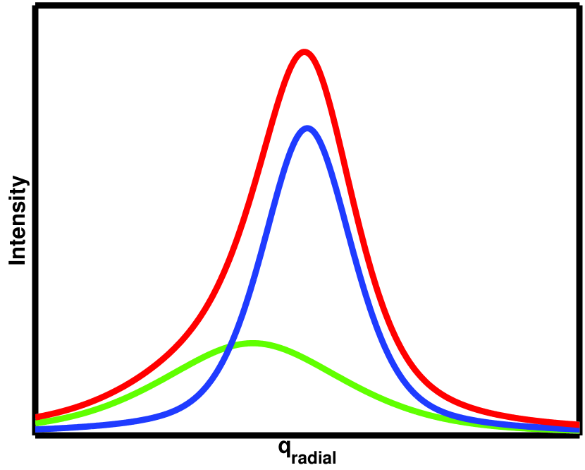
Figure 2.2: Left) Illustration of the composite model of a deformed cell forming metal under a tensile load. $\sigma$ is the applied stress , $\Delta\sigma_{w}$ and $\Delta\sigma_{c}$ are the forwards and backwards stresses in the walls and cell interiors respectively. $\bm{q}_{\text{axial}}$ and $\bm{q}_{\text{side}}$ indicate the direction of the scattering vector for the axial and radial cases respectively. Right) Illustration of an asymmetric peak in the axial case (red line), and the decomposition into a part from the cell interior (blue line) and a part from the walls (green line).

2.4 Experimental investigation of diffraction

Three basic methods exist for investigating the diffraction signal from crystalline samples: The rotation method, the Laue method, and the powder method.

The first two of these methods has classically been used on single crystals, and the latter on powder samples. However, with the use of modern synchrotron radiation it is possible to investigate single grains in polycrystalline samples (see section 2.5.1 and 2.5.2). The Laue method uses a polychromatic X-ray beam, whereas a monochromatic beam is used for the other two methods.

The monochromatic techniques will be discussed in the following, as they are the basis for the developed technique. Reciprocal space mapping will furthermore be discussed.

2.4.1 The rotation method

A typical setup for investigating the diffraction signal by use of the rotation method in the transmission mode is shown in figure 2.3. The sample is illuminated by a monochromatic beam and the diffracted beam is recorded on an area detector. Lattice planes that happen to fulfill the diffraction condition will give rise to a diffraction spot on the detector, and by rotating the sample, different reflections can be brought into the scattering condition.

In the rotation method, data is obtained by rotating the sample with constant angular velocity over some angular range, $\Delta\phi$, around a fixed axis (on the figure the $\bm{y}$-axis), while exposing. There are two reasons for this. Firstly, the reflections are very close to delta shaped if the sample is a perfect crystal, hence it is very hard to align the sample precisely at the scattering condition. Secondly, it will lead to a integration over the full intensity in a reflection if it has some width in reciprocal space.

Such a single exposure integrates over some part of reciprocal space. To sample a larger part of reciprocal space many exposures are taken at adjacent angular intervals.

Figure 2.3: Typical setup for the rotation method, using a transmission geometry and an area detector. Data is obtained by rotation the sample over some angle around the $\bm{y}$-axis while exposing. The scattering angle, $2\theta$, azimuthal angle, $\eta$, and rotation angle $\phi$ are defined.

The total integrated diffracted intensity for one reflection $E_{hkl}$, is given by [warren1969]:

$$E_{\text{crystal}}=\frac{I_{0}}{\dot{\omega}}\left(\frac{e^{4}}{m_{e}^{2}c^{4}}\right)\frac{\lambda^{3}V_{\text{crystal}}\left|F_{hkl}\right|^{2}}{v_{a}^{2}}P(\theta_{hkl},\eta)\frac{1}{\sin(2\theta_{hkl})|\sin{\eta}|}$$ (2.27)

where $\dot{\omega}$ is the angular velocity used for the measurement, $V_{\text{crystal}}$ is the volume of the scattering crystal, $I_{0}$ is the input intensity (energy per time per area), $P(\theta_{hkl},\eta)$ is the polarization factor which depends on the polarization of the X-ray beam, $\eta$ is the azimuthal angle for the reflection, $\theta_{hkl}$ is the scattering angle for the given reflection family, $F_{hkl}$ is the structure factor for the given reflection family, $v_{a}$ is the volume of the unit cell and $e,m_{e}$ and $c$ are fundamental constants: charge of the electron, mass of the electron and speed of light, respectively. The last term in the equation is normally called the Lorentz factor, and depends on the details of the setup.

What is most interesting for the present study is that the intensity is linear in the diffracting volume.

2.4.2 The powder method

A powder sample consists of a large number of small (with respect to the beam size) crystallites.

The crystallites have some distribution of orientations (known as the texture of the powder). Generally a large number of crystallites will fulfill the scattering condition when the sample is illuminated at any orientation. Data is normally obtained with a stationary sample, using a monochromatic beam. The signal on the detector consists of what is known as Debye-Scherrer rings.

The integrated diffracted intensity per angular unit in one Debye-Scherrer ring from a powder with random orientation of the crystallites is given as:

$$E_{\text{powder}}=I_{0}\left(\frac{e^{4}}{m_{e}^{2}c^{4}}\right)\frac{\lambda^{3}V_{\text{powder}}m\left|F_{hkl}\right|^{2}}{v_{a}^{2}}P(\theta_{hkl})\frac{1}{4\sin(\theta_{hkl})}\frac{\Delta t}{360\mathrm{\SIUnitSymbolDegree}}$$ (2.28)

where $V_{\text{powder}}$ is the volume of the powder that is illuminated, $\Delta t$ is exposure time, $m$ is multiplicity of the reflection family, and other symbols have the same meaning as in equation 2.27. Equation 2.28 is derived under the assumption of an unpolarized beam (as from a conventional X-ray source), which simplifies the calculation. However, in the case of synchrotron radiation the beam is almost linear polarized in the horizontal plane, which means that equation 2.28 in the general case has to be modified. As the general result is not needed for the present studies further discussion of this will be postponed to section 3.6.5.

2.4.3 Investigation of intensity distributions

In section 2.3 it was discussed what can be learned from the shape of the individual diffraction peaks, the reflections. The reflections will in general be a three dimensional, intensity distribution in reciprocal space, close to the corresponding theoretical reciprocal lattice point.

3D intensity distributions have normally been investigated in a number of ways, such as: line profile analysis, rocking curve analysis, 2D reciprocal space mapping, and 3D reciprocal space mapping. Beside the 3D mapping, these techniques represent a projection onto either a line or plane of the full intensity distribution.

Figure 2.4: General schematic of a classic point detector-based diffraction setup. $\bm{k}_{0}$ and $\bm{k}$ are the incoming and outgoing wave vectors respectively, $\theta$ is the scattering angle and $\Delta\omega$ the misalignment in the scattering plane between the ideal lattice plane normal and the scattering vector.

The schematic layout of the classic experimental setups for these types of measurements are generally much alike Figure 2.4 shown a schematic of such a setup based on a point detector. In the following some of the different applications will be discussed.

Line profiles and rocking curves

Classic integrated radial line profiles are obtained by integrating over the azimuthal directions, and investigating the intensity as a function of the length of the scattering vector (keeping the angle between the sample surface and scattering vector constant). Such curves are normally obtained by $\theta$,$2\theta$ scans, where the sample and detector are rotated in steps of $\Delta\theta$ and $2\Delta\theta$ respectively. It can be seen from figure 2.4 that such a scan will keep the direction of the scattering vector, $\bm{q}$, constant with respect to the sample surface while changing the length. The integration over the azimuthal direction out of the scattering plane is normally obtained by having a rather large beam divergence in this direction. The in-plan azimuthal broadening is normally integrated over by rotating the sample over an angle, $\Delta\omega$, for each $\theta,2\theta$ point.

The intensity distribution in the azimuthal direction can be investigated by what are known as rocking curves. The sample is here rotated with a constant speed in small steps around an axis perpendicular to the scattering vector (as e.g. represented by the angle $\Delta\omega$ on figure 2.4) while recording the intensity. An integration over the radial and the other azimuthal direction can be obtained by suitable combinations of beam divergence and energy spread in the X-ray beam used.

Reciprocal space maps

The two above techniques can easily be generalized to 2D and 3D dimensional reciprocal space maps (for a review of such techniques see e.g. [Fewster1997]).

Most common is a projection onto the plane of the radial direction and the in-plane azimuthal direction. Such a map can be obtained by gathering radial line profiles for different angles between the sample and the scattering vector. This corresponds to $\theta$,$2\theta$ scans with different $\Delta\omega$ in figure 2.4. This requires a beam with a narrow energy spread, and a low divergence in the scattering plane (an example of a diffractometer enabling such maps can be found in [Fewster1989]).

By limiting the divergence in both the in plane and out of plan directions, it is possible to obtain full 3D reciprocal space maps by introducing a second rotation axis for the sample (e.g. [Fewster1995]). The problem with such techniques are that they are point-by-point in a 3D space, hence acquisition time rises quickly with the resolution obtained. Furthermore the resolution tends to be different in the three directions.

2.5 Recent developments

The Laue and rotation methods have normally been used on single crystals. However, with the availability of synchrotron radiation and X-ray optics they have been generalized to multi-grain samples.

These generalizations are based on the fact that the individual grains in a multi-grain sample can be investigated using the classic methods if the beam size, sample properties (such as thickness and grain size) and other experimental parameters are matched.

In the following three methods will be discussed as they have special relevance for the problems investigated here.

It should also be mentioned that a large number of experiments which normally were performed on home sources can now be performed in improved versions using synchrotron radiation (a few examples are [Chang1995; Biermann1997; Murphy2001; Schafler2005]). These improvements are normally better time and spatial resolution due to the much larger flux.

2.5.1 3DXRD microscopy

The 3D X-ray diffraction (3DXRD) method is a monochromatic synchrotron-based technique, for comprehensive characterization of the structural properties of individual grains deeply embedded in polycrystalline samples. A detailed description of the technique is found in the book by H. F. Poulsen [poulsen04:bog], and a detailed description of the geometry is found in [Lauridsen2001].

The method is based on the rotation method as described in section 2.4.1, but generally applied to polycrystalline samples. The sample is illuminated by a monochromatic beam, and the diffracted signal (in transmission mode) is recorded by use of an area detector behind the sample (as on figure 2.3). Overlap between reflections from different grains are avoided by matching the size of the angular rotations and beam size, with respect to the structural characteristics of the sample (grain size, sample thickness, mosaic spread and texture). Each detector image obtained includes diffraction spots from many grains, but each spot is generally only associated with one grain.

The dedicated 3DXRD setup at the ID-11 beam-line at the European Synchrotron Radiation Facility (ESRF, Grenoble) can be used in different modes:

Spatial information

on the shape of individual grains can be prioritized for e.g. mapping of grain shapes during grain growth [Poulsen2001; Schmidt2004].

Time resolution

can be prioritized for e.g. in-situ studies of grain growth
[Nielsen2003].

Angular resolution

can be prioritized for e.g. analysis of grain rotation during deformation [Margulies2001].

Many grains in a polycrystalline sample can be investigated simultaneously due to the topographic approach to diffraction. The technique furthermore has the advantage that only one (angular) degree of freedom has to be scanned during data acquisition, in contrast to spatial scanning techniques.

The variant which is of relevance for the present study is what might be termed “far-field 3DXRD” where the detector is positioned so far from the sample that multiple full reflection families (Debye-Scherrer rings) are investigated. The orientation of the individual grains can be determined from such data.

A fundamental part of the technique is the GRAINDEX program, by which it is possible to assign the individual diffraction spots obtained from a polycrystalline sample to individual grains.

The individual reflections are first assigned to $hkl$ families, and then by means of an algorithm known as “the grain digger” assigned to grains [Lauridsen2001]. The output of the algorithm is a list of grains. For each grain the algorithm gives the orientation matrix, associated reflections, and statistical information on how confident the finding of the grain is.

The most important statistical information are the uniqueness and completeness of the grain. The completeness measure how many of the theoretically accessible reflections have been found for the given grain. The uniqueness measure how many of the reflections assigned to a given grain that are also assigned to a different grain.

2.5.2 The 3D crystal microscope

The 3D crystal microscope is a white-beam (Laue) synchrotron-based technique. This method is, as opposed to the 3DXRD method, a point-by-point measuring method using a micrometer sized beam and what is known as differential-aperture X-ray microscopy [Larson2002].

The dedicated setup at APS is described in details in [Ice2005], and a recent review of the technique and results are given in [Ice2006].

By use of X-ray optics the white-beam is focused to a sub micrometer spot ($0.5\times 0.5\mathrm{\SIUnitSymbolMicro}\mathrm{m}$). By scanning such a beam over the sample the structure can be probed in a 2D grid, but still probing all the material along the beam. The resolution in the depth is obtained by scanning an absorbing wire through the diffracted beam. Figure 2.5 illustrates the basic idea of the technique. By triangulation it is possible to reconstruct the Laue pattern from individual 3D voxels in the sample (the resolution in the direction along the beam is $0.5$ – $0.7\mathrm{\SIUnitSymbolMicro}\mathrm{m}$).

Local phase, crystal orientation and distortion of the unit cell can among other material parameters be gathered from the reconstructed Laue patterns. By modelling and simulation information can furthermore be obtained on the dislocation distribution.

The major limitation to the technique is that the point-by-point data acquisition is very time consuming, and it can also be debated to what extent true bulk measurements may be performed as the energy is rather low (results presented in [Ice2006] go to a depth of $30\mathrm{\SIUnitSymbolMicro}\mathrm{m}$ in a Cu sample, but it is not explicitly stated that this is the depth limit).

The technique has recently been extended to what is termed “scanning monochromatic differential-aperture X-ray microscopy” [Levine2006]. The technique is specialized toward spatial measurements of elastic strains. It is, as indicated, a monochromatic technique. A tunable monochromatic beam (X-ray energy $\approx 14\mathrm{k}\mathrm{eV}$) is used instead of a white beam, hence directly giving the lattice spacing in the illuminated sample part. The strain resolution is reported to be $\Delta q/q=1-2\cdot 10^{-4}$.

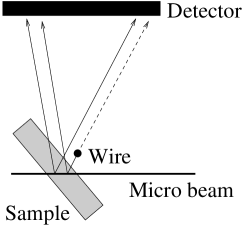
Figure 2.5: Schematic of the 3D X-ray crystal microscope. The wire is moved in steps parallel to the sample to obtain spatial information along the beam.

2.5.3 3DXRD peak shape analysis

The 3DXRD microscopy method has been generalized such that reciprocal space maps can be obtained for the individual reflections from deeply-embedded individual grains in a polycrystalline sample (a techniques which here will be termed “3DXRD peak shape analysis”). The technique was introduced in [pantleon04].

A specialized setup was developed at the 1-ID beam line at APS. By using of a narrow bandwidth monochromator and positioning the detector far from the sample a high resolution image was obtained in reciprocal space. By integrating the stress rig into the setup it is possible to do in-situ measurements.

The detector used was a 2D CCD detector, and by acquiring data while rotating the sample over equidistant intervals (rocking) a 3D reciprocal space map could be generated of a reflection. As is general for the 3DXRD method the properties of the sample and beam were matched, so that the reflections from the individual grains did not overlap.

Multiple reflections from the same grain can be found by use of the GRAINDEX program. The data acquired for this were taken using a large area CCD detector close to the sample (in the “far field 3DXRD” geometry).

In [pantleon04] measurements on 20 reflections from the same grain were characterized at tensile strains of $0\%$, $1\%$, $2.5\%$ and $4.5\%$. The radial peak profiles (integrating in the azimuthal directions) show asymmetries, which in some cases are in line with what should be expected from the composite model (see page 2.3.1), but in other cases derivate from the expected. This is rationalized in term of an anisotropy in the dislocation structure. The azimuthal profiles were used for obtaining the orientation distribution function for the grain [Poulsen2005]. The method was further used for evaluating the effect of grain interactions during plastic deformation [lienert04:cu].

Compared to traditional line broadening studies the technique has multiple advantages. The measurements are specific to the individual grains, multiple reflections can easily be investigated for the same grains and the data obtained are full 3D reciprocal space maps of the reflections. Compared to traditional reciprocal space mapping, the technique has the advantage that only one angular degree of freedom has to be scanned, due to the use of a 2D detector.

One of the ideas behind developing the setup was to gather in situ information on development of deformation structures. However, the interpretation of the reciprocal space maps still required heavy use of models.

Just as the 3DXRD method avoids the averaging over multiple grains, it turned out that by enhancing the resolution in reciprocal space, this method could be turned into a direct probe for the individual subgrains. This lead to the development of the “High Angular Resolution 3DXRD” method as described in the major part of this thesis.

Chapter 3 High Angular Resolution 3DXRD

The novel technique “High Angular Resolution 3DXRD” is presented in this chapter.

The technique will be briefly described in section 3.1 including examples of the raw data and a presentation of the interpretation. The experimental setup is described in section 3.2 followed by details on data taking and coordinate systems in section 3.3 and 3.4. The instrumental resolution is discussed theoretically and experimentally in section 3.5. The different methods for analyzing the data are presented in section 3.6. The reproducibility of the results is discussed in section 3.7 followed by detailed argumentation for the interpretation of the data in section 3.8. High Angular Resolution 3DXRD is finally compared to other relevant techniques in section 3.9.

3.1 Overview

This section gives an overview of the technique developed, the raw data obtained, the interpretation of the measurements, and a discussion of why a new technique is needed. The choice of samples is also discussed. This is a brief introduction and all issues will be discussed in detail in the following sections.

3.1.1 The technique

The aim of the technique developed is, as described in the introduction, to obtain high resolution reciprocal space maps of the broadened reflections from a deformed metal.

The experiments were performed at the 1-ID beam line at the Advanced Photon Source (APS), where a unique combination of X-ray optics, detectors and mechanical setup enables 3D reciprocal space mapping with a high resolution, and a reasonable acquisition time.

The method is developed on the basis of the “3DXRD peak shape analysis” technique [pantleon04] described in the previous section (section 2.5.3). The present setup allows for substantially higher resolution in full 3D in reciprocal space, whereas the old setup was focused on obtaining low resolution peak shapes for a more traditional model-based analysis.

The main difference between the setups, is that the present setup includes X-ray optics for focusing the beam onto a small area. This is needed if high resolution maps are to be obtained in a feasible time. Furthermore the energy is different, and a different set of monochromators were introduced.

The basic setup is shown in figure 3.1. The sample is illuminated by a monochromatic X-ray beam, and the diffracted signal recorded on one of the two available detectors. The sample is mounted in an Euler cradle allowing for rotation of the sample. This cradle is also used for rotation during exposure.

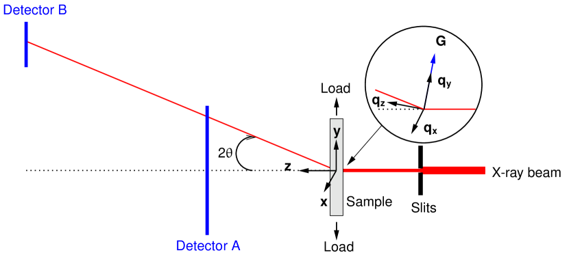
Figure 3.1: Sketch of the setup, showing the two detectors, sample and slits. The laboratory and reciprocal space coordinate systems are defined. From science.

Detector A is used for gathering “far-field 3DXRD” data (see section 2.5.1). Such data are used either for finding the full orientation of diffracting grains by use of the GRAINDEX program, or for a manual search for interesting reflections (see section 3.3).

Detector B is used for obtaining the high resolution 3D reciprocal space maps. This is done by rotating the sample around the $\bm{x}$-axis in small consecutive intervals while obtaining data (the rocking method as described in section 2.4.3).

Figure 3.2 shows 9 such consecutive images as obtained on the detector. The sample is a Cu sample deformed to $2\%$ in tension, and the investigated reflection is a 400 reflection. A 3D reciprocal space map is constructed by stacking such 2D images.

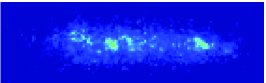
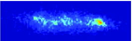
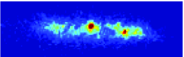
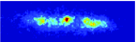
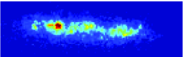
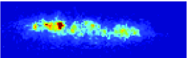
Figure 3.2: Raw data. Each figure represents the intensity as recorded on the detector while rocking $0.007\mathrm{\SIUnitSymbolDegree}$ around the $\bm{x}$-axis. Each image covers a range of $0.6\mathrm{\SIUnitSymbolDegree}$ horizontally (in $\eta$) and $0.05\mathrm{\SIUnitSymbolDegree}$ vertically (in $2\theta$). Read from left to right, top to bottom, the figures show consecutive intervals. The reciprocal 3D space map is generated by stacking such images. From acta.

3D reciprocal space mapping is, as mentioned in section 2.4.3, no new technique (see e.g. [Fewster1997]). The advantage of the present setup is that due to the 2D detector a full 2D part of the reciprocal space is mapped per image obtained, in contrast to traditional point-by-point acquisition. The present method further has the advantage that the resolution is about equal in all three reciprocal space directions, and that the resolution can be changed by changing the rocking interval size and sample-to-detector distance.

3.1.2 Interpretation of data

From figure 3.2 it is observed that the broadened reflection comprise a cloud of enhanced intensity upon which bright peaks are superimposed. The observable peaks are clearly separated in all three reciprocal space directions.

Our interpretation of these structures, in the reciprocal space intensity distribution, is that the individual peaks arise from individual dislocation free subgrains in the dislocation structure, and that the cloud stems from the dislocation-filled walls (the arguments for this interpretation are given in section 3.8).

The radial position of the peaks are directly related to the mean strain in the scattering region, the width of the peak to the strain distribution within the scattering region, and the integrated intensity to the volume of the scattering region.

The techniques hence allows for a direct, model free, non-destructive investigation of these properties, (mean strain, internal strain distribution and volume), of the individual subgrains. The properties can be investigated in-situ from dislocation structures deeply imbedded in individual bulk grains in a polycrystalline sample.

3.1.3 Samples

The technique described in this chapter can naturally be used for obtaining data on single crystals but multiple issues (both experimentally and scientific) might suggest the investigation of polycrystalline samples.

The use of polycrystalline samples has the advantage that the grain size will limit the investigated volume in the direction of the beam. If this volume is to large, the possibility of overlap between the peaks from the individual subgrains becomes large, and it is impossible to separate them. In the case of single crystal samples the thickness would therefore have to be small, or the volume would have to be restricted by other means (a possibility is the use of a conical slit [Nielsen2000] or wire scanning techniques [Larson2002]). The use of polycrystalline samples has the further advantage that multiple grains with different orientations can be investigated under the exact same macroscopic stress/strain conditions.

The chosen material for most of the experiments was, as mentioned in the introduction, polycrystalline copper. The material used is $99.99\%$ pure OFHC copper. The precise details of the samples vary between the individual experiments (see table 4.1). Generally the material was cold rolled to a reduction of $80\%$ to a final thickens of $300\mathrm{\SIUnitSymbolMicro}\mathrm{m}$ and then fully recrystallized by annealing. The material was characterized by electron backscattering diffractions (EBSD), and the mean grain size was found to be $\approx 30$ – $36\mathrm{\SIUnitSymbolMicro}\mathrm{m}$, resulting in about ten grains across the thickness of the sample.

3.2 The setup at 1-ID (APS)

The setup is illustrated on four figures: figure 3.1 which gives an overview of detectors, sample and stress rig, figure 3.3 which illustrates the X-ray optics, figure 3.5 (page 3.5) showing a photograph of the main part of the setup, and figure 3.7 (page 3.7) which focuses on scattering geometry for reciprocal space mapping.

The following main components will be described in detail below:

• X-ray optics providing a focused beam with low beam divergence and low relative energy spread. Included is also a slit system defining the final beam size and beam position with respect to the sample.

• A custom made stress rig, allowing for in-situ deformation.

• Translations and a Huber Euler cradle, allowing for positioning and rotating the sample.

• An area detector close to the sample for gaining “far-field 3DXRD” data for an overview of available reflections, also used for obtaining data for analyzing with the GRAINDEX program. This detector is mounted on a horizontal translation stage which allows it to be translated out of the diffracted beam.

• An area detector placed far from the sample, mounted on a vertical translation stage, used for obtaining the high resolution reciprocal space maps.

3.2.1 Optics and beam monitoring

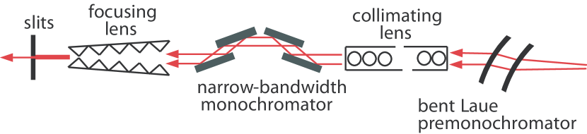
Figure 3.3: Sketch of the X-ray optics setup. From science, Supporting Online Material.

An overview of the optics developed by the APS sector-1 collaborators is provided in figure 3.3. The optics consists of (see [ science] and [Shastri2004]): a pre-monochromator (two bent Laue crystals) [Shastri2002], a collimating refractive lens, a narrow-bandwidth monochromator (two channel cut crystals) and a set of saw tooth lenses for focusing [Cederstrom2002].

By this combination of optics the beam obtained a unique combination of properties: High energy ($52\mathrm{k}\mathrm{eV}$), low vertical divergence ($17\mathrm{\SIUnitSymbolMicro}\rad$), small relative energy spread $\frac{\Delta E}{E}=7\cdot 10^{-5}$, and high flux [ science]. The horizontal beam divergence is given by the source size and distance from this to the sample as no focusing exists in this directions [ulli], and is $\approx 13\mathrm{\SIUnitSymbolMicro}\rad$.

The low divergence and low energy spread allows for a high resolution of the reciprocal space mappings, and the high flux (due to the focussing) for a reasonable acquisition time.

The final beam size impinging on the sample is defined by a set of slits positioned close to the sample ($\approx 30\mathrm{c}\mathrm{m}$). The intensity of the beam impinging on the sample is monitored by an ion chamber positioned behind (downstream of) the slits (seen on figure 3.5).

The position of the focal point of the focusing optics can be varied. The optimal flux would be obtained by focusing directly on the sample position, but as this in practice is difficult (since no beam monitor exists at this position) the focus point is either positioned at the slits before the sample, or on a high resolution detector which is positioned $\approx 1\mathrm{m}$ behind the sample. In the later case, the result is a vertical focal size of the beam at the sample position of $\approx 25\mathrm{\SIUnitSymbolMicro}\mathrm{m}$. The total aperture of the focusing lenses is about $400\mathrm{\SIUnitSymbolMicro}\mathrm{m}$ and the integrated transmission $\approx 80\%$ [ulli]. Taking into account the non-box-shape of the beam, the gain in total intensity is approximately a factor of $10$. Using the slits the beam can be reduced to the vertical size needed.

Measurement of the beam profile

The beam at the sample position can be characterized by scanning a diffracting object through the beam and recording the scattered intensity. An example of a beam profile determined in this way is shown in figure 3.4. The profile is found by scanning a LaB₆ grain through the beam, the precise size of the grain is unknown, but the mean size of the grains is $\approx 2\mathrm{\SIUnitSymbolMicro}\mathrm{m}$ [lab6], hence it is much smaller than the width of the beam. The slit size was nominal $\approx 20\mathrm{\SIUnitSymbolMicro}\mathrm{m}\times 20\mathrm{\SIUnitSymbolMicro}\mathrm{m}$ (approximately as the experimental run from which the data shown in figure 3.4 originate, suffered from problems with the motor drive of the slit blades). It is seen that the beam is box shaped in the $x$-direction, and bell shaped in the $y$-direction; as expected.

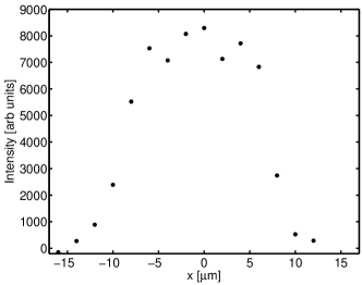
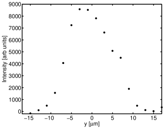
Figure 3.4: Beam profile at the sample position in the horizontal ($x$) and vertical ($y$) directions. The profiles are acquired by scanning a micrometer sized LaB₆ grain through the beam and recording the scattered intensity.

Beam stability

The slits are fixed with respect to the diffractometer. This has the consequence that if the beam moves in the vertical direction the illuminated part of the sample remains the same, but the total intensity and the intensity profile of the beam at the sample position might change. Due to the long ($\approx 21\mathrm{m}$) distance from the optics to the sample, even very small changes in angles will give detectable changes in vertical beam position at the slits, resulting in a change of the beam profile at the sample. Such instabilities have been a problem throughout this study.

The changes in absolute intensity can easily be corrected for, by recording the integrated incoming intensity during data acquisition by the ion chamber before the sample. More challenging is the change in beam profile, as this will lead to changes in relative intensities arising from different parts of the sample. A solution might be a feedback system on the optics, reducing the drift of the beam position.

3.2.2 Stress rig

The stress rig (shown in figure 3.5) is custom built to fit in the Euler cradle, so that in-situ experiments can be performed. The rig is displacement-controlled, and the deformation speed can be chosen in the range from very slow (experiments have been done as slow as $\approx 4\cdot 10^{-5}\mathrm{m}\mathrm{m}\mathrm{/}\mathrm{s}$ ) to rather fast (fastest experiment was done at $\approx 0.6\mathrm{m}\mathrm{m}\mathrm{/}\mathrm{s}$).

The load on the sample is monitored by a load cell mounted below the sample. The load cell is read out by a control box, and readings are recorded by a logging system. The tensile stress on the sample is proportional to the measured load, as the gauge area of the sample is assumed to be constant.

The strain is monitored by a strain gauge glued directly onto the gauge area of the sample. The strain gauge is read out using a Wheatstone bridge, and recorded by a logging system.

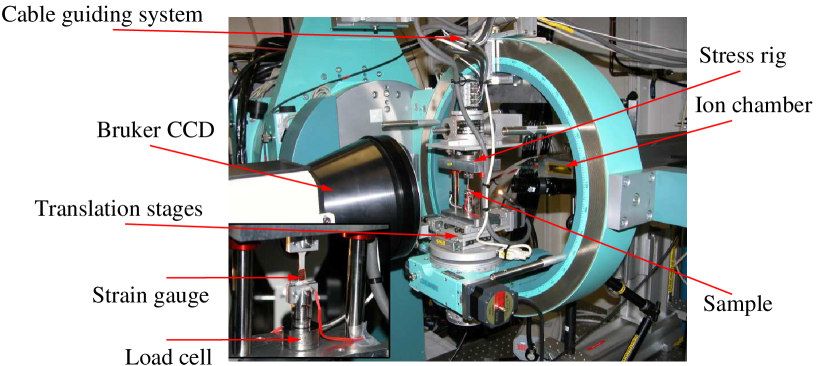
Figure 3.5: Photograph of the main optical table showing: The stress rig mounted on the Huber Euler cradle, the Bruker CCD detector and visible through the Euler cradle the ion chamber. The insert shows a sample (this is an Al sample of different size than the Cu samples normally used) mounted in the stress rig. A strain gauge is visible on the sample. The load cell is the round device below the sample.

3.2.3 Euler cradle

The Huber Euler cradle allows for rotations around three axes. A 3-axis translation is mounted on the inner rotation allowing for translation of the stress rig/sample.

The order of the rotations is such that (see figure 3.7 on page 3.7 for a definition of the rotations) $\phi$ is the inner rotation, $\chi$ the middle rotation and $\omega$ is the outer rotation.

On figure 3.5 the cradle is shown with the stress rig mounted. A cable guiding system is seen at the top of the image; this allows for free rotation of the stress rig, without human intervention.

Before measurements, the center of rotation of the cradle is made to coincide with the center of the beam. The centering is based on scanning a pin through the beam, and the geometry of the setup.

However, for mechanical reasons the Euler cradle, with the mounted stress rig, does not have a totally well-defined center of rotation (a problem known as the sphere of confusion). This has the unfortunate consequence, that if a grain is centered in the beam at one $\phi$, $\omega$, $\chi$ setting, it might be off center at another angular position. The sphere of confusion can be measured in different ways, and corrections applied, however for most of the experiments presented the problem is minor, as the sample normally is only rotated a few degrees in the critical angles.

The $\omega$ rotation (which always is around the $\bm{x}$-direction), is used for the rocking procedure for gathering the high resolution 3D maps. An investigation showed that the drive could produce steps as small as $0.0005\mathrm{\SIUnitSymbolDegree}$, or better.

3.2.4 Detectors

The setup comprises two detectors (as shown on figure 3.1). Detector A is used for obtaining low angular resolution data comprising many reflections from many grains (far field 3DXRD data). Detector B is the main detector used for obtaining reciprocal space maps. Detector A is moved out of the diffracted beam when data are to be acquired using detector B.

Detector A

Detector A is a Bruker SMART 6500 CCD area detector. It is positioned $\approx 0.3\mathrm{m}$ from the sample. The exact distance varied from experiment to experiment, and was calibrated together with the position of the direct beam by a measurement on a known powder sample. The detector is close enough to the sample to allow the full 400 reflection family to be recorded when using copper samples and an X-ray energy of $52\mathrm{k}\mathrm{eV}$. The detector has a pixel size of $161\mathrm{\SIUnitSymbolMicro}\mathrm{m}\times 161\mathrm{\SIUnitSymbolMicro}\mathrm{m}$ when used in $1024\times 1024$ pixel mode [bruker].

Detector B

Detector B is a MarCCD 165 area detector, positioned at a horizontal distance of $\approx 3.9\mathrm{m}$ from the sample. The exact position varied between the experiments and was found by calibration measurements. The detector is mounted on a vertical translation stage allowing for mapping different $hkl$’s.

The detector has been used in either $2048\times 2048$ pixel or $1024\times 1024$ pixel mode, the latter used for reduced readout time. The pixel size is $80.5\mathrm{\SIUnitSymbolMicro}\mathrm{m}\times 80.5\mathrm{\SIUnitSymbolMicro}\mathrm{m}$ and $161\mathrm{\SIUnitSymbolMicro}\mathrm{m}\times 161\mathrm{\SIUnitSymbolMicro}\mathrm{m}$ respectively. The full width at half maximum of the point spread function is $100\mathrm{\SIUnitSymbolMicro}\mathrm{m}$ [marccd].

3.3 Selecting grains and reflections

Before data can be obtained a reflection from an interesting grain (in the case of polycrystalline samples) has to be selected and centered on the detector.

The grain is typical centered within the X-ray beam by spatial scanning of the grain with respect to the beam, and recording the diffracted signal.

Two strategies for selecting reflections/grains have been employed in this study, and will be described below. The first strategy is based on a choice of reflection without full information on the orientation of the scattering grain. The second strategy is based on full information about the grain orientation as obtained from the 3DXRD technique (section 2.5.1).

3.3.1 Reflection-based selection of a grain

An overview over available reflections can be obtained by using detector A (close to the sample), and then simply scanning the orientation and position of the sample. By means of this a suitable reflection can be identified, typically based on a criterion on the angular separation between the chosen reflection and neighboring reflections.

Based on one such reflection the corresponding grain can easily be centered in the beam in the $\bm{x}$ and $\bm{y}$ directions. In principle it is furthermore possible to clarify if the grain is within bulk or close to the surface. Several trigonometry-based methods have been devised but due to experimental uncertainties (mainly the sphere of confusion problem discussed in section 3.2.3) no perfect and stable method exists (see section 3.3.3).

Based on one reflection it is possible to calculate the angle between the tensile axis and the normal vector corresponding to the scattering lattice planes. This leaves one rotational degree of freedom for the full orientation of the tensile axis with respect to the crystallographic coordinate system of the grain. In figure 3.6 the possible orientations of the tensile axis, as represented in an inverse pole figure, are shown for multiple cases of 100 reflections with a fixed angle between the tensile axis and lattice normal. It is seen that in the case where the angle between the tensile axis and the $\{100\}$ lattice plane normal is $0\mathrm{\SIUnitSymbolDegree}$ full information about the orientation of the tensile axis is obtained, whereas in the case of $90\mathrm{\SIUnitSymbolDegree}$ the orientation can be anywhere between $\langle 100\rangle$ and $\langle 110\rangle$. The orientation of the tensile axis is known to control the morphology of the microstructure [huang97] (see section 1.1.2).

This method for finding relevant reflections has been widely used in the present study as most investigations have been made on grains with the tensile axis close to a $\langle 100\rangle$ crystallographic direction.

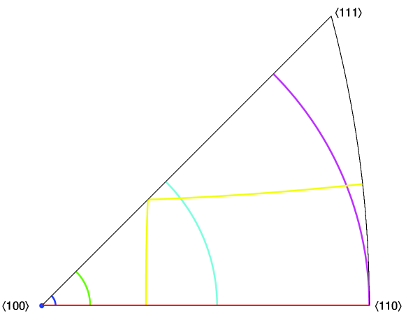
Figure 3.6: Inverse pole figure shoving possible orientations of the tensitle axis in the crystallographic-coordinate-system, for known angles between the tensile axis and the $\left\{100\right\}$ lattice plane normal. The angles shown are $0\mathrm{\SIUnitSymbolDegree}$ (*), $2\mathrm{\SIUnitSymbolDegree}$ (blue line), $7\mathrm{\SIUnitSymbolDegree}$ (green line), $25\mathrm{\SIUnitSymbolDegree}$ (cyan line), $45\mathrm{\SIUnitSymbolDegree}$ (magenta line), $75\mathrm{\SIUnitSymbolDegree}$ (yellow line), and $90\mathrm{\SIUnitSymbolDegree}$ (red line).

3.3.2 Grain-based selection of reflections

Alternatively to working directly on reflections, a list of grains from the GRAINDEX program (as described in section 2.5.1) can be utilized.

By working with the list of grains, and the list of reflections found, it is possible to find grains and corresponding reflections which have certain properties. Generally the search is for grains of a certain orientation having interesting reflections, which are angularly separated from reflections of other grains. A number of MATLAB routines have been developed for this.

When the full orientation is known it is furthermore possible to investigate multiple reflections from the same grain. This is very important as some existing theoretical predictions (e.g. [Mughrabi1983]) and experimental results on single crystals (e.g. [Ungar1984]) show that differences exists between different reflections from the same crystal (see section 2.3.1).

3.3.3 Ensuring that a grain is in the bulk

GRAINDEX-based methods

The information from the GRAINDEX program can be used in two ways to find individual grains which are in the bulk of the sample.

The first method is based on the observation that the completeness parameter associated with each grain found (see section 2.5.1) is unlikely to be high for a grain not in the bulk of the sample. This is true under the following conditions:

• The sample is positioned such that the center of the sample is at the center of rotation of the Euler cradle.

• The vertical beam size used is much smaller than the thickness of the sample.

• The grains are substantially smaller then the thickens of the sample.

• The dataset obtained for the GRAINDEX analysis covers a substantial angular range.

A grain not in the bulk of the sample will rotate out of the beam at some point during the data acquisition, if these requirements are met. The consequence is that a number of expected reflection will be missing, and GRAINDEX will therefore return a low completeness.

Secondly, the knowledge of the full orientation of the grain, allows for selecting multiple reflections from the same grain, which are separated by some rotation around the $\bm{y}$-axis. The full position in the $(\bm{x},\bm{z})$ plane can be found by scanning the grain through the beam at two such different orientations. It can therefore be directly determined if the grain is in the bulk of the sample.

Single reflection-based methods

If only one reflection from a grain is known it is still possible to find different angular settings of the Euler cradle which gives access to the reflection. It is therefore possible by triangulation to find the full spatial position of the grain, and hence to determine if it is in the bulk.

A simple example is that a grain rotated by an angle of $2\theta$ around an axis perpendicular to the scattering plane will bring “minus” the scattering vector into scattering condition.

The problem of such methods is that the sphere of confusion makes it difficult to determine if the grain is in the bulk of the sample.

3.4 Reciprocal space mapping

The general considerations about obtaining 3D reciprocal space maps will be presented in this section and a useful reciprocal space coordinate system will be defined.

Figure 3.7 is general for this section. It defines the real space coordinate system, available rotations angles and illustrates the reciprocal space coordinate system.

Figure 3.7: Sketch of the experimental setup. Defining the laboratory coordinate system $\bm{x}$, $\bm{y}$ and $\bm{z}$, available rotations of the Eulerian cradle $\phi$, $\chi$ and $\omega$ (with $\phi$ the inner rotation and $\omega$ the outer), angles $2\theta$ and $\eta$, and reciprocal space coordinate system $\bm{q}_{x}$, $\bm{q}_{y}$ and $\bm{q}_{z}$. In the indication of the angle between the $\bm{q_{z}}$-axis and the horizontal plane, $\theta_{0}$ is the scattering angle of the undeformed sample, and $\omega$ is to be read as the present value of this rotation with respect to vertical. $L$ is the horizontal distance between the detector and the point of rotation of the Eulerian cradle. The tensile axis is along the $\bm{y}$-direction for $\omega=0$, and $\chi=0$. From [ acta].

3.4.1 Data collection

As shown on figure 3.7, the sample is placed in a 3-axis rotation stage and illuminated by a monochromatic X-ray beam. The diffracted signal (in transmission mode) is recorded on an area detector positioned on a vertical translation stage behind the sample.

Before data can be obtained from a desired reflection, from a specific grain, the sample is rotated, and the detector translated, such that the reflection gives rise to a diffraction signal on the detector. That is, the sample is rotated such that the diffraction condition, for the relevant reflection, is fulfilled with the scattering vector close to the $(\bm{y},\bm{z}$)-plane, and the detector translated to the relevant height for the scattering angle of the reflection.

Obtaining reciprocal space maps

Data are (as described in section 3.1.1) obtained by rocking. By this a 3D part of reciprocal space is mapped onto the detector, by integrating out one dimension. In the present setup the $\omega$ rotation is used for the rocking (as it is approximately perpendicular to the scattering planes for the investigated $\bm{q}$- vectors). The rocking interval is termed $\Delta\omega$ and one image on the detector is termed an $\omega$-slice. By acquiring and stacking adjacent $\omega$-slices a 3D map of a part of the reciprocal space is obtained. Each point in this dataset represents the integrated intensity of a voxel in reciprocal space.

The rocking interval can be chosen freely (within the physical limits of the setup) and hence the resolution of the 3D map in one azimuthal direction changed. The resolution in the other directions can, in principle, be changed by changing the sample-to-detector distance, but this option was not used in the present investigations. Data are generally acquired with three different resolutions in the one azimuthal direction:

• High resolution; where the rocking interval size is matched to the other azimuthal voxel size, as given by the pixel size on the detector and sample-to-detector distance (see section 3.5.1)

• Medium resolution; Resolution matched to give $\approx 10$ $\omega$-slices over the azimuthal spread of the reflection investigated.

• Low resolution; integration over the full spread of a reflection, mainly used for obtaining radial intensity profiles integrated over the full azimuthal spread.

3.4.2 Definition of the reciprocal space coordinate system

In this section the scattering geometry is described in detail (parts of this is also included in acta), giving the relevant connections between the real space coordinate system, angles, and reciprocal space. The notations are generally defined on figure 3.7.

The connection between the positions in the real space coordinate system, as given by $x,y,z$, and the angles $2\theta$ and $\eta$ are given by:

$$\eta = \arctan\left(-x/y\right),$$ (3.1a)

$$2\theta = \arctan\left(\frac{\sqrt{x^{2}+y^{2}}}{z}\right).$$ (3.1b)

$\mathbf{q}$ in the laboratory system

The direction of the incoming beam is by definition along the positive z-axis, hence:

$$\bm{k}_{0}=\frac{2\pi}{\lambda}(0,0,1).$$ (3.2)

The outgoing beam is given as:

$$\bm{k}=\frac{2\pi}{\lambda}\begin{pmatrix}-\sin(\eta)\sin(2\theta)\\ \cos(\eta)\sin(2\theta)\\ \cos(2\theta)\end{pmatrix}.$$ (3.3)

Combining these two equations the scattering vector (q-vector) in the laboratory system is given as:

$$\bm{q}_{\text{lab}} = \frac{2\pi}{\lambda}\begin{pmatrix}-\sin(\eta)\sin(2\theta)\\ \cos(\eta)\sin(2\theta)\\ \cos(2\theta)-1\end{pmatrix}.$$ (3.4)

$\mathbf{q}$ in the q-space coordinate system

The q-space coordinate system (see figure 3.7) is defined with respect to a perfect crystal having the scattering conditions fulfilled at current $\chi$ and $\phi$ settings with $\omega=0$, and the scattering vector in the $(\bm{y},\bm{z})$-plane. This leaves one angular degree of freedom for the coordinate system. This is fixed by aligning the $\bm{q}_{x}$-axis with the real space $\bm{x}$-axis. This has the advantage that $\bm{q}_{x}$ then becomes invariant under rotation in $\omega$, which simplifies the transformation equations significantly.

This definition further has the advantage that small angle approximations can be used for two reasons. Firstly the scattering angle for a deformed crystal, $\theta$, is close to the scattering angle for a perfect crystal, $\theta_{0}$, as the elastic strain is small. Secondly, the scattering vectors for the reflection investigated are all close to the $(\bm{y},\bm{z})$-plane, having small $\eta$, because of the geometry of the setup.

The relation between the $\bm{q}$-vector represented in the laboratory system, $\bm{q}_{\text{lab}}$, and the representation in the q-space coordinate system, $\bm{q}$, is given by:

$$\bm{q} = \begin{pmatrix}1&0&0\\ 0&\cos(\theta_{0}+\omega)&-\sin(\theta_{0}+\omega)\\ 0&\sin(\theta_{0}+\omega)&\cos(\theta_{0}+\omega)\end{pmatrix}\bm{q}_{\text{lab}}.$$ (3.5)

Combined with equation 3.4 this gives the following expression for the $\bm{q}$-vector in the reciprocal space coordinate system, as a function of scattering angles:

$$\bm{q} = \frac{2\pi}{\lambda}\begin{pmatrix}-\sin(\eta)\sin(2\theta)\\ \cos(\theta_{0}+\omega)\cos(\eta)\sin(2\theta)-\sin(\theta_{0}+\omega)\cos(2\theta)+\sin(\theta_{0}+\omega)\\ \sin(\theta_{0}+\omega)\cos(\eta)\sin(2\theta)+\cos(\theta_{0}+\omega)\cos(2\theta)-\cos(\theta_{0}+\omega)\\ \end{pmatrix}.$$ (3.6)

Assuming $\eta\approx 0$, $\omega\approx 0$ and $\theta\approx\theta_{0}$ equation 3.6 can be expanded to first order in the small quantities to:

$$\bm{q}=\begin{pmatrix}q_{x}\\ q_{y}\\ q_{z}\end{pmatrix}\approx|\bm{q}_{0}|\begin{pmatrix}-\eta\cos(\theta_{0})\\ 1+\frac{(\theta-\theta_{0})}{\tan(\theta_{0})}\\ \omega-(\theta-\theta_{0})\end{pmatrix},$$ (3.7)

where $|\bm{q}_{0}|=\frac{4\pi}{\lambda}\sin(\theta_{0})$.

This equation is the one used for all calculations in this thesis, as the small angle approximation is appropriate in all cases.

3.5 Instrumental resolution

The true shape of a reflection arising from the material properties, are distorted by the intrinsic instrumental resolution function. The instrumental resolution is, in this section, discussed on the basis of the parameters of the setup, and on the basis of measurements.

3.5.1 Relations between experimental parameters and resolution

Equations for the contributions to the instrumental resolution function in reciprocal space are, in this section, presented as a function of parameters of the setup.

Relation between detector pixel size and q-space resolution

The connection between a position on the detector and the corresponding angular position is given by equation 3.1. To connect a given size of a real-space region (e.g. a pixel) to a size measurement in reciprocal space an approximate equation is derived. The assumption is that the length scale of the region is small, and that the region has one corner at a reference point at $x=0$, $y=y_{0}$, $z=z_{0}$. The region is furthermore assumed to be in the $(\bm{x},\bm{y})$-plane. The reference $y$-position can be expressed in terms of a reference scattering angle as: $\tan(2\theta_{0})=y_{0}/z_{0}$.

Expanding equation 3.1a for small $x$ values, $\Delta_{x}$, and equation 3.1b for small changes in $y$, $\Delta_{y}$, gives the following approximations for changes in angle, $\Delta\theta$ and $\Delta\eta$, with changes in real space coordinates:

$$\Delta\theta \approx \frac{\Delta_{y}}{z_{0}}\frac{1}{2(1+\tan^{2}(2\theta_{0}))}\approx\frac{\Delta_{y}}{2z_{0}}$$ (3.8a)

$$\Delta\eta \approx \frac{\Delta_{x}}{z_{0}}\frac{1}{\tan(2\theta_{0})}\approx\frac{\Delta_{x}}{2z_{0}}\frac{1}{\tan(\theta_{0})},$$ (3.8b)

where the second expansion is to first order in $\theta_{0}$.

Combining this with equation 3.7 gives the following approximation, to first order in $\theta_{0}$, for the dimensions in reciprocal space corresponding to a real space region with size $\Delta_{x},\Delta_{y}$:

$$\Delta q_{x,y}\approx\frac{|\bm{q}_{0}|}{2\tan{\theta_{0}}}\frac{\Delta_{x,y}}{z_{0}}.$$ (3.9a)

In the $\bm{q}_{z}$ direction the voxel dimension is determined by the rocking interval, $\Delta\omega$, from equation 3.7:

$$\Delta q_{z}=|\bm{q}_{0}|\Delta\omega.$$ (3.9b)

These equations (3.9a and 3.9b) can be used to calculate the voxel size in q-space from the detector characteristics such as pixel size and point spread function, combined with the rocking interval.

Relation between beam properties and q-space resolution

The beam is characterized by the relative energy spread $\Delta E/E$, the vertical beam divergence and the horizontal beam divergence. The first two quantities mainly limit the resolution in the $\bm{q}_{y}$-direction. The horizontal divergence is mainly related to the resolution in the $\bm{q}_{x}$ direction.

The relation between energy and wavelength gives:

$$\frac{\Delta\lambda}{\lambda_{0}}=\frac{\Delta E}{E_{0}},$$ (3.10)

which combined with a Taylor expansion of Bragg’s law, and the expression for $q_{y}$ (from equation 3.4) gives:

$$\frac{\Delta q_{y}}{|\bm{q}_{0}|}=\frac{\Delta E}{E},$$ (3.11)

which directly gives the contribution to the resolution function in the radial direction from the relative energy spread.

The vertical beam divergence $\alpha$ (normally expressed as full width at half maximum) directly adds to the scattering angle $2\theta$, the spread in $q_{y}$ is therefore found from equation (3.7) as:

$$\Delta q_{y}=\frac{|\bm{q}_{0}|}{\tan(\theta_{0})}\frac{\alpha}{2}.$$ (3.12)

The horizontal beam divergence (expressed as the angle $\beta$) gives a broadening on the detector in the horizontal direction of $\Delta x=L\cdot\beta$ ($L$ being the horizontal sample-to-detector distance), which according to equation (3.9a) corresponds to a spread in $q_{x}$ of:

$$\Delta q_{x}=\frac{|\bm{q}_{0}|}{2\tan(\theta_{0})}\beta.$$ (3.13)

3.5.2 Calculated instrumental resolution

In this section the contributions to the instrumental resolution from the different parts of the setup are collected and reported in reciprocal space units. It is further discussed how these contributions should be added.

The conversion is based on the equations from the last section, the experimental parameters from section 3.2, a sample-to-detector distance of $L=3856\mathrm{m}\mathrm{m}$, and a copper 400 reflection at an X-ray energy of $52\mathrm{k}\mathrm{eV}$. The corresponding scattering angle is $2\theta_{0}=15.16\mathrm{\SIUnitSymbolDegree}$, and length of the reference reciprocal lattice vector is $q_{0}=6.9525$.

The results are reported in table 3.1. It is seen that the resolution-defining factors all give rise to similar instrumental broadening in reciprocal space. The resolution in the $\bm{q}_{z}$-direction is given by the rocking angle, and can be matched to the resolution in the other directions.

Three contributions limit the resolution in the radial direction: the point spread function, the vertical beam divergence, and the energy spread of the beam. It is however not clear how the different contributions to the resolution should be added. If the profiles are Lorentzian, full widths at half maximum should be added linearly and if Gaussian the contributions should be added quadratically. As the real profile probably is between these two extrema we can provide a lower and upper limit for the theoretical experimental broadening in the $\bm{q}_{y}$-direction as follow:

$$\Delta q_{y,\text{max}} = (7+4+5)\cdot 10^{-4}\rAA=16\cdot 10^{-4}\rAA$$ (3.14a)

$$\Delta q_{y,\text{min}} = \sqrt{(7^{2}+4^{2}+5^{2})}\cdot 10^{-4}\rAA=9.5\cdot 10^{-4}\rAA.$$ (3.14b)

In the $\bm{q}_{x}$-direction the point spread function and horizontal beam divergence give the theoretical broadening:

$$\Delta q_{x,\text{max}} = (7+3)\cdot 10^{-4}\rAA=10\cdot 10^{-4}\rAA$$ (3.14c)

$$\Delta q_{x,\text{min}} = \sqrt{(7^{2}+3^{2})}\cdot 10^{-4}\rAA=7.6\cdot 10^{-4}\rAA.$$ (3.14d)

	Given resolution	Reciprocal space
Detector pixel size	$80.5\mathrm{\SIUnitSymbolMicro}\mathrm{m}\times 80.5\mathrm{\SIUnitSymbolMicro}\mathrm{m}$	$\Delta q_{x,y}=5\cdot 10^{-4}\mathrm{\SIUnitSymbolAngstrom}^{-1}$
Detector point spread4	$100\mathrm{\SIUnitSymbolMicro}\mathrm{m}\times 100\mathrm{\SIUnitSymbolMicro}\mathrm{m}$	$\Delta q_{x,y}=7\cdot 10^{-4}\rAA$
Relative energy spread	$7\cdot 10^{-5}$	$\Delta q_{y}=5\cdot 10^{-4}\rAA$
Vertical Beam divergence5	$17\mathrm{\SIUnitSymbolMicro}\rad$	$\Delta q_{y}=4\cdot 10^{-4}\rAA$
Horizontal Beam divergence	$13\mathrm{\SIUnitSymbolMicro}\rad$	$\Delta q_{x}=3\cdot 10^{-4}\rAA$
Rocking angle	$0.0005\mathrm{\SIUnitSymbolDegree}$	$\Delta q_{z}=0.6\cdot 10^{-4}\rAA$

Table 3.1: List of nominal measures of resolutions, and the corresponding reciprocal space widths. Calculations are done under the assumption of a $52\mathrm{k}\mathrm{eV}$ X-ray beam, a sample-to-detector length of $L=3856\mathrm{m}\mathrm{m}$, and a vertical position of the detector corresponding to a 400 reflection from Cu.

3.5.3 Measured instrumental resolution

The following investigation does unfortunately not lead to a full characterization of the experimental broadening; the analysis will only indicate how close the experimental broadening is to the theoretical limits.

The experimental broadening was investigated by measurements on single scattering domains in LaB₆ powder. The measurement was performed using a beam of $\approx 10\mathrm{\SIUnitSymbolMicro}\mathrm{m}\times 8\mathrm{\SIUnitSymbolMicro}\mathrm{m}$ (similar investigations using a larger beam indicates that the effect of the beam size is insignificant). Thirteen well separated peaks belonging to the $421$ $hkl$ family (which has a d-spacing close to that of the ${400}$ planes of copper [lab6]) was identified from a large reciprocal space map (100 images using a rocking angle of $0.001\mathrm{\SIUnitSymbolDegree}$ (corresponding to $\Delta q_{z}=1.2\cdot 10^{-4}\rAA$). For each peak, profiles along approximately the $\bm{q}_{x}$, $\bm{q}_{y}$ and $\bm{q}_{z}$ directions were obtained and fitted individually to a pseudo-Voigt function plus a constant term (see section 3.6.2 and 3.6.3 for discussion of this procedure and the function used).

Figure 3.8 shows the resulting individual widths and the mean values. Also plotted is the theoretical size broadening from the LaB₆ grains $\Delta q_{\text{size}}=0.26\cdot 10^{-3}\rAA$, based on the mean size of the grains, $2\mathrm{\SIUnitSymbolMicro}\mathrm{m}$ [lab6], and the Scherrer constant for a spherical grain, $0.829$ [Langford1978]. It is observed that the broadening in the $\bm{q}_{x}$ and $\bm{q}_{y}$-directions are very similar and substantially larger than the size broadening. The broadening in the $\bm{q}_{z}$-direction is on the other hand very close to the size broadening.

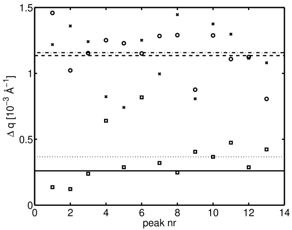
Figure 3.8: Peak width of thirteen 421 reflections from individual scattering LaB₆ domains. The sample-to-detector distance was $3736.7\mathrm{m}\mathrm{m}$, and a vertical detector position corresponding to the 400 reflection family of Cu at a X-ray energy of $52\mathrm{k}\mathrm{eV}$ was used (vertical center position of the detector was $1095\mathrm{m}\mathrm{m}$ above the direct beam). Widths in the three directions of the individual peaks are plotted as: $\Delta q_{x}$ ($\times$), $\Delta q_{y}$ (o) and $\Delta q_{z}$ ($\square{}$). Averages over the widths in the three directions are plotted as: $\langle\Delta q_{x}\rangle$ (dashed line), $\langle\Delta q_{y}\rangle$ (dash-dotted line) and $\langle\Delta q_{z}\rangle$ (dotted line). The theoretical mean size broadening (equal in all three directions) is plotted as: $\langle\Delta q_{\text{size}}\rangle$ (full line).

The mean values and differences, linearly and quadratic, from the theoretical size broadening are given in table 3.2. These numbers for $\bm{q}_{x}$ and $\bm{q}_{y}$ can be compared to the limits given in equation 3.14.

The range of the measured experimental broadening in the $\bm{q}_{y}$-direction overlap with the theoretical calculated range, and indicates that the real experimental broadening is close to the theoretical lower limit.

The range of measured experimental broadening in the $\bm{q}_{x}$-direction likewise overlap with the theoretical range, but in this case the measurement indicates that the real experimental broadening is close to the upper theoretical limit.

The observed experimental broadening in the $\bm{q}_{z}$-direction is very close to the resolution as defined by the rocking angle interval. It is therefore not possible to evaluate the intrinsic broadening in this direction, but only to observe that it is seen to be small.

The analysis above only set limits on the experimental broadening. If a true deconvolution is to be performed, a better method for characterizing the experimental broadening has to be devised. In the following scientific cases it will however be shown that much can be learned form the simple estimates of the experimental broadening.

	$\langle\Delta q\rangle$	$\langle\Delta q\rangle-\langle\Delta q_{\text{size}}\rangle$	$\sqrt{\langle\Delta q\rangle^{2}-\langle\Delta q_{\text{size}}\rangle^{2}}$
	$[10^{-4}\rAA]$	$[10^{-4}\rAA]$	$[10^{-4}\rAA]$
$q_{x}$	11.3	8.7	11.0
$q_{y}$	11.6	9.0	11.3
$q_{z}$	3.7	1.1	2.6

Table 3.2: Mean width of the 13 reflections, as shown in figure 3.8, in the three reciprocal space directions, $\langle\Delta q\rangle$. Included is the linear and quadratic differences between the measured widths and the theoretical size broadening $\langle\Delta q_{\text{size}}\rangle=2.6\cdot 10^{-4}\rAA$.

3.6 Data analysis

One or multiple 3D intensity distribution maps are obtained for each experiment. These datasets can be seen as 4D movies. The major challenge with respect to data analysis is how to gather relevant physical information from such large dimensional datasets.

As the broadening of the reflection is mainly in the azimuthal directions, the major technique for getting an overview of the intensity distribution is a projection onto the azimuthal plane.

Projections in one azimuthal direction over small parts of the perpendicular azimuthal direction have also been used, in cases where the radial (strain) information was analyzed.

Such 2D projections give a good overview of time/strain dependencies when arranged in tables.

Projections onto the radial direction carry information on the distribution of strain in the illuminated part of the grain (equivalent to traditional line broadening measurements). Such projections have been used for defining mean strain in the grains, and for comparing to the present line broadening-based results.

The background for the projections are rebinning of detector-pixel-data to the reciprocal space. The rebinning method used is presented in section 3.6.1. Section 3.6.2 presents the projection methods.

The main results of the technique are the properties of the observed single individual peaks. The analysis method used on these peaks is presented in section 3.6.3.

To gather statistical information on the observed cloud of enhanced intensity, and further information on the radial position of the individual peaks, a statistical analysis method has been devised, this is presented in section 3.6.4.

The general technique of converting the integrated intensity to volume of the scattering entity is finally presented in section 3.6.5.

3.6.1 First order rebinning

The problem of converting data obtained as pixels on a 2D detector to pixels in reciprocal space, or equivalent to angular space defined by pixels in a $\eta,2\theta$ coordinate system, is general for many applications of area detectors. The major problem is that a square pixel on the detector does not corresponds to a square pixel in reciprocal space, and that the shape and size of the pixel in angular space depends on the position of the pixel on the detector (figure 3.9 illustrates the differences in the case of the present setup).

Multiple software packages (such as [fit2d]) exist that are able to perform the general transformation, known as rebinning. The geometry of the present setup does, however, seems to give problems with FIT2D as the beam center is located far outside the image obtained. A first order rebinning scheme has therefore been used.

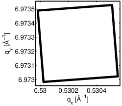
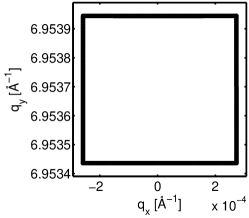
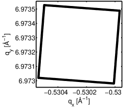
Figure 3.9: The mapping of one pixel squared on the detector onto the $(\bm{q}_{x},\bm{q}_{y})$-plane for three horizontal pixel positions. Geometrical parameters are chosen within typical values of the actual setup. The mapped pixel are located at (left to right) pixel nr. $-1000$, $0$, $1000$ with respect to the horizontal beam center, and vertically close to the position of the 400 reflection for Cu.

The differences in area in reciprocal space between the different pixels are minor, as the detector (and more important the interesting reflection) only covers a small angular range in the present case. This can also be seen on figure 3.9, where the differences are illustrated in the extreme case.

For the typical case (as represented in the data presented in acta) the maximal difference in the size of the voxels that corresponds to the pixels in the relevant region was calculated. In the azimuthal direction, $\bm{q}_{x}$, the change in length is at most $0.33\%$ of the minimum length, and in the radial direction, $\bm{q}_{y}$, the change is at most $0.05\%$ of the minimum length. In the other azimuthal direction $\bm{q}_{z}$ the size is constant. This gives a maximal difference in the volume of the voxels of $0.4\%$, and a first order rebinning scheme, which does not take this volume difference into account, is therefore appropriate.

The rebinning is not performed separately but is integrated into the projections as described in the following.

3.6.2 Projections of reciprocal space

Based on a data-set that have been rebinned to reciprocal space, projections are trivially done as a sum over voxels in the appropriate directions.

The general “first order rebinning” based projections are performed in the following way:

• Define the bins of the final projected intensity distribution:
  The bins are defined using the average pixel position in the selected region, in the $\bm{x}$ or $\bm{y}$-directions for the projections onto the radial direction or azimuthal plane respectively.

• For all voxels in the data set, calculate the $\bm{q}$-position.

• For all voxels find the closest bin in the final projection, add the intensity to this bin, and record that a voxel has been added to the bin.

• For each bin in the projection normalize by the number of added voxels to that bin.

Azimuthal projection

Projections onto the azimuthal plane have been done in two ways; the proper projection based on first order rebinning as described above, and an even simpler projection, based directly on the detector pixels.

The latter case is based on the fact that the horizontal plane of the detector is approximately in the $\bm{q}_{x}$-direction, hence a good approximation to the projection onto the azimuthal direction is obtained by summing over the columns of the detector pixels.

In the $\bm{q}_{x}$-direction this is very accurate, as the change in $\bm{q}_{x}$-position of the pixels over one column is much smaller than the bin size of the final projection. However, the $\bm{q}_{z}$-position of a pixel depends directly on the $2\theta$ position of the pixel (according to equation 3.7) and it is found that by just summing over columns some voxels might end up in the wrong bin in the projection. The error is however minor, and no significant differences are observed between the two projection types.

Generally the proper projection has been used for the large azimuthal projections (as the one in figure 3 in acta), and the simple projection for small projections (as the ones presented e.g. for reproducibility in section 3.7).

Radial projection

All integrated radial peak profiles reported in this study (as the one in figure 4.1) have been calculated using the first order rebinning technique.

The radial peak profiles are normally fitted (by least square fitting) using either a split pseudo-Voigt or normal pseudo-Voigt function. The pseudo-Voigt function is a weighted sum of a Gaussian and Lorentzian function (for a discussion of this function see [Enzo1999]). The normal pseudo-Voigt function has one parameter describing the width of the peak (in the version used the parameter is the full width at half maximum). In contrast the split pseudo-Voigt function has two width parameters, one giving the half width of the lower (with respect to the maximum) part, $\Delta_{1}$, and one giving the half width of the upper part, $\Delta_{2}$ (see figure 3.10). This can therefore be used for fitting asymmetric peaks. The two width parameters for the split pseudo-Voigt are normally added ($\Delta_{1}+\Delta_{2}$) to give the full width at half maximum, and subtracted ($\Delta_{1}-\Delta_{2}$) to give a measure of the asymmetry.

As quantitative results are derived from the radial peak profiles, it is important to know if the first order rebinning scheme distorts the peak profile.

Figure 3.10: Illustration of the split pseudo-Voigt function. Indicated are the two “half width at half maximum” parameters ($\Delta_{1}$ and $\Delta_{2}$), maximum position ($x_{\text{max}}$), maximum value ($I_{\text{max}}$), and half maximum ($I_{\text{max}}/2$).

To investigate this a detector image of a known radial peak profile was calculated. The peak profile is assumed to be constant in the azimuthal directions and to be described by a split pseudo-Voigt function in the radial direction. Typical parameters for the geometry of the setup and peak profile were used. To simplify the calculation the parameters of the peak profile, were converted to angular units, and the peak described as function of the scattering angle, $f(2\theta)$. The intensity in each pixel, $I_{\text{pixel}}$, was calculated as:

$$I_{\text{pixel}}=\iint_{\text{pixel}}f(2\theta(x,y))\frac{\partial(2\theta,\eta)}{\partial(x,y)}dxdy$$ (3.15)

where the functions $2\theta(x,y)$ and $\eta(x,y)$ are given by equation 3.1. The integration was carried out numerically.

The simulated image was treated in the same way as the normal data, and the simulated parameters and parameters found by the fitting were compared:

Parameter	Relative difference between fitted and simulated parameter
Peak position	$1.5\cdot 10^{-4}\%$
Full width at half maximum	$0.15\%$
Asymmetry	$0.7\%$

From this it is concluded that the first order rebinning scheme does not introduce any significant errors in the relevant parameters of the resulting radial peak profile.

3.6.3 Single peak analysis

Individual peaks have been identified either from the raw 3D data sets, or more frequently from azimuthal projections.

The position of the maximum, $\bm{q}$, the full width at half maximum (FWHM) in the three directions, $\Delta\bm{q}$, and the integrated intensity, $I$, have been found for the individual peaks.

The analysis is based on the full 3D intensity distribution in reciprocal space, according to the following procedure:

• The voxel with maximum intensity was identified.

• Three one-dimensional intensity profiles were gathered (along approximately the $\bm{q}_{x}$, $\bm{q}_{y}$ and $\bm{q}_{z}$-directions) going through the maximum voxel, and not integrating in the other directions.

• A one-dimensional pseudo Voigt function plus a constant term were fitted (using least square fitting) independently to each of these three profiles (figure 3.11 show an example of such a set of three fits).

Figure 3.11: Example of fitting a single peak to three individual pseudo-Voigt functions along the three reciprocal space directions. Dots indicate measured intensities and lines the fit obtained, the horizontal line indicates the full width at half maximum. From acta.

The fits directly give the position of the maximum in reciprocal space and full width at half maximum of the peak in the three directions.

On figure 3.11 it is seen that the constant level in the two azimuthal directions ($\bm{q}_{x}$ and $\bm{q}_{z}$) are approximately the same, this indicates that the procedure in these directions correctly separates the cloud and the peak. It is also seen that the constant level in the radial direction ($\bm{q}_{y}$) is lower, in fact it is almost at the detector background level. The reason for this is that it is very hard to separate the cloud and the peak in this direction as both tend toward $0$. This has the consequence that the method has a tendency of overestimating the width in the $\bm{q}_{y}$-directions. The uncertainty on the width is mainly attributed to the uncertainty on the level of the cloud, and hence on the half maximum level. It can be estimated individually from the fits, by varying the constant level between the fitted values.

The integrated intensity in a peak is found from the fits to the peaks. It is assumed that the average constant level and peak height found in the azimuthal directions can be used in the radial direction. The uncertainty of the total intensity was estimated by varying the background level used and the peak height between the minimum and maximum fitted values and constructing the corresponding upper and lower limits of the intensity. The estimated uncertainty is $\approx 15\%$.

3.6.4 Statistical analysis of intensity distribution

By the methods presented in the previous sections (3.6.2 and 3.6.3) information can be gathered on the overall strain distribution in the illuminated grain, and on the strain in the individual scattering entities giving rise to the peaks. Information on the strain distribution in the material which gives the cloud is a very good complement to these data on the grain and the subgrains.

The problem with gathering information on the cloud is that it is very hard to locate parts of the cloud which have no influence from the superimposed peaks. A statistical method for analyzing the overall distribution of strains in the illuminated material has been devised to overcome this problem.

The algorithm of the technique is as follows (see also figure 3.12):

• All possible radial line profiles are gathered (that is, one for each pixel/bin in the azimuthal plane).

• For each profile the maximum intensity, $I_{\text{max}}$, is found.

• The $\bm{q}_{y}$-position of this maximum, $q_{y,\text{max}}$, is found.

• The $(q_{y,\text{max}},I_{\text{max}})$ pairs are binned into log-intensity bins of constant width.

• The mean $q_{y,\text{max}}$ value is finally calculated for each bin, together with the number of points in each bin.

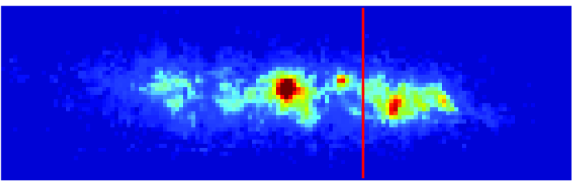
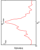
Figure 3.12: Ilustration of the statistical analysis method. The left part shows a raw detector image. The right part is the intensity profile along the red line indicated on the raw detector image. $I_{max}$ and $q_{y,max}$ are indicated on the plot.

An overview of the strain distribution is gathered by plotting the mean $q_{y,\text{max}}$ as a function of intensity (an example of such a plot is given in figure 3.18). The points at low intensity will correspond to an average over mainly the cloud, as the cloud has a much lower intensity than the peaks. In this way information on the average strain in the material giving the cloud can be obtained.

3.6.5 Volume calibration

The integrated intensity from a scattering entity is, as described in section 2.4.1, proportional to the volume of the scattering entity, under the assumption of kinematical scattering. This gives a possibility for finding the volume of both the part of the grain illuminated and the volumes giving rise to the individual peaks.

The proportionality constant is found by acquiring a diffraction pattern form a reference powder sample of the same material, using the same $hkl$ family [Lauridsen2000].

The general equation for the total diffracted intensity per angular unit from a powder was given in section 2.4.2. Equation 2.28 (on page 2.28) was derived under the assumption of an unpolarized X-ray beam, and a re-derivation is needed to generalize to other sources.

In the present case two facts simplify this need for a modification; the scattering angle is small due to the high energy and the reference measurement is only carried out over a small part of the Debye-Scherrer ring close to $\eta=0$. Both facts have the consequence that the polarization factor is very close to the one of vertical scattering from a horizontal polarized beam, which is constant, $P=1$. Equation 2.28 can therefore be used with $P=1$ as a model for the reference intensity measured on the detector.

The normalized reference intensity, $E^{\prime}_{\text{powder}}$, is defined as:

$$E^{\prime}_{\text{powder}}=\frac{E_{\text{powder}}4\sin(\theta_{hkl})\cdot 360\mathrm{\SIUnitSymbolDegree}}{I_{0,\text{powder}}V_{\text{powder}}m\Delta t},$$ (3.16)

with $I_{0,\text{powder}}$ being the intensity during the reference measurement and other symbols as in equation 2.28.

The volume of a scattering entity $(V_{\text{crystal}})$ can then be found as:

$$V_{\text{crystal}}=\frac{E_{\text{crystal}}\dot{\omega}\sin(2\theta_{hkl})}{I_{0}E^{\prime}_{\text{powder}}}$$ (3.17)

where $E_{\text{crystal}}$ is the integrated measured intensity of a reflection associated with the entity, $I_{0}$ the incoming intensity during the measurement and other symbols as in equation 2.27 (on page 2.27). The term $1/|\sin(\eta)|$ in equation 2.27 it replaced by $1$, as the rotation axis is perpendicular to scattering plane. It is assumed that the same material has been used for the reference powder as the one investigated, and that the powder measurement is carried out for the same reflection family as the one investigated.

In practice a highly deformed, cross rolled sample of the same metal is used as the reference material. A large slit opening is used for the measurement such that the diffraction pattern represents the average over sufficiently many grains that X-ray powder theory can be applied. Furthermore, the sample is put on a spinner to eliminate textural effects.

The biggest problem with this volume calculation scheme is that the incoming beam intensity has to be known, and the beam is, as was discussed in section 3.2.1, vertically bell shaped, giving a rather non-uniform incoming flux to different parts of the illuminated volume.

3.7 Reproducibility

The reproducibility of the 3D intensity maps has been tested many times, by repeating the mapping of a specific area of reciprocal space. The stress rig does only operates in displacement control, some stress and strain relaxation might therefore be observed during the measurements.

Figure 3.13 shows a reproducibility study conducted on a deformed Cu sample in connection with science (full details on the experimental conditions are given in the paper). A 3D map of the same region of reciprocal space was obtained three times at a tensile strain of $3.3\%$. Each map took $\approx 9$ minutes to obtain and was taken immediately after each other.

The logging procedure for the incoming intensity was unfortunately not working properly when this dataset was obtained. Therefore no intensity normalization has been applied; the total scattered intensity in the three maps are however almost constant (within $0.3\%$), indicating a stable beam.

It is seen that the three maps comprise the same features, with only minor variations of the exact intensities. This demonstrates that the method gives reproducible results, within the time limits of these investigations, $\approx 30$ minutes.

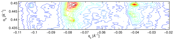
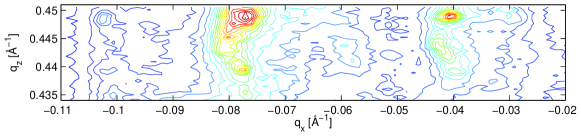
Figure 3.13: Reproducibility test in connection with science. A 3D reciprocal space map was obtained three times of the same part of the reciprocal space near a 400 reflection from a Cu sample deformed to $3.3\%$. Each part of the figure is a projection onto the azimuthal plane. Each map took $\approx 9$ minutes to obtain and was taken immediately after each other.

A longer investigation consisting of 40 repeated mappings, was conducted in connection with the study presented in newdyn. The total time spanned was $\approx 1.5\mathrm{h}$, and data sets were obtained immediately after each other. The datasets were normalized with the total incoming beam intensity, and the scattered intensity was constant within $\pm 6\%$. During the experiment a small stress relaxation was observed (the stress drop is $\approx 1.4\%$, and strain increment $\approx 0.2\%$).

A set of azimuthal projections are shown in figure 3.14, representing every sixth map. It is seen that the general features of the intensity distribution are stable on the time scale of the experiment. Some minor changes are observed, specially in the low intensity peaks, these effects are likely to arise from changes in the beam profile illuminating the sample, but could also be due to physical changes in the sample due to stress relaxation.

Figure 3.14: Reproducibility test in connection with newdyn. A 3D map was obtained 40 times of the same part of reciprocal space around a 400 reflection from a Cu sample deformed in tension to $1.8\%$ strain. Each part is a projection onto the azimuthal plane, with $\bm{q}_{x}$ horizontal and $\bm{q}_{z}$ vertical covering respectively $0.14\rAA$ and $0.006\rAA$. The datasets shown are separated by $\approx 13\mathrm{min}$ each.

These investigations demonstrate that the observed structures in the intensity distribution are reproducible.

3.8 Detailed arguments for the interpretation

The interpretation of the bright isolated spots as arising from individual dislocation depleted subgrains and of the cloud as arising from the dislocation-filled walls was introduced in section 3.1.2.

The argumentation for this interpretation has been developed in science, acta, icsma and almg. The arguments will in the following sections be reviewed and some points, which are less well documented in the papers will be substantiated. Experimental details given in the four papers will not be repeated here.

3.8.1 Observations from raw data

The first high resolution data was presented in science, and later a more detailed data set was presented in acta. The observations presented are general for all Cu and Al samples investigated.

The following data are from the experiment described in acta.

A copper sample was deformed to $2\%$ strain, and a grain with a $\langle 100\rangle$ direction close to the tensile direction was identified using the “Reflection based” technique described in section 3.3.1. The grain was found to be smaller than the beam, both by spatial scanning and a calculation based on the full scattered intensity. The grain was hence fully illuminated during the measurement. A full map of the reciprocal space around one 400 reflection, consisting of 300 $\omega$-slices, was obtained. The rocking interval was chosen to be $0.007\mathrm{\SIUnitSymbolDegree}$ corresponding to a size in reciprocal space of $\Delta q_{z}=8\cdot 10^{-4}\rAA$ hence close to the resolution in the other directions. An example of 9 $\omega$-slices is shown in figure 3.2 on page 3.2.

As the broadening is mainly in the azimuthal directions ($\bm{q}_{x}$ and $\bm{q}_{z})$) it is feasible to make a projection of the full 3D intensity distribution onto this plane (for details about this projection see section 3.6.2). The result of such a projection is a 2D map of the azimuthal spread, where the degree of freedom of strain has been integrated out. This projection is shown, for the full dataset, in figure 3.15. With the contour levels used the map comprises isolated peaks (corresponding to the ones seen in the raw data), large islands and a rather smooth cloud of intensity, well above the detector background level. In the insert it is seen that the islands are composed of individual peaks, some of them partly overlapping.

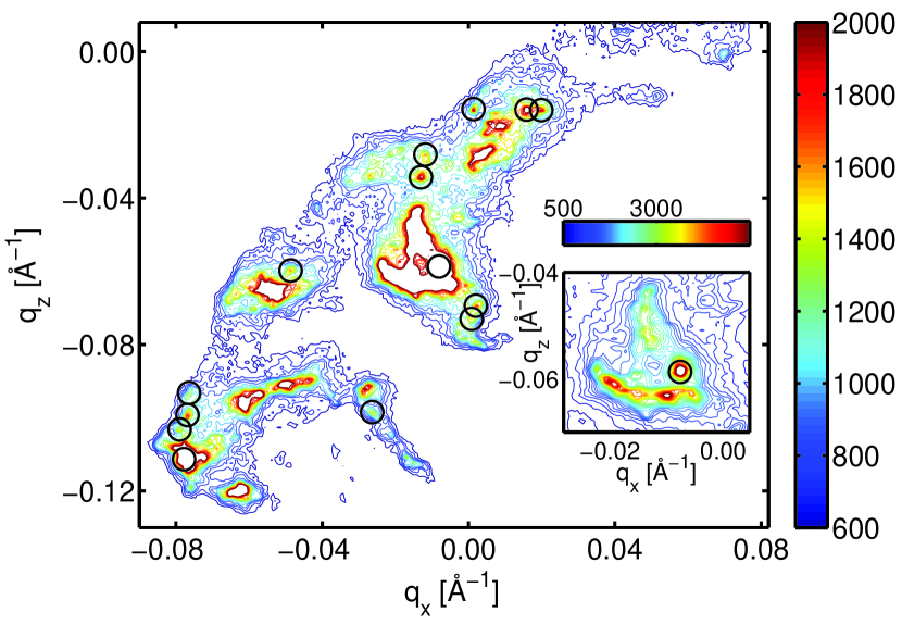
Figure 3.15: Projection of the 3D reciprocal space intensity distribution onto the azimuthal plane $(\bm{q}_{x},\bm{q}_{z})$. The color scale of the contour lines represents integrated intensity in units of detector counts. The insert is a zoom on the high intensity part around $(q_{x},q_{z})=(-0.01\rAA,-0.06\rAA)$ with different contour lines and color scale. The circles indicate the position of $14$ individual peaks selected for a statistical analysis as presented is section 3.8.2. From acta.

3.8.2 Single peaks

The properties of the individual peaks were initially reported in science and analyzed in greater detail in acta.

14 individual peaks were selected for detailed analysis from the dataset presented in figure 3.15.

The peaks were analyzed in the manner presented in section 3.6.3 obtaining the following properties: Position in reciprocal space, full width at half maximum of the peak in the three directions, $\bm{\Delta}q=(\Delta q_{x},\Delta q_{y},\Delta q_{z})$ and integrated intensity of the peak. The integrated intensity was converted to a volume by the procedure described in section 3.6.5. Figure 3.16 show the width and volume data for the peaks.

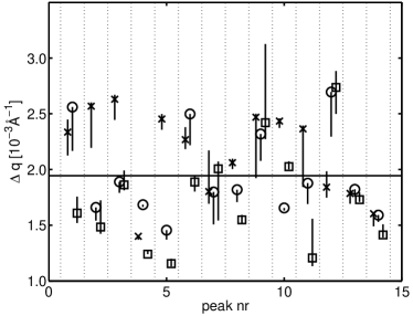
(a) The fitted full width at half maximum. Shown are the results for the three directions in reciprocal space $\Delta q_{x}$ ($\times$), $\Delta q_{y}$ (o), $\Delta q_{z}$ ($\square$). The full horizontal line indicates the average value of all peaks in all directions $\langle\Delta q\rangle\approx 1.9\cdot 10^{-3}\rAA$. The error bars are calculated from the uncertainty in the level of the diffuse cloud. The fitted value is in all cases an upper limit for the width in the $\bm{q}_{y}$-direction.

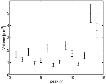
(b) Volume. The relative uncertainty is estimated to be $\approx 15\%$, whereas the uncertainty on the absolute scale of the volume is $50\%$. The last two data points are from peaks in the islands of enhanced intensity.

Figure 3.16: Properties of the 14 individual peak as shown on figure 3.15, as a function of peak number. From acta.

Volume

The mean volume from the 12 first, well-separated, peaks are $\langle V\rangle=1.4\mathrm{\SIUnitSymbolMicro}\mathrm{m}\mathrm{{}^{3}}$, corresponding to an equivalent sphere diameter of $\langle d\rangle\approx 1.4\mathrm{\SIUnitSymbolMicro}\mathrm{m}$. The width of the last two peaks is below the average width of the full set of peaks although the volume is larger. This indicates that the peaks do not arise from overlapping peaks from different regions. They do either come from larger dislocation-free regions, or they are from a part of the grain which is closer to the center of the vertical beam profile.

Compared to TEM investigations on similar polycrystalline systems (e.g. [Essmann1963; hansen2001] and figure 1.3) it can be seen that the length scale found above is comparable to what is reported for the dislocation-depleted regions in the dislocation structure (the subgrains).

Quantitative cell size measurements exist on single Cu crystals [Gottler1973]. Estimating the equivalent single crystal resolved shear stress by correcting for the grain size strengthening, it is possible to compare our polycrystalline data to the single crystal data [ acta]. It is found that the subgrain size in single crystals deformed to the resolved shear stress obtained here is $\approx 2\mathrm{\SIUnitSymbolMicro}\mathrm{m}$. This is in good agreement with what we observe. Furthermore, it is known that the distribution of sizes of the dislocation-free regions are wide (e.g. [Huang1998]), consistent with the observation of larger scattering regions.

Dislocation density

The mean width of the peaks in all three directions is $\left<\Delta q\right>\approx 1.9\cdot 10^{-3}\rAA$, not far from the instrumental resolution as reported in section 3.5.

A large dislocation density would give rise to a substantial broadening of the peaks, this indicates that the dislocation density is low in the scattering regions; consistent with the interpretation as a diffraction signal from the subgrains.

Spatial correlation

The connection between the individual peaks and the spatial position in the grain was investigated as part of the data obtained for science. A number of (small) reciprocal space maps were obtained at a fixed tensile strain of $4.07\%$, while translating the sample with respect to the beam. The translation was by steps of $2\mathrm{\SIUnitSymbolMicro}\mathrm{m}$ both in the $\bm{x}$- and $\bm{y}$-direction. For this particular experiment the beam size was $14\mathrm{\SIUnitSymbolMicro}\mathrm{m}$ by $14\mathrm{\SIUnitSymbolMicro}\mathrm{m}$.

In figure 3.17 projections onto the azimuthal plane are shown, as function of displacement from the position where the grain nominally is centered with respect to the beam.

The important thing to notice is that each peak seems to be associated with one spatial position in the grain as the intensity in all cases seem to describe the intensity behavior of a bell-shaped beam profile. The beam is assumed to be bell shaped in both the horizontal and vertical directions due to the small size (see figure 3.4). Information on the spatial position of the scattering entities, can in principle, be derived from such scans [poulsen04:bog; Lauridsen2001].

That the peaks seem to be associated with only one spatial position in the grain strengthens the interpretation as a signal from subgrains.

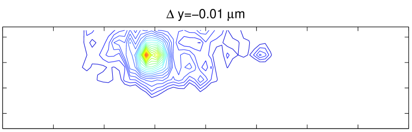
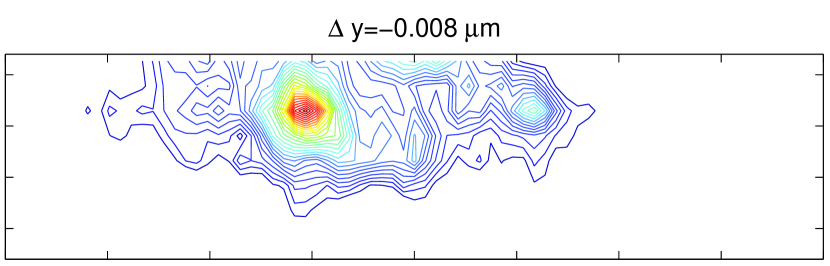
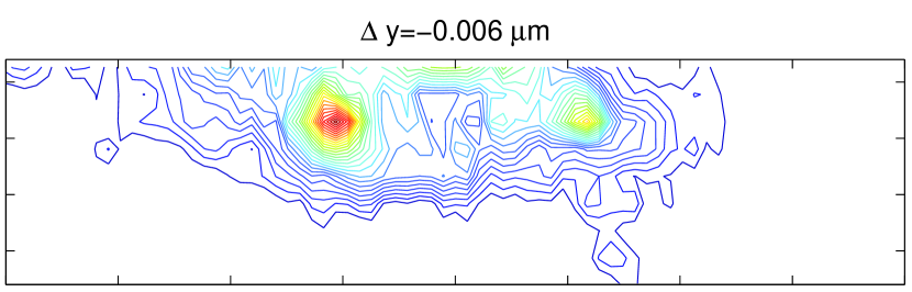
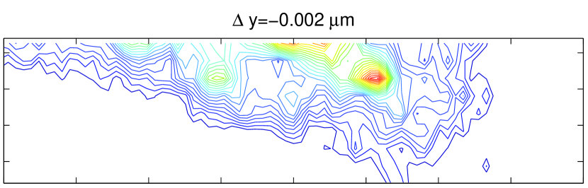
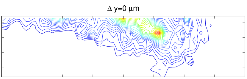
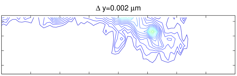
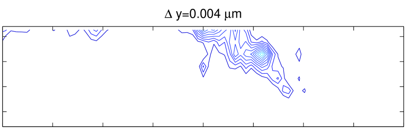
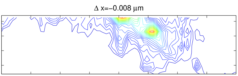
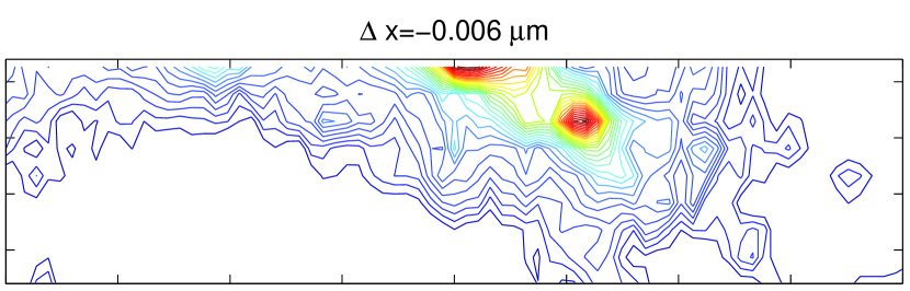
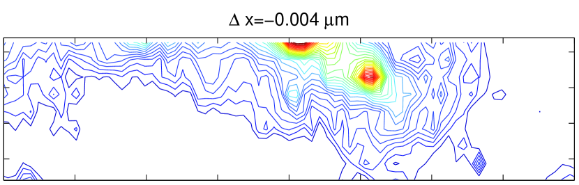
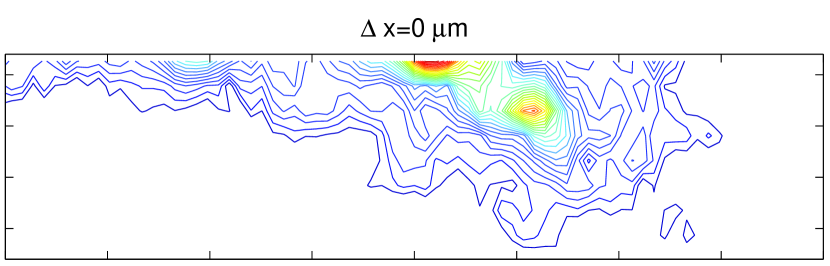
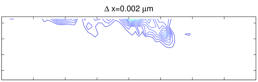
Figure 3.17: Azimuthal projections of 3D maps obtained at different positions with respect to the center of the grain. Each projection covers horizontally $0.08\rAA$ and vertically $0.02\rAA$. Full information on the experimental conditions are given in science.

3.8.3 The diffuse cloud

The diffuse cloud was in science tentatively interpreted as coming from the dislocation-rich walls in the dislocation structure. This interpretation was based on the fact that a large dislocation density will give rise to a broad strain and orientation distribution, hence to a signal in the reflection as the observed cloud. This interpretation has been substantiated firstly by an analysis of the mean strain in the material giving rise to the cloud [ icsma] and secondly by measurements on a system having a dislocation structure similar to the walls [ almg].

Statistical analysis of intensity distribution

The statistical analysis method presented in section 3.6.4 was applied to the data set presented in icsma. The grain analyzed is from the same Cu sample and same conditions ($2\%$ tensile deformation) as the one investigated in the previous sections.

Figure 3.18 shows the results of the analysis.

What can be observed is that a strong correlation exists between the maximum intensity and the radial position of the maximum. The dislocation-rich walls in a dislocation structure are, according to the composite model of Mughrabi1983, subjected to a forward stress (relative to the mean stress of the grain), and the dislocation-free subgrains to a back stress. If the model is true, and the interpretation of the cloud is true, a correlation as the one observed, would be the consequence [ icsma].

This is not a direct proof of the correlation between the walls and the cloud, but as other results shown that subgrains are subjected to a backwards strain see section 4.2 and [ acta], it significantly strengthens the hypothesis.

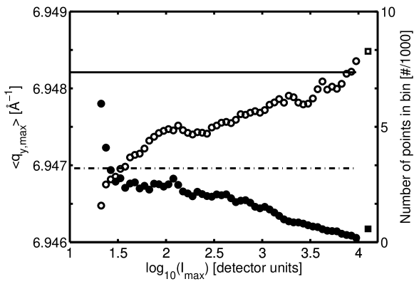
Figure 3.18: Position of the maximum intensity ($q_{y,\text{max}}$), along lines in the $\bm{q}_{y}$-direction through the 3D intensity distribution, as a function of maximum intensity ($I_{\text{max}}$). Each average $q_{y,\text{max}}$ marked by a circle $(\bigcirc)$ is taken over a small interval in intensity. The square $(\square)$ indicates the average $q_{y,\text{max}}$ position of all maxima with an intensity higher than $10000$. Corresponding filled symbols indicate the number of points in each intensity bin. The horizontal full and dash-dotted lines indicate the maximum and average of the integrated radial peak profile, respectively. From icsma.

Non-cell-forming metals

Measurements on a non-cell-forming AlMg alloy (aluminum + $4\%$ magnesium) were performed at different strains (experimental procedures and further results are presented in almg).

By TEM it was found that the dislocation structure, even after $10\%$ tensile deformation, was rather homogeneous. Figure 3.19 shows examples of electron micrographs. Figure 3.20 shows a comparison of raw $\omega$-slices obtained on the AlMg sample and a Cu sample strained equivalently. No distinct peaks are seen in the data from the AlMg sample. Projections onto the azimuthal plane of the obtained reciprocal space maps (as shown in figure 3.21 and figure 4 in almg) likewise show no distinct peaks, but some smooth large-scale intensity variations exists.

This indicates that a random tangle of dislocation gives a smooth intensity distribution similar to the cloud observed from cell-forming materials. Furthermore it shows that no clear peaks are observed when no subgrains are present, substantiating the interpretation of the peaks and cloud observed for copper.

A

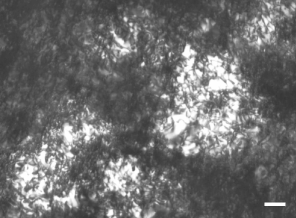
B

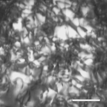
Figure 3.19: Transmission electron micrographs on a grain in a $10\%$ deformed AlMg sample. The grain is oriented $9\mathrm{\SIUnitSymbolDegree}$ from the $\left[100\right]$ orientation. Scale bars represents $200\mathrm{n}\mathrm{m}$. A) The developed high density of dislocations. B) High magnification view, shows a uniform distribution of dislocations. From almg.

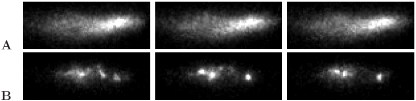
Figure 3.20: Raw $\omega$-slices. Part A: AlMg, Part B: Cu. Cu data are from the dataset presented as Grain I in section 4.2 (also presented in acta) and the AlMg data are from the dataset presented in almg (see also table 4.1). Read from left to right the images show consecutive $\omega$-slices. The images cover the same number of pixels but due to the difference in scattering and rocking angle the angular ranges covered is different, they cover $0.49\mathrm{\SIUnitSymbolDegree}$ (AlMg) and $0.42\mathrm{\SIUnitSymbolDegree}$ (Cu) in the azimuthal (horizontal) direction, $0.041\mathrm{\SIUnitSymbolDegree}$ (AlMg) and $0.039\mathrm{\SIUnitSymbolDegree}$ (Cu) in the radial (vertical) direction and is integrated over (rocking angle) $0.003\mathrm{\SIUnitSymbolDegree}$ (AlMg) $0.0067\mathrm{\SIUnitSymbolDegree}$ (Cu). From almg.

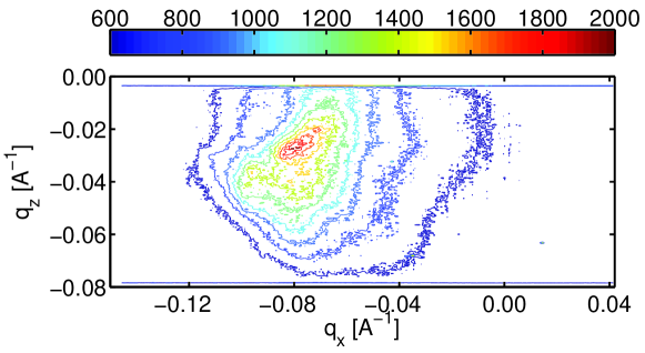
Figure 3.21: Projection of a partial 3D reciprocal space map of the 400 reflection from an AlMg sample deformed to $4.2\%$ in tension. From the data presented in almg.

3.9 Comparison to other techniques

High Angular Resolution 3DXRD can be compared to other techniques on a number of parameters. The technique is fundamentally a 3D reciprocal space mapping technique, and should be compared to equivalent methods. On a general level the technique has to be compared to other techniques which are able to measure elastic strains and orientations of individual subgrains in a deformation structure.

A advantage, that the technique inherits from the general 3DXRD principle, is the possibility for investigating individual grains deeply in the bulk of a polycrystalline sample. It may be debated to what extend this is important for the investigation of deformation structures. The use of polycrystalline samples has the advantage that grains of multiple orientations can be investigated in the same sample, and that the grain size limits the illuminated volume along the beam. This eliminates the need for complications such as the conical slit [Nielsen2000] or wire scanning [Larson2002].

The penetration power, due to the high energy, is clearly an advantage over traditional X-ray techniques. Copper $K_{\alpha}$ X-ray radiation has an attenuation length of $\approx 22\mathrm{\SIUnitSymbolMicro}\mathrm{m}$ in copper whereas the here used X-ray radiation with an energy of $52\mathrm{k}\mathrm{eV}$ has an attenuation length of $0.47\mathrm{m}\mathrm{m}$. This ensures that true bulk informations are gathered.

Reciprocal space mapping

Traditional 3D reciprocal space maps are acquired point-by-point using an analyzer crystal (e.g. [Fewster1995; Murphy2001]). This allows for a better resolution in some reciprocal space directions, e.g. along the diffraction vector as in Murphy2001. The disadvantage of such techniques is that 3 degrees of freedom have to be scanned to obtain a full 3D reciprocal space map.

The use of a 2D CCD detector clearly is an advantage with respect to acquisition time, as only one degree of freedom has to be scanned. The disadvantage of using a CCD detector is that its point spread function will influence the reciprocal space resolution. The severeness of the effect is determined by the sample-to-detector distance (as shown in equation 3.9a), and can be controlled by changing this. The contribution to the reciprocal space resolution from the detector is for the present setup of the same order of magnitude as the contributions from the beam properties (as can be seen in table 3.1 on page 3.1).

Strain measurements

The elastic strain (or equivalent the lattice spacing) in the individual subgrains have previously been measured by e.g. the convergent-beam electron diffraction (CBED) technique (e.g. [Kassner2002]), and can also be measured by the monochromatic version of the 3D crystal microscope [Levine2006].

The instrumental resolution in the $\bm{q}_{y}$-direction given by equation 3.14 (page 3.14a) corresponds to a width of $1.4$–$2.3\cdot 10^{-4}$ in strain. However, the position of the maximum of a peak from an individual subgrain can be determined better than this. We estimate the uncertainty to be $\pm 1/2$ pixel [ acta], corresponding to an uncertainty on strain difference of $0.7\cdot 10^{-4}$.

The uncertainty on the strain measurements on the 3D crystal microscope as reported in [Levine2006] is of similar magnitude. The CBED measurements reported in [Kassner2002] have an uncertainty of $\pm 1\cdot 10^{-4}$ for aluminum and $\pm 4\cdot 10^{-4}$ for copper.

This clearly shows that the X-ray based techniques have a better strain resolution. Further more, High Angular Resolution 3DXRD has the advantage that problems with stress relaxations near the surface are eliminated by measuring in the bulk.

Subgrain rotation

The width of the instrumental resolution in the $\bm{q}_{x}$-direction (as reported in equation 3.14) corresponds to an spread in lattice plane orientations of $0.006\mathrm{\SIUnitSymbolDegree}$ – $0.008\mathrm{\SIUnitSymbolDegree}$. This is again an upper limit on the observable orientation differences. In the other azimuthal direction much better resolution can be obtained on expense of acquisition time by decreasing the rocking interval size.

Orientation differences between different parts of a grain can be measured by TEM techniques to an accuracy of $0.3\mathrm{\SIUnitSymbolDegree}$ – $0.1\mathrm{\SIUnitSymbolDegree}$ [Liu1995; Huang2006]. High Angular Resolution 3DXRD provides, at least, an order of magnitude better angular resolution.

Summary

These comparisons show that the developed technique, on the selected parameters, has as good or better resolution as other existing techniques with respect to probing the properties of individual subgrains in a deformation structure.

The main disadvantage of the technique is that no spatial information are obtained. Spatial information could be obtained by spatial scanning techniques, but it would, as always, be at the expense of data acquisition time.

The main advantage, on the other hand, is the ability to perform relatively fast experiments on bulk structures. No other technique presently allows for investigation of the dynamics of individual bulk subgrains during deformation.

Chapter 4 Results and discussion

4.1 Introduction

High Angular Resolution 3DXRD was used for a number of experiments. The results provide new insight into the static properties of subgrains, and on the dynamics of the dislocation structures during deformation. Table 4.1 provides an overview of the experiments presented, and the sample materials used.

The main results have been reported in six papers, as indicated below:

science

presents the general technique and interpretation. The main scientific focus is on the dynamics of the subgrain structure during deformation (subgrain refinement), but a number of other issues are briefly touched upon.

acta

gives a thorough description of the technique and the single peak analysis method. The static properties of the subgrains, namely the distribution of elastic strain and dislocation density, are analyzed.

icsma

presents the statistical analysis method developed. The interpretation of the cloud is substantiated, and the average strain in the walls is discussed.

fda

summarizes the main results of the first three papers. The focus is on communicating the results in a less technical and more materials science-focused framework.

almg

presents measurements on a non-cell-forming alloy (AlMg). This study is in this thesis mainly used as evidence for the interpretation of the observed cloud (as presented in section 3.8.3).

newdyn

presents results from measurements during continuous deformation. The measurements complement the results on subgrain dynamics presented in science, and provide independent results on the stability of the subgrain structure during stress relaxation and offloading.

The results will be summarized in this chapter, collecting some of the fragmented results which have been separated over more than one paper. A number of results not yet included in any paper will also be discussed. Not all experimental details described in the papers will be repeated in this chapter.

The two first sections (4.2 and 4.3) deal with the static properties of the dislocation structure. The results from science to fda are combined. Two main issues are dealt with: the distribution of elastic strain in the dislocation structure, and the dislocation density in the subgrains.

Sections 4.4 and 4.5 deal with the dynamic properties of the dislocation structure probed by in-situ deformation experiments, the results from science and newdyn are combined. The first section (section 4.4) discusses the formation of subgrains during deformation of a fully recrystallized sample, and the possible consequences of ending a deformation. The stability of the overall structure is furthermore analyzed with respect to stress relaxation and off-loading. The process of subgrain refinement is discussed in the second section (section 4.5).

(a) List of the main data-sets used in this study.

(b) List of the sample types used for the experiments.

Table 4.1: Overview of datasets and samples.

4.2 Distribution of elastic strain

The radial broadening of the reflections from a plastically deformed crystal (e.g. a single grain within a polycrystalline sample), shows that some distribution of microscopic elastic strain exists in the crystal (see section 2.3.1). However no information is obtained on the spatial distribution of strains in the crystal. The microscopic strains may e.g. be described by the same distribution in any region of the crystal, or differences may exist between different parts of the dislocation structure. An example of the latter is the differences between subgrains and walls as suggested by the composite model (see page 2.3.1).

High Angular Resolution 3DXRD allows for a direct determination of the mean elastic strain in the individual subgrains, using the single peak analysis method (section 3.6.3). The analysis does also gives a limit on the width of the elastic strain distribution within each individual subgrain. Furthermore the mean elastic strain in the wall material can be analyzed by the statistical analysis method presented in section 3.6.4.

The main part of the results presented in this section has been reported in acta and icsma.

Results

The two samples investigated were deformed to $2\%$ plastic strain in tension, from a fully recrystallized state. All investigations were performed under load, with a fixed grip spacing (details on stress and strain are provided in table 4.1). The grains selected have the tensile axis close to (within $10\mathrm{\SIUnitSymbolDegree})$ a $\left<100\right>$ orientation. Grains were selected using the methods presented in section 3.3. This grain orientation ensures that the morphology of the deformation structure is a simple cell structure (see section 1.1.2).

The choice of grain orientation furthermore allows for comparison to the results by Ungár and co-workers [Ungar1984; Ungar1984b; mughrabi86,
Ungar1991]. They report asymmetrical line profiles (see section 2.3.1) from $[001]$-orientated single crystals deformed in tension. Their lowest degree of deformation is to a true tensile stress of $64.2\mathrm{M}\mathrm{Pa}$ at a tensile strain of $2.8\%$ [mughrabi86]. This is not far from the $2\%$ tensile deformation reported here, where for grains I and II we find a tensile stress of $67\mathrm{M}\mathrm{Pa}$ when correcting for the grain size hardening by use of the Hall-Petch relation [ acta]. We will hence in the following discussion compare to their results.

The datasets on grain I and II each consist of a full map of one $400$ reflection. The reflections are from the $\left\{100\right\}$ planes which are close to being perpendicular to the tensile axis (the axial case in the notation introduced in the section on “asymmetric line broadening” on page 2.3.1). The grains are from the same sample, and were found by the reflection-based technique (section 3.3.1); the full crystallographic orientation is hence not known.

The dataset on grain III is from a different sample investigated at a later beamtime. The full orientation of the grain was found by the GRAINDEX method (see section 2.5.1), this allows one to obtain reciprocal space maps for more than one reflection from the grain. Two $400$ reflections were investigated, one being the axial case as above, and one a side case (having the scattering vector, close to, perpendicular to the tensile direction). The reciprocal space maps were not covering the full azimuthal spread of the reflection.

Integrated radial peak profile

The average elastic strain distribution in the illuminated part of the grains, is analyzed by projecting the obtained 3D reciprocal space map onto the radial direction (see section 3.6.2) to obtain the integrated radial peak profile. Figure 4.1 shows such a profile for grain I.

The profiles have been characterized by fitting to a split-pseudo-Voigt function (see section 3.6.2), and some statistical calculations. The main parameters derived from the radial profiles are the mean value, the position of the maximum, the peak width and the asymmetry. The parameters for the individual grains investigated are reported in table 4.2.

	Grain I (axial)	Grain II (axial)	Grain III (axial)	Grain III (side)
$q^{\text{grain}}_{y,\text{max}}[\rAA]$	6.9480	6.9482	6.9470	6.9579
$\left<q_{y}^{\text{grain}}\right>[\rAA]$	6.9473	6.9470	6.9447	6.9588
$\Delta_{1}+\Delta_{2}[10^{-3}\rAA]$	6.4	5.5	9.4	8.5
$\Delta_{1}-\Delta_{2}[10^{-3}\rAA]$	0.8	1.4	2.8	-0.9

Table 4.2: Parameter for the integrated radial peak profiles, based on the 3D reciprocal space maps obtained under load for the three grains investigated. $\Delta_{1}$ and $\Delta_{2}$ are the half-widths of the lower and upper part of the profile respectively. $\Delta_{1}+\Delta_{2}$ is the full width at half maximum, and $\Delta_{1}-\Delta_{2}$ a measure of the asymmetry. Measurements on grains in the undeformed state suggest that the absolute position of the peaks from grain III might be slightly ($\approx 1.4\cdot 10^{-3}\rAA$) shifted to higher $q_{y}$-values.

It may be observed that each profile is asymmetric. In the axial cases the intensity falls off more slowly to the low-$q_{y}$-side and in the side case the slow decay is on the high-$q_{y}$-side. This is in agreement with what is reported by Ungar1984 on single copper crystals deformed in tension.

It is furthermore observed that the width, asymmetry and absolute position differ somewhat between the grains. This must be due to the inhomogeneities of the stress-fields at the grain level, especially for grain I and II which are from the same sample.

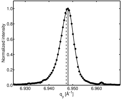
Figure 4.1: The integrated radial peak profile for grain I. Projection of the 3D reciprocal space intensity distribution onto the radial direction ($\bm{q}_{y}$). The full line is a fit to a split-pseudo-Voigt function. Vertical full and dash-dotted lines indicate the position of the maximum and the average of the profile, respectively. Adapted from acta.

Elastic strain in and between subgrains

The mean strains of 14 individual subgrains from grain I have been analyzed (results are reported in acta (as $q_{y}$-positions of maximum), and fda (as elastic strain)). The $q_{y}$-position of the maximum of the individual peaks, are found by the single peak analysis methods presented in section 3.6.3. Figure 4.2 shows the maximum $q_{y}$-positions of the individual peaks. Also shown is the position of the mean value and the maximum of the integrated radial peak profile for this grain.

Three important conclusions can be drawn from this data and from the peak width of the individual peaks (as reported in figure 3.16(a) on page 3.16(a)):

• The individual subgrains have different mean elastic strains.
  The distribution has a width of $2.9\cdot 10^{-4}$, if defined by twice the standard deviation of the peak positions.

• The mean value of the peak positions are shifted by a significant amount compared to the mean value of the integrated intensity profile.
  The difference corresponds to a reduction of the elastic strain with respect to the applied stress (a backwards strain) in the subgrains by $0.9\cdot 10^{-4}$, on average.

• The width of the elastic strain distribution inside the individual subgrains has an upper limit of $2.4\cdot 10^{-4}$.
  

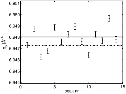
Figure 4.2: The fitted $q_{y,\text{max}}^{\text{subgrain}}$-positions for 14 isolated peaks as a function of peak number (same peaks as reported on figure 3.15 and 3.16). The uncertainty in the peak position is conservatively estimated to be $\pm 2.5\cdot 10^{-4}\rAA$. The average $q_{y}$-position of the individual peaks is $\left<q_{y,\text{max}}^{\text{subgrain}}\right>=6.9479\pm 0.0003\rAA$, with a standard deviation on the positions of $\approx 1.0\cdot 10^{-3}\rAA$. The dashed-dotted horizontal line indicates the mean value of the integrated radial profile (as shown in figure 4.1) and the full horizontal line the maximum of the integrated radial profile. Adapted from acta

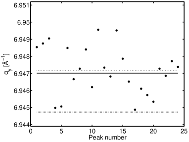
(a) Axial case. $\left<q_{y,\text{max}}^{\text{subgrain}}\right>=6.9472\rAA$

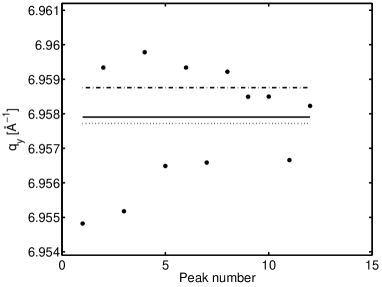
(b) Side case. $\left<q_{y,\text{max}}^{\text{subgrain}}\right>=6.9577\rAA$

Figure 4.3: The fitted $q_{y,\text{max}}^{\text{subgrain}}$-positions for single peaks from grain III (some of the peaks were identified by M. Prinz [Prinz2006]). The dashed-dotted horizontal line indicates the mean value of the integrated radial profile and the full horizontal line the maximum of the integrated radial profile (as given in table 4.2). The dotted horizontal line indicates the average $q_{y}$-position of the individual peaks.

An equivalent analysis on grain III shows very similar results for both the axial and the side case. Figure 4.3 shows the positions of the individual peaks in both the axial and the side cases. The distribution of mean strain of the subgrains is wide, with a mean value very close to the maximum of the integrated radial peak profile (compare table 4.2). The width of the individual peaks is furthermore similar to the values reported in figure 3.16(a).

Strain in subgrain boundaries

The technique does not allow for direct access of the strain in the subgrain boundaries. However, it was in section 3.8.3 argued that the observed cloud of enhanced intensity can be attributed to the walls.

The statistical analysis method (section 3.6.4) will give access to the mean strain in the walls if the correlation between wall material and the cloud is accepted. The method has been applied to grain II and the result is presented in figure 3.18 on page 3.18 (and in icsma). This analysis suggests that the walls are in-fact subjected to an enhanced elastic strain with respect to the mean strain in the grain (a forward strain), as the mean $\bm{q}_{y}$-positions at very low intensities indeed are below the mean value of the fully-integrated peak profile.

It should be mentioned that such an analysis requires measurements with very good counting statistics. Equivalent analyses on the other datasets show the same trend, but not as pronounced a backwards strain as the one observed in figure 3.18.

Discussion

The composite model by Mughrabi1983 predicts that strain differences exist between the subgrains and the walls. The asymmetry of peak profiles observed from plastically deformed crystals has been rationalized by use of this model, and a “decomposition scheme” has been developed [mughrabi86; Ungar1984; Ungar1984b] (see also section 2.3.1). The asymmetric peak is in this framework divided into two parts; one from the subgrains and one from the walls (see figure 2.2 on page 2.3.1). These parts have then been analyzed independently with respect to e.g. dislocation density.

The model/technique has been used in a number of studies, but has also been criticized. The existence of internal strains has e.g. been debated [Kassner2002; straub96].

The present technique gives the possibility for testing some of the assumptions and predictions from the composite model in a direct way.

Our results directly show that the predicted reduction in elastic strain in the subgrains exists on average. Similarly our measurements indicate that the enhancement of elastic strain in the walls exists.

The composite model predicts that the backwards strain in the subgrain, as observed in the axial case, is accompanied by a forward strain in the side case, due to cross contraction. This leads to a reversal of the asymmetry of the radial peak profile, as for the one observed for grain III in table 4.2. The magnitude of the forward strain in the side case is related to the backwards strain in the axial case by the Possion ratio [mughrabi86]. The ratio between the two strains can be calculated for grain III as (using values from figure 4.3 and table 4.2):

$$\frac{\left[\left<q^{\text{subgrain}}_{y,\text{max}}\right>/\left<q_{y}^{\text{grain}}\right>-1\right]_{\text{side}}}{\left[\left<q^{\text{subgrain}}_{y,\text{max}}\right>/\left<q_{y}^{\text{grain}}\right>-1\right]_{\text{axial}}}=-0.4.$$ (4.1)

The result is close to the Poisson ratio which is $0.42$ for a $\left<100\right>$ oriented single crystal [Landolt-Bornstein]. The observed ratio is seen to be consistent with the predictions of the composite model.

The backwards strain in the subgrains is furthermore found to be of the order of $10-25\%$ of the average elastic strain of the grain under load (as evaluated from the mean position of the integrated radial peak profile with respect to an undeformed sample). This corresponds well with the result by Ungár et al. where a back stress which is $12\%$ of the average flow stress is reported for the sample deformed to $26.2\mathrm{M}\mathrm{Pa}$ [Ungar1991].

It should be mentioned that Levine2006 recently have reported comparable results based on measurements on the 3D crystal microscope (as described in section 2.5.2). Their data are taken in the offloaded state, and only for the axial case.

Even as our results indicate that the composite model is conceptually correct, they also suggest that the results of the decomposition scheme for asymmetric peaks have to be re-interpreted. The result of the decomposition scheme applied to asymmetric integrated radial peak profiles is, as mentioned earlier, two well behaved peaks, one attributed to the subgrains and one to the walls (see figure 2.2). The analysis of the two peaks has been done applying traditional line profile theory. This corresponds to the implicit assumption that the major contribution to the broadening and shape of the peak attributed to the subgrains is the strain distribution within the subgrains and not among them.

Our results show that the distribution of strains between the subgrains is wider than the internal strain distribution in the subgrains. The analysis of grain I shows that the ratio of the two widths is $0.8$. As the estimate of the strain distribution within the subgrains is a conservative upper limit this ratio is probably even smaller.

To summarize, we suggest the following interpretation of the two peaks obtained by the decomposition method:

• The position of the peak corresponding to the subgrains represents the mean of the distribution of strains between the subgrains.
  A backward strain exists in a average sense

• The width of the peak corresponding to the subgrains, is highly influenced (if not dominated) by the distribution of strain between the subgrains, and hence does not represent the distribution of strains within the individual subgrains.

The results in this section show that performing 3D reciprocal space mapping at a high resolution can provide very important results regarding the internal elastic strain distribution in cell-forming metals. Furthermore the results provide a test of some of the fundamental assumptions in the interpretation of more traditional X-ray analysis such as line profile analysis.

4.3 Dislocation density in the subgrains

An other interesting parameter is the dislocation density inside the subgrains, $\rho$. The density of dislocations influences the flow stress of the individual subgrains, as $\tau\propto\sqrt{\rho}$, and hence needs to be understood for making flow stress models which take into account the in-homogeneity of the dislocation structure.

The decomposition scheme of asymmetric radial peak profiles, as discussed in the previous section and on page 2.3.1, has been used for evaluating the dislocation density in the subgrains and walls. Such measurements are e.g. reported in [Ungar1984; mughrabi86] where the ratio of dislocation density between the walls and subgrains is found to be of the order of 10. The findings however contradict some electron microscopy-based measurements [Argon1993; Haasen1993], where it is found that the dislocation density in the subgrains are “many orders of magnitude” smaller than in the walls.

Our results suggest, that the radial peak profile obtained from the composite model-based decomposition scheme, is in fact highly influenced by the distribution of strains between the subgrains. The peaks for the individual subgrains are substantially narrower, and hence indicate a lower dislocation density.

The ideal way to evaluate the dislocation density would be to utilize an appropriate theory or model which connects the dislocation density and dislocation configurations to the resulting 3D diffraction peak (or some projection of this). However, this is not possible within the time-frame of this study, as it would require a complete characterization of the instrumental broadening of the High angular Resolution 3DXED setup, allowing for deconvolution of the peaks obtained. Two approaches, avoiding this problem, will be discussed in the following (results also reported in acta).

A discussion will be given as to what can be learned on the basis of the upper limit of $1.7\cdot 10^{-3}\rAA$ on the mean radial width of the physical peaks (as was reported in the last section (see the footnote on page 2). The lack of full information on the peak shape will be treated by eliminating all parameters but the peak width from a line profile theory using literature values.

The results suggest that the dislocation density is very low and hence that “statistical” approaches might not be appropriate. A second approach has therefore been devised. This approach is based on direct calculations of the peak shape from a given dislocation configuration in a subgrain. Presently this analysis is restricted to one dislocation in the center of a subgrain, but in theory it should be possible to generalize the approach.

Density of redundant dislocations

A classical way to obtain information on dislocation density from integrated radial peak profiles is through a model for the micro-strain-distribution from some dislocation distributions. Such a model is then combined with the general theory for the Fourier coefficients associated with the radial peak profile (as discussed in section 2.3.1). This allows for a fit of the parameters of the dislocation distribution, based on the measured peak profile.

The results by Ungár and co-workers [Ungar1984; Ungar1984b; mughrabi86; Ungar1991] are obtained by use of the classical theory by Wilkens [Wilkens1970; Wilkens1970b]. The Wilkens’ theory is therefore used in the following analysis, as values reported by Ungár and co-workers then can be used for the calculations.

Wilkens introduces the concept of a restricted random dislocation distribution. A region where the dislocations follow a restricted random distribution can be divided into a number of sub-regions of equal size, with the same number of, randomly distributed, dislocations in each sub-region. The dislocations are not fully randomly distributed in the entire region, hence the name “restricted random”. It has been shown that such a dislocation distribution avoids the logarithmic divergence of the energy with crystal size, which is associated with a totally random dislocation distribution [Wilkens1970c].

The distribution is characterized by two parameters, the dislocation density, $\rho$, and the parameter $M$. Where $M$ is proportional to the average number of dislocations participating in the stress-screening configurations. A certain mixture of dislocation types (characterized by Burgers vector and direction) is assumed when the Wilkens’ theory is applied to the peak profile analysis. It is further assumed that the dislocation distribution, for each type of dislocation, consists of an equal amount of positive and negative Burgers vectors, hence the term “redundant dislocations”.

Our peak profiles do, as mentioned, not contain enough information to fit both parameters in a traditional Wilkens’ analysis. We have therefore chosen to fix the $M$ value. The Wilkens’ theory then predicts the width of the integrated radial peak profile as function of the dislocation density.

We have chosen to use the value of $M=1.60$ given in [Ungar1984] for a deformation which is comparable to ours. We furthermore assume the same mixture of dislocation types, allowing for use of the parameters describing the dislocation types given in [Ungar1984].

The limit of $1.7\cdot 10^{-3}\rAA$ on the width of the physical peak profile, is for a peak which is not integrated in the azimuthal directions. Wilkens’ theory predicts the shape of the azimuthally integrated radial peak profile. This possibly introduces an additional broadening of the peak, depending on the details of the 3D peak shape. Correction for this gives an upper limit on the azimuthally integrated radial peak profile of $2.6\cdot 10^{-3}\rAA$.

Based on this upper limit on the width of the integrated radial peak the dislocation density can be calculated. The parameters by Ungár and co-workers and the theoretical connection between the normalized $M$ factor and normalized half width given in figure 1 in [Wilkens1970] are used in the calculation. The resulting limit on the dislocation density is $12\cdot 10^{12}\mathrm{m}^{-2}$ substantially lower that the value of $22\cdot 10^{12}\mathrm{m}^{-2}$ reported by Ungar1984. It should be emphasized that our result is a very conservative upper limit on the dislocation density, and that the real dislocation density possibly is much lower.

Density of excess dislocations

Excess dislocations (that are dislocations not compensated by a dislocation of opposite Burgers vector nearby) will have a tendency to broaden the reflection in the azimuthal plane [Wilkens1984].

Two arguments which show that as little as one excess dislocation in a subgrain will lead to a visible “splitting” of the reflection, will be provided. Both arguments are based on considerations of one edge dislocation positioned in the center of a subgrain.

In the first model the dislocation is treated as a part of a symmetrical tilt boundary consisting of edge dislocations with a separation of the subgrain size $(D)$. Figure 4.4(a) illustrates this situation.

The angular difference between the two sides of such a boundary, $\beta$, is, as mentioned in section 1.1.1, given as $\beta=b/D$ where $b$ is the length of the Burgers vector ($2.55\mathrm{\SIUnitSymbolAngstrom}$ for $\left<110\right>1/2$ dislocations in the $\{111\}$ plane for Cu). Setting $D=1.1\mathrm{\SIUnitSymbolMicro}\mathrm{m}$ (the mean 2D length scale of the subgrains found in acta) results in $\beta=0.013\mathrm{\SIUnitSymbolDegree}$. If the two sides of the boundary can be considered as scattering, partly, incoherently this will directly lead to a splitting of the reflection in the azimuthal direction of $q_{\text{azimuthal}}\approx 1.6\cdot 10^{-3}\rAA$.

Figure 4.4: Illustration of the two models of one dislocation in the center of a subgrain. a) The dislocation is considered as part of a symmetrical tilt boundary. b) The dislocation is considered as being placed in the center of a cylinder with free boundaries.

The second model is based on the observation that subgrains with a volume of $\approx 1\mathrm{\SIUnitSymbolMicro}\mathrm{m}^{3}$ comprise $\approx 3000^{3}$ Cu atoms. This limited size makes it feasible to make direct calculations of the diffracted intensity from a 2D section of a subgrain. The atomic positions in such a section can be obtained from the elastic displacement field from the dislocation configuration.

The calculation is done on a cylindric fcc crystal with a dislocation in the center and free boundaries. Figure 4.4(b) illustrates this configuration. The cylinder is infinite in the $[100]$-direction with a diameter of $D$ in the perpendicular plane (comprising directions $[010]$ and $[001]$). The crystal is orientated such that the crystallographic coordinate system and the experimental coordinate system coincide. The edge dislocation in the center has a Burgers vector of $[011]1/2$. The direction of the dislocation line is the $[100]$-direction; hence it is not a mobile dislocation. With this geometry the position of the atoms can be calculated from the elastic approximation of the displacement field for one dislocation in a cylindrical crystal with free boundaries, as determined by leibfried49. The elastic and crystallographic parameters were chosen to be those of Cu.

The reflections associated with such a system are essentially two-dimensional due to the translation symmetry of the crystal. The intensity distribution can therefore be calculated from the atomic positions in a single (100) plane; the calculation is 2D both in real and reciprocal space. The diffracted intensity distribution is obtained by standard kinematic diffraction theory as described in section 2.1 using equation 2.3 and 2.4 (on page 2.4) with the atomic scattering factor set to one.

Figure 4.5 shows the resulting intensity distribution within the 040 reflection. It may be observed that the distribution splits into three parts each separated by $\approx 1.3\cdot 10^{-3}\rAA$ with the major splitting in the azimuthal $\bm{q}_{z}$-direction.

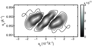
Figure 4.5: Atomistic simulation of the intensity distribution within the 040 reflection for a quasi 2D fcc crystal with one 1/2[011] edge dislocation in the center. In the calculation elastic and crystallographic properties of Cu were used and the boundaries taken as free. The cylindrical domain had a diameter of $3000$ inter-atomic distances ($\approx 1.1\mathrm{\SIUnitSymbolMicro}\mathrm{m}$) corresponding to an area of $0.9\mathrm{\SIUnitSymbolMicro}\mathrm{m}^{2}$, giving a dislocation density of $1\cdot 10^{12}\mathrm{m}^{-2}$. The gray-scale bar is in dimensionless units.

These two models of a single dislocation in a subgrain, show that High Angular Resolution 3DXRD might be sensitive to as little as one excess dislocation in a subgrain, as it will lead to a visible split of the associated peak. It should be noted that the orientation of the dislocation with respect to the scattering vector, determines the visibility of the dislocation in the diffracted signal.

We have generally not found such split peaks in the static investigations [ acta], indicating that the existence of single excess dislocations is rare.

Figure 4.6: Excerpts form larger azimuthal projections of reciprocal space maps taken at increasing strain. These are shown from left to right as a function of external strain (with strain increments relative to the first map shown). The peak followed split into two parts (as indicated by the arrow) and then recombines. Color scale and contour lines are identical to those on figure 4.14. Adapted from science.

A stepwise loading experiment has been performed (see section 4.5, “stepwise deformation” in table 4.1 and science). The peaks from a number of subgrains were followed in-situ during stepwise straining. During this experiment we did observe several peaks which split into two at some strain and then recombine at a later strain step. Figure 4.6 shows such a sequence. The interpretation is that a single (or a few) dislocation(s) got trapped in the subgrain investigated, and that it/they at a later deformation stage got released.

4.4 Formation and stability of subgrains

Investigations of subgrains during continuous deformation are possible using High Angular Resolution 3DXRD. Such experiments make it possible to address questions about the formation and stability of the dislocation structures.

Experimentally, the specifications of strain rate, wished time/stain resolution, acquisition time for one detector image ($\omega$-slice), and the size of the 3D maps are highly interlinked. Typically the 3D maps are highly truncated in the $\bm{q}_{z}$-direction in order to obtain a reasonable time/strain resolution.

Two experimental scenarios have been used. In the simplest case; one focuses the beam on a particular grain, but does not try to keep the beam at a precise position within the grain. As function of time the same reflection from a grain can then be mapped, but not necessarily the same part of the reflection. In the more challenging case one tries to keep the beam fixed with respect to a position within the grain and perhaps to compensate for macroscopic grain rotations leading to movement of the reflection.

In the following, two examples of such continuous deformation experiments will be presented. They both relate to studies of formation and stability of dislocation structures.

A fundamental limitation of TEM is (as mentioned in section 1.1.3) that the technique is ex-situ (unless thin films are investigated). The consequences of offloading and sample preparation for TEM investigations have been considered in the past (e.g. [Mughrabi1971; Young1967]). However, it is impossible to show by TEM if the dislocation structures observed after the deformation has ended are the same as the ones that existed during the deformation.

Fundamentally two very different scenarios for the consequences of terminating the deformation can be imagined. The structural formation may be a part of the plastic deformation process, the dislocations generating the structures dynamically while the sample deforms, and hence nothing dramatic happens at the end of deformation. Alternatively the subgrain structure might be the result of a relaxation process at the moment where the deformation stops, and therefore not be representative of the dislocation distribution which existed during the deformation.

It should be possible to distinguish between these two scenarios by continuous deformation experiments with the present technique.

The first experiment addresses the initial formation of dislocation structures as a fully recrystallized sample is continuously deformed, but does not address the consequence of ending the deformation.

The second experiment addresses the possible changes in a dislocation structure at the moment where a continuous deformation is stopped. The influence on the overall dislocation structure by stress relaxation and offloading is finally discussed.

4.4.1 Formation of dislocation structures

By following a reflection from a grain while continuously deforming the sample from the fully recrystallized state, it should be possible to observe the moment where/if the reflection starts to break up, indicating the formation of a dislocation structure.

This experiment has been tried a number of times; the fundamental experimental problem being that a grain has to be followed while it moves due to the straining. This is especially hard in the case of an undeformed sample, as the stress rig will deform (mainly elastically, but also some movements in gears and the like) in the initial part of the deformation. Furthermore, it might be difficult to follow the reflection as the direction of the grain rotation is unknown. Two data sets which illustrate the general impression from these experiments are presented below.

The first experiment was done with very few $\omega$-slices per map, as a proof of concept (data not included in table 4.1 as the experimental conditions were somewhat different). The sample was tensile deformed from $0\%$ to $3\%$ with a strain rate of $2.5\cdot 10^{-6}\mathrm{s}^{-1}$. It was observed that the breakup did happen while straining, and that a clear breakup into sharp peaks superimposed on a cloud existed at all strains equal to or above $0.4\%$ (this result is reported in science).

Additional data were taken at a later stage, in connection with the experiments reported in newdyn. A grain with a size smaller than the beam size was centered in the beam and the corresponding 400 reflection centered on the detector. The sample was strained continuously from $0\%$ with a strain rate of $6\cdot 10^{-7}\mathrm{s}^{-1}$, while obtaining reciprocal space maps consisting of $15$ $\omega$-slices each. The $\bm{q}_{z}$-rage covered was $\approx 9\cdot 10^{-3}\rAA$, and the center of the range was adjusted during the experiment to compensate for grain rotation. Figure 4.7 shows the stress-strain curve for the experiment, indicating the individual $\omega$-slices as markers, and the 3D maps with colors. It is seen that each map covers a small strain interval due to the continuous deformation.

The projections of the 3D maps onto the azimuthal plane (using the pixel-based projection, as described in section 3.6.2) are shown in figure 4.8 for four successive maps. No breakups are seen before these maps, and the reflection was unfortunately lost after obtaining these maps, most likely due to grain rotation.

In spite of the experimental problems, the two data sets give equivalent results. The breakup into subgrains clearly happens during the deformation, and without any significant broadening of the peak before the point where the structure is seen. The breakups happen at very low degrees of plastic deformations, in the last case already at $0.12\%$ deformation.

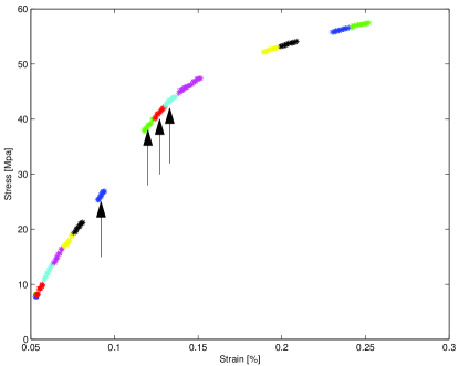
Figure 4.7: Stress-strain curve for the continuous deformation from $0\%$ (see also table 4.1). The individual markers correspond to one $\omega$-slice, and the colors indicate the strain ranges of the 3D maps. The arrows indicate the four maps illustrated in figure 4.8. The reason for the gaps (corresponding to missing datasets) is that the peak had to be re-centered due to grain rotations, and while this was done no 3D maps could be obtained.

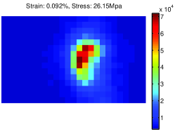
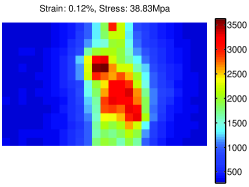
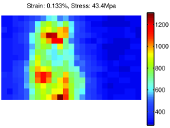
Figure 4.8: Projection onto the azimuthal plane of 3D reciprocal space maps obtained during continuous tensile deformation from $0\%$. The projections are shown as a function of stress and strain. The images span $\approx 25\cdot 10^{-3}\rAA$ horizontally (corresponding to $-\bm{q}_{x}$) and $\approx 9\cdot 10^{-3}\rAA$ vertically (corresponding to $\bm{q}_{z}$). Note that the color scales are different at the different strain levels.

4.4.2 Stability of dislocation structures

A more controlled experiment can be performed by continuous deformation of a pre-strained sample.

A grain with the tensile axis close to a $\left<100\right>$ direction was identified, and the sample was pre-strained stepwise to $1.82\%$ tensile deformation. A calibration curve for strain increment and vertical sample movement as a function of tension motor movement was found by following the grain with the X-ray beam during this initial straining. Further information in table 4.1 and newdyn.

The sample was thereafter strained continuously at different strain rates, and with different following stress relaxation times. Figure 4.9 shows the tension motor movement and the stress-strain curve for the full loading cycle, comprising two slow loadings with strain rate $1.1\cdot 10^{-6}\mathrm{s}^{-1}$, one fast loading with strain rate estimated to be $3\cdot 10^{-2}\mathrm{s}^{-1}$, and the offloading of the sample.

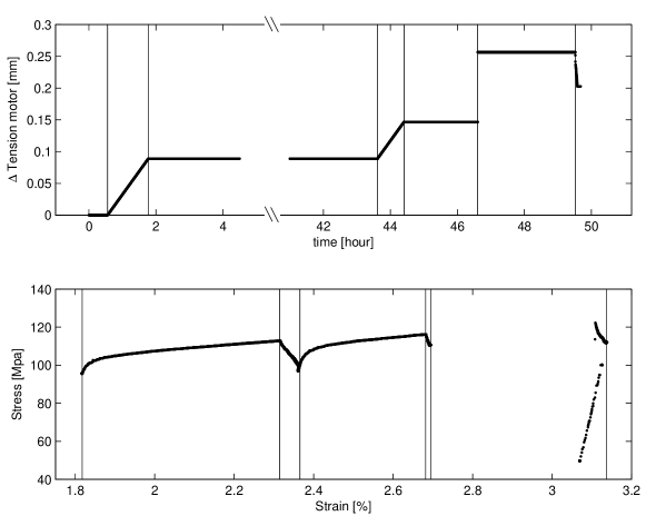
Figure 4.9: Loading cycle for the continuous deformation of a pre-strained sample. Top) Displacement of tension motor. Bottom) Stress-strain curve. Vertical lines on the two figures identify the “events” of the loading cycle. From newdyn.

Time	Strain
$-20$ minutes	$2.572\%$
$-16$ minutes	$2.593\%$
$-13$ minutes	$2.614\%$
$-9$ minutes	$2.633\%$
$-6$ minutes	$2.653\%$
$-2$ minutes	$2.672\%$
$2$ minutes	$2.683\%$
$9$ minutes	$2.685\%$
$16$ minutes	$2.686\%$
$23$ minutes	$2.687\%$
$30$ minutes	$2.688\%$

Figure 4.10: Projections onto the azimuthal plane of the last six 3D reciprocal space maps obtained during the second slow straining, and every second of the maps obtained after the straining was stopped. The time given is with respect to the time where the straining was stopped. The projections each cover $0.12\rAA$, and $0.009\rAA$ in the $q_{x}$ and $q_{z}$ directions respectively. Adapted from newdyn.

$3.137\%$, $112\mathrm{M}\mathrm{Pa}$

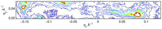
$3.069\%$, $50\mathrm{M}\mathrm{Pa}$

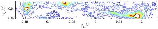
Figure 4.11: Projections onto the azimuthal plane of the 3D reciprocal space maps obtained before and after the offloading of the sample. From newdyn.

Small 3D reciprocal space maps, comprising 15 $\omega$-slices each, were obtained during the slow straining and the holding periods. Figure 4.10 shows a sequence of projections of such maps obtained during the second slow loading and holding. Larger maps were obtained before and after the offloading, projections of these maps are shown in figure 4.11. The 3D maps were also projected onto the radial direction and the integrated radial peak profiles analyzed, the resulting peak positions and widths are shown in figure 4.12.

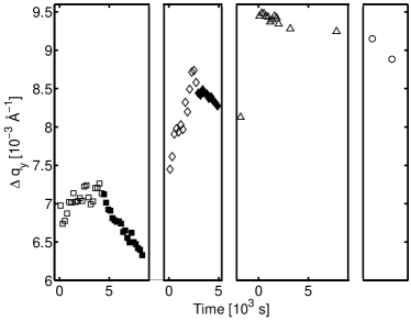
Figure 4.12: Position and width of the azimuthal integrated peak profiles as a function of time. The time is in each part measured with respect to the start of the deformation. 1. slow loading (open square), 1. holding (filled square), 2. slow loading (open diamond), 2. holding (filled diamond), fast loading (triangles pointing up), offloading (circles).

What may be observed is that the subgrain structures develop and change as long as the deformation is in progress; this is seen directly from the azimuthal projections (figure 4.10). The increase in the width of the integrated radial peak profile during the deformation, as seen on figure 4.12, indicates that the internal strain distribution broadens as the sample deforms. When the deformation is stopped the overall structure seems to freeze, and only minor changes are observed in the structures as seen from the azimuthal projections. A clear relaxation is however observed in the width and position of the radial profiles. The relaxation observed in the peak position is no surprise as this corresponds to the observed macroscopic decrease in stress.

The visual impression of the minor changes in the azimuthal projection is that the individual peaks become sharper, corresponding to some cleanup processes in the structure, which is consistent with the decrease in width of the average internal strain distribution.

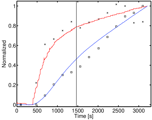
Figure 4.13: Analysis of the correlation between the macroscopic stress (red line), macroscopic strain (blue line), mean elastic strain as found from the position of the integrated peak profile ($\times$), and subgrain peak position in the $\bm{q}_{x}$-direction ($\square$). Data are taken during the second loading, after a long (41 hours) stress relaxation period. The vertical line indicates the point where the macroscopic stress reaches the previous maximum flow stress. All four curves have been normalized to give best agreement at the start and end of the deformation.

This substantiates the conclusion from the last section, that is, the dislocation structural formation and development is part of the plastic deformation process, and the structures observed after stopping the deformation are the same as the ones existing while straining. The observed stress relaxation seems (on the timescale of the experiment $\approx 1\mathrm{h}$) to be connected to a clean up process in the walls and subgrains, and not to major rearrangements of the structure.

To further investigate when the subgrain structure starts to evolve, one separated peak was selected from the data obtained during the second slow loading. This case is special, as the sample had been left for stress relaxation for $41$ hours before the measurement, the stress relaxation was therefore substantial. The peak clearly rotates (shifts) with respect to the rest of the structures observed in the maps. Figure 4.13 shows the macroscopic stress and strain, together with the position of the mean $q_{y}$-position of the integrated radial peak profile and finally the $q_{x}$-position of the selected peak. All data have been normalized to coincide at the start and end of the deformation. The time where the macroscopic stress reaches the previous maximum flow stress is furthermore indicated. What can be observed is that the position of the mean value of the radial profile follows the macroscopic stress as expected from elastic expansion. From the macroscopic stress curves it is furthermore seen that the material starts to yield before reaching the previous maximum flow stress, this must be due to the pronounced relaxation process which took place during the long holding period. The $q_{x}$-position of the peak is overall linearly dependent on the macroscopic strain, but a significant deviation from linearity is seen around the point where the macroscopic stress reaches the previous maximum flow stress.

The deviation from the linear dependence between the $q_{x}$-position of the individual peak and the macroscopic strain starts a certain amount of strain after the material has started to deform plastically, but before the previous maximum flow stress has been reached. This can be understood in the framework of the composite model, as it predicts a two stage yield process. Initially only the dislocation free subgrains will deform plastically and then later the harder walls also deform plastically. This suggests that the evolution of the subgrain structure only happens when the entire dislocation structure is deforming plastically.

Before and after the offloading of the sample larger reciprocal space maps were obtained. Projections of these are shown in figure 4.11. What can be seen is that the offloading of the sample does not give rise to changes in the overall structure (some rotation is however observed). The result is in line with a recent X-ray based experiment by Schafler2005, who report in-situ synchrotron-based line broadening studies of $[100]$ orientated single crystals. At selected strains Schafler and co-workers interrupted the deformation, unloaded the crystal, reloaded and continued the deformation [Ungar2006Pers]. Peak profiles were obtained at all stages, and no differences existed between the average dislocation density during loading, under load, and in the offloaded state [Ungar2006Pers].

Beside the investigation of the overall structural changes due to offloading seven individual peaks were analyzed using the single peak analysis methods presented in section 3.6.3. The peaks clearly move in the azimuthal directions during the offloading. The analysis shows that the movement is mainly due to elastic rotation of the full structure (average shifts of $-0.0072\rAA$ and $-0.0024\rAA$ were found in the $\bm{q}_{x}$- and $\bm{q}_{z}$-direction respectively). However a significant spread was observed in the individual rotations, the standard derivations being $13\%$ and $20\%$ of the average rotation in the $\bm{q}_{x}$ and $\bm{q}_{z}$ directions respectively.

The $\bm{q}_{y}$-positions of the individual peaks showed that a backwards strain (as discussed in section 4.2) also exists in this case. What may be observed is that the magnitude of the mean backwards strain increased by $14\%$ upon the offloading. This is consistent with the results presented in [borbely00], which are based on traditional line profile analysis on Cu single crystals deformed under constant load. More interestingly the width of the distribution of strains between the subgrains decreased by the significant amount of $31\%$.

This shows that the general structure is independent of offloading. However, offloading does change the internal strain distribution and the exact orientation differences between the subgrains.

4.5 Subgrain refinement

A prominent feature of the dynamics of a dislocation structure is the cell refinement process, that is the fact that the average size of the subgrains goes down as the plastic deformation increases.

Traditionally this refinement is attributed to the trapping of dislocations inside subgrains, which leads to the buildup of new boundaries with corresponding orientation differences between the two sides (e.g. [Hughes1997a]). The signature of such a process would be that the peak from the initial subgrain started to broaden, as dislocations get trapped, and then divided into two peaks rotating away from each other.

It is possible to follow such a process by mapping the same region in reciprocal space as a function of strain. The results and experimental details are also reported in science.

A grain, having the tensile axis close to a $\left<100\right>$ orientation, was identified. The sample was pre-strained to $3\%$ elongation and then from $3\%$ to $4.2\%$ in steps of $\approx 0.04\%$ while following the grain. The beam used was reduced to $14\mathrm{\SIUnitSymbolMicro}\mathrm{m}\times 14\mathrm{\SIUnitSymbolMicro}\mathrm{m}$ by slits. The illuminated part of the grain was kept constant with respect to the center of the grain by spatial scanning of the grain at (almost) all strain steps. This scanning procedure has the consequence that possible beam drift problems (as described in section 3.2.1) are corrected for.

Figure 4.14 shows a projection onto the azimuthal plane for one of the 3D reciprocal space maps obtained. By keeping the stain increments small and the maps relatively large (in the $\bm{q}_{z}$-direction), it is ensured that the possible rotation of the individual subgrains can be followed in detail. By making movies, consisting of projections onto the azimuthal plane as a function of strain, it is verified that the individual peaks can be followed (one such movie is published as “Supporting Online Material” in connection with science).

An increase in strain from $3\%$ to $4.2\%$ corresponds to an increase in the number of subgrains of $\approx 66\%$ assuming an inverse square root law of the boundary spacing as a function of strain [Hughes1997a]. By this is should be highly likely to observe the signature of subgrain refinement, as more than half the subgrains have to be “refined”.

Approximately $20$ peaks were followed for some strain intervals, and in no cases were a clear signature of a subgrain breakup observed. However, we did observe an unexpected intermittent dynamics, peaks appearing out of regions of enhanced intensity, exist for some strain steps before they disappear again. Figure 4.15 shows an example of such an event. Our interpretation of this is, that the subgrains “materialize” out of regions of high dislocation density, stay for some time and then “dissolve” again.

The picture of intermittent dynamics constitutes an alternative framework for understanding the dynamics of dislocation structures. It may e.g. explain how a preferred orientation of dislocation boundaries are kept during cold working.

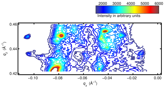
Figure 4.14: Projection on to the azimuthal plane of a 3D reciprocal space map obtained at $3.49\%$ tensile strain from the stepwise deformation experiment. From science.

Figure 4.15: Excerpts form larger azimuthal projections of reciprocal space maps taken at stepwise increasing strain. These are shown from left to right as a function of external strain. Strain increments are relative to the first map shown. Example of a peak appearing, existing for some strain interval (note the $\cdots$ indicting that multiple strain steps where the peak was visible, have been left out), and then disappearing. Color scale and contour lines identical as in figure 4.14. Adapted from science.

Chapter 5 Conclusions and outlook

The main aim of this study has been in-situ investigations of bulk deformation structures in simple polycrystalline fcc metals at low degrees of deformation. Both the dynamics of such structures during deformation and the static properties under load have been investigated.

The outcome has been two fold; a novel technique has been established and a number of fundamental scientific questions have been addressed.

The technique

The novel synchrotron radiation-based technique “High Angular Resolution 3DXRD”, which has been developed, extends the 3DXRD microscopy technique to high resolution 3D reciprocal space mapping. The technique has a number of advantages over traditional 3D reciprocal space mapping techniques:

• Individual broadened reflections from deeply embedded single grains in a polycrystalline sample can be mapped, due to the high energy ($52\mathrm{k}\mathrm{eV}$).

• The mapping is relatively fast due to the high flux and the fact that only one degree of freedom has to be swept to obtain a 3D map. The typical acquisition time for one $\omega$-slice is $10\mathrm{s}$. This enables in-situ experiments during deformation, as a stress rig has been incorporated in the setup.

• The voxels in reciprocal space, mapped onto one data point, are close to being cube-shaped, giving an equivalent resolution in all directions. The dimensions of the voxels are $\approx 1\cdot 10^{-3}\rAA$ in the radial and in one azimuthal direction, if defined by the instrumental broadening. The dimension in the perpendicular azimuthal direction is defined by the rocking angle interval.

The resolution of the technique corresponds to a strain resolution of $0.7\cdot 10^{-4}$ or better. This is as good as or better than other existing techniques for measuring the strain in individual subgrains.

The orientation resolution is $\approx 0.007\mathrm{\SIUnitSymbolDegree}$, which is an order of magnitude better than TEM-based methods.

Interpretation of 3D reciprocal space maps from cell-forming metals

The technique has been used to investigate polycrystalline copper at low degrees of plastic tensile deformation ($<5\%$ strain).

It was found that the broadened reflections, from such a cell-forming metal, comprise a structure consisting of bright sharp peaks (separable in 3D in the reciprocal space) superimposed on a cloud of enhanced intensity. Based on the size of the scattering entities, the width of the peaks and spatial separation it is concluded that the peaks arise from individual subgrains (dislocation-free regions) deeply embedded in the grain investigated. The cloud is inferred to arise from the dislocation-filled walls in the dislocation structure.

The technique developed provides a unique direct probe of the properties of individual subgrains in bulk grains, something which has been unavailable previously. A number of scientific issues regarding the dislocation structure have been investigated using this technique.

Static results

Based on static investigations of grains, with the tensile axis close to a $\left<100\right>$ orientation, in deformed samples under load it is found that:

• The subgrains on average are subjected to a reduction of the elastic strain, compared to the mean strain of the full grain, when lattice planes perpendicular to the tensile axis are investigated (the axial case). The size of this strain reduction is on the order of $10$–$25\%$ of the average elastic strain in the grain. An increase in the elastic strain is by contrast observed from the lattice planes parallel to the tensile axis, and the ratio of these two “internal” strains is close to the Possion ratio.

• Evidence imply that the walls in the dislocation structure are subjected to an increase in elastic strain.

• The distribution of elastic strains between the subgrains is broader than the distribution of elastic strains within the individual subgrains.

• The redundant dislocation density in the subgrains is very low ($<12\cdot 10^{12}\mathrm{m}^{-2}$).

• Calculations show that as few as one excess dislocation in a subgrain might give a visible splitting of the associated diffraction peak. Such transient splittings have been observed during stepwise loading.

The observed elastic strain distribution suggest that the composite model by Mughrabi correctly describes the elastic strain distribution on average, but that asymmetric peak profile analysis has to be reinterpreted.

Dynamic results

A number of in-situ experiments have been performed, investigating the properties of the dislocation structure during and after deformation.

The development of the dislocation structure was followed during continuous deformation from the undeformed state. The subgrains clearly form during the deformation, and seemed to start forming as soon as plastic deformation is detectable (in one case investigated at around $0.12\%$ elongation). Additionally a pre-deformed sample was continuously deformed, monitoring the subgrain dynamics during the deformation and immediately after termination of the deformation. The evolution of the dislocation structure clearly happened during the deformation, and no changes were observed at the termination point.

The consequences of $\approx 1\mathrm{h}$ stress relaxation after continuous deformation and of unloading of the sample were also analyzed. It was found that the overall dislocation structure only depends on the maximum applied stress, as no overall changes were observed in the subgrain structure during the relaxation (at least on this time scale), or after the offload. However, a minor relaxation in the width of the internal strain distribution is observed from the width of the integrated radial peak profile. On the level of the individual subgrains, it was observed that the width of the stain distribution between the subgrains decreases by a substantial amount ($31\%$ in the case investigated) and that the level of backwards strain increases slightly ($\approx 14\%$ in the case investigated) during the offloading.

Based on stepwise loading of a pre-strained sample it is found that the dislocation structure shows “intermittent” dynamics. The subgrains seem to arise out of regions with an enhanced dislocation density, exist for some time with proceeding deformation, and then eventually disappear. In none of the investigated cases was a simple subgrain breakup observed. The subgrain refinement process hens does seem to be due to this intermittent dynamics.

The results of the dynamical experiments points to a dislocation structure which is very dynamic. The structure seems to adjust itself to fit with the present environment by creating and dissolving subgrains. Furthermore, it seems that major changes happen only when the entire dislocation structure undergoes plastic deformation.

In conclusion it is my belief that measurements of this kind provide very valuable information on a scale and under conditions previously unattainable. Hopefully, the results can inspire a new generation of work hardening and pattern formation models.

Outlook

The results presented in this thesis have shown that High Angular Resolution 3DXRD is a very promising technique for investigating subgrains and their dynamics.

One of the most surprising results is the observation of intermittent dynamics. However subgrain refinement experiments at higher strains are needed to show if these findings are general for plastic deformation or only apply at the early stages of the pattern formation (see e.g. comment by Kubin2006).

Furthermore a number of additional scientific cases, which are in line with the present study, are candidates for being studied by High Angular Resolution 3DXRD:

Strain path change.

As the deformation structure depends on the mode of deformation, it will need to adapt itself if the strain path is changed. It would be very interesting, and possible, to investigate if the structure gradually changes from one to another by e.g. rotation of subgrains, or if the change is mediated through a process of “dissolving-and-generation” as with the case of intermittent dynamics observed in unidirectional deformation.

Grain orientation dependence of internal strain.

The grains investigated in this thesis all have an orientation which results in a cell-like morphology of the dislocation structure. The possible grain orientation dependency of the internal strain distribution can be studied by investigating grains of different orientations, and mapping multiple reflections from each grain (as was done with low resolution in [pantleon04]). Such experiments can e.g. show if the observed forward and backwards strains also exists in grain with the more general cell-block structure.

Investigations of highly deformed materials.

The investigation of highly deformed metals is a region of material science which is attracting a lot of attention presently. We have performed proof of concept experiments on thin films and one $\omega$-slice from such a measurement is shown in figure 5.1. It is seen that it is possible to observe individual spots from the subgrains from such a highly deformed sample. Hence it should be possible to investigate e.g. internal strain differences in such materials.

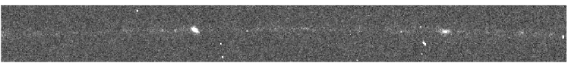
Figure 5.1: A single $\omega$-slice (covering $0.01\mathrm{\SIUnitSymbolDegree}$) taken on the 220 ring from a thin film of highly deformed aluminum. Two clear peaks are seen on a rather smooth background. The degree of deformation is unfortunately unknown but very high (von Mises strain $>5$). This is from the very first experiment, therefore the 3DXRD peak shape analysis setup was used (see section 2.5.3).

To be able to fully perform such experiments a few experimental developments are needed, to improve the statistics and stability of the measurements:

Automated peak finder for 3D reciprocal space maps.

The individual peaks are presently located manually from azimuthal projections of 3D maps. This is rather time consuming, and it is not feasible to investigate all peaks in a large map. An automated procedure would give better statistics, and a more unbiased peak selection.

Full 3D fitting of peaks.

The individual peaks are presently analyzed by fitting line profiles through the peak, the full 3D information is therefore not used in the analysis. An automated 3D fitting routine should be able to give better information on the integrated intensity, and the true shape of the peak. Furthermore 3D multi peak fitting may allow for better separation of partially overlapping peaks, and hence give access to more peaks.

Beam position monitor and feedback systems for improved stability.

The major experimental problem is presently the instability of the beam position. This has the consequence that the relative intensity between peaks might change over time, due to beam drift, which can only be partly corrected for by tedious spatial scanning of a grain with respect to the beam. A feedback system should be able to keep the position of the beam constant, and thereby the intensity profile on the sample constant.

Even higher resolution and/or better characterization of the instrumental resolution.

The instrumental broadening contributes significantly to the width and shape of the individual peaks from the subgrains. If precise measurements of internal strain distribution or dislocation density in the individual subgrains are wished for, it is important to be able to fully separate the contribution from the instrument and the real physical peak profile. This could be obtained in two ways; firstly if the instrumental broadening could be characterized better, a deconvolution could be performed, secondly the instrumental broadening could be reduced so much that its contribution is negligible. The major problem with characterizing the instrument is that it is hard to find a probe which can be used for the measurement. If small grains in a powder are used, size broadening will influence the measurement, and if a perfect single-crystal is used, full dynamical scattering theory is needed. Reduction of the instrumental broadening is not easy either as all contributions are of the same order of magnitude, hence major parts of the setup would have to be improved to give a significant improvement. However, a detector with a smaller point spread would improve on this (a reduction by a factor of 2 in the point spread would give a reduction of the theoretical experimental broadening by $20\%$). It should be mentioned that the Darwin width of a Cu 400 reflection is $\approx 3\cdot 10^{-4}\rAA$ only a factor $3$ – $4$ away from the present resolution.

One important observation is the diversity of the 3D shapes of the peaks from the individual subgrains, which varies from flat disks through spheres to needle shapes. This must be because of differences in dislocation configurations and boundary conditions. In section 4.3 results using traditional line profile analysis and simple atomistic calculations were presented. It should be possible to obtain more information from the 3D shape of the peaks.

A possibility might be to make full 3D simulations of subgrains with embedded dislocations and given boundary conditions. Such simulations could give an insight into how dislocation configuration and density influence the shape of the 3D diffraction peak. Ultimately it might be possible to make a fitting routine which matches the calculated peak to the measured 3D peak using the dislocation configuration as the “fitting parameter”.

Finally I emphasize that, High Angular Resolution 3DXRD as such is not limited to investigations of dislocation structures and their dynamics under deformation. Examples of other applications are:

General elastic strain distributions.

An equivalent investigation on strain distributions to the one presented in section 4.2 can be performed on any sample which consists of a number of incoherently scattering entities (e.g. crystallites in a powder). By 3D reciprocal space mapping it will be possible to investigate if each entity has an internal strain distribution or if the strain is mainly distributed between them (a previous example of such results exists in [Fewster1999] on the grain scale in a polycrystalline sample). Such investigations could be of major importance for interpretation of e.g. powder diffraction signals.

Peak separation.

A general condition for 3DXRD experiments is that a separation of individual diffraction peaks is needed. High Angular Resolution 3DXRD might be a possible route for separating reflections which overlap when observed by the (relatively) low angular resolution of the normal 3DXRD microscope.

Annealing experiments.

Annealing phenomena in the deformation structure can be investigated by including a furnace in the setup. This could e.g. be for investigations of the recovery process of highly deformed samples. Such experiments would benefit from the ability to separate individual peaks, and would allow for investigating not only the volume and orientation (as in [Gundlach2004] where traditional 3DXRD is used for such experiments) but also allow for monitoring the internal strain distribution as a function of time.

Bibliography

My publications

mypubl

Cited publications

../bibfiler/metal,../bibfiler/OurPublications