Constraining the nature of High Frequency Peakers

Abstract

Aims. We investigate the spectral characteristics of 51 candidate High Frequency Peakers (HFPs), from the “bright” HFP sample, in order to determine the nature of each object, and to obtain a smaller sample of genuine young radio sources.

Methods. Simultaneous multi-frequency VLA observations carried out at various epochs have been used to detect flux density and spectral shape variability in order to pinpoint contaminant objects, since young radio sources are not expected to be significantly variable on such a short time-scale.

Results. From the analysis of the spectral variability we find 13 contaminant objects, 11 quasars, 1 BL Lac, and 1 unidentified object, which we have rejected from the sample of candidate young radio sources. The $\sim$6 years elapsed between the first and latest observing run are not enough to detect any substantial evolution of the overall spectrum of genuine, non variable, young radio sources. If we also consider the pc-scale information, we find that the total radio spectrum we observe is the result of the superposition of the spectra of different regions (lobes, hot-spots, core, jets), instead of a single homogeneous radio component. This indicates that the radio source structure plays a relevant role in determining the spectral shape also in the rather common case in which the morphology appears unresolved even on high-resolution scales.

1 Introduction

The origin and evolution of radio emission is one of the greatest challenges in the study of Active Galactic Nuclei. The onset of radio activity is often thought to be linked to merger or accretion events in the host galaxy, which provide enough fuel to feed the central AGN. As a consequence, at least in its early stages, the radio emission evolves in a quite dense and possibly inhomogeneous ambient medium which can influence its growth.
The ideal targets to understand such phenomena are the young radio sources, whose radio lobes still reside within the innermost region of the host galaxy.
Among them, the smallest (i.e. youngest) objects are the most suitable to investigate the role played by the host galaxy Interstellar Medium (ISM) on the evolution/growth of the radio source.
The evolutionary stage of the powerful radio sources is related to their linear sizes. Following self-similar evolution models, the most compact sources will evolve into the extended radio source population (Fanti et al. cf95 (1995); Readhead et al. rh96 (1996); Snellen et al. sn00 (2000)).
However, it has also been claimed (Alexander alexander00 (2000); Marecki et al. ma03 (2003)) that a fraction of young and compact radio sources may die in an early stage before becoming large scale objects.
The early stages in the evolution scheme (typical ages $<$ 10⁴ years, Polatidis & Conway pc03 (2003); Murgia mm03 (2003)) are represented by the population of Compact Symmetric Objects (CSOs). They are a scaled-down version of the large, powerful radio sources (core-jets-lobes; Wilkinson et al. wil94 (1994)), with a well defined peak in their radio spectrum at frequencies between $\sim$ 100 MHz to a few GHz.
In this framework, the anti-correlation found between the intrinsic peak frequency and the source size (O’Dea & Baum odea97 (1997)) implies that the youngest sources must be sought among those with spectral peaks occurring at frequencies higher than 5 GHz, and termed “High Frequency Peakers” (HFPs, Dallacasa dd03 (2003)).
The selection of a statistically complete sample made of genuine young radio sources only is essential to study in detail the physical nature of this class of objects.
A sample of candidate HFPs (the “bright” sample; Dallacasa et al. dd00 (2000)) was constructed on the basis of both the shape of the simultaneous radio spectrum and the turnover frequency. However, such selection tools can introduce a contamination by beamed radio sources. For example, blazar objects, although usually characterized by a flat spectrum, can occasionally show a convex spectrum when their radio emission is dominated by a flaring, self-absorbed component (e.g. Torniainen et al. torni05 (2005)).
During the majority of their lifetime blazars and young radio sources display very different characteristics: the former posses significant flux-density and spectral variability, and the emission, often polarized, has a Core-Jet morphology on various scales (from tens of kpc down to pc-scale). The latter have no variability and the radio emission, almost completely unpolarized at least at low frequencies, has a “Double/Triple” structure (Orienti et al. mo06 (2006)).
In this paper we present the results of simultaneous multi-frequency VLA observations, made at several epochs, in addition to those already published by Dallacasa et al. (dd00 (2000)) and Tinti et al. (st05 (2005)). These new observations were carried out to further identify blazars with variability on time-scales longer than the time elapsed between the previous two epochs (Tinti et al. st05 (2005)), and to study the evolution of the radio spectrum of those HFPs already confirmed as genuine young radio sources (Orienti et al. mo06 (2006)).
In general, they better characterize the properties of the sources of the “bright” HFP sample.

Date	Conf	Obs Time	code
Sep 12 2003	AnB	240	a
Sep 13 2003	AnB	240	b
Sep 14 2003	AnB	240	c
Sep 15 2003	AnB	620	d
Jan 22 2004	BnC	120	e
Jan 26 2004	BnC	180	f
Jan 28 2004	BnC	240	g
Jan 30 2004	BnC	120	h
Mar 21 2004	CnD	120	i

Table 1: VLA observations and configurations. The total observing time (Column 3) is inclusive of the scans on the HFPs from the “faint” sample.

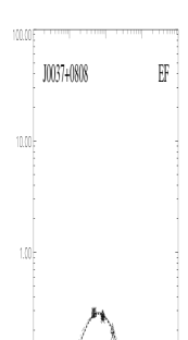
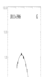
Figure 1: Radio spectra of the 51 candidate HFPs observed with the VLA during the observing runs presented in this paper [$S_{\nu}$ (Jy) vs $\nu$ (GHz)]: crosses, plus signs and diamonds refer to the first (1998-1999; Dallacasa et al. dd00 (2000)), second (2002; Tinti et al. st05 (2005)), and our third epoch (2003-2004; dates are reported in Table 1) of simultaneous VLA observations, while the dashed alternated by three dots, the dotted and the solid lines indicate the corresponding fits. When a fourth epoch was available (2004; dates are reported in Table 1), it is represented by triangles and a dash-dot line.

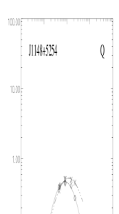
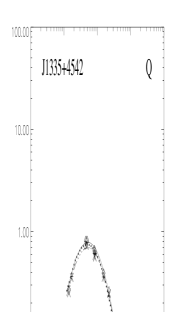
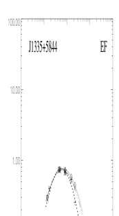
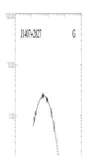
Figure 1: Continued.

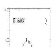
Figure 1: Continued.

2 Multi-frequency VLA observations and data reduction

Multi-frequency VLA observations of 51 of the 55 candidate HFPs were carried out in different runs from September 2003 to March 2004, using filler time. About 25 objects were observed twice, in order to identify short-period variability.
The observing bandwidth was chosen to be 50 MHz per IF. Separate analysis for each IF in L, C and X bands was carried out to improve the spectral coverage of the data, as done in previous works (Dallacasa et al. dd00 (2000); Tinti et al. st05 (2005)).
We obtained the flux density measurements in L band (IFs at 1.465 and 1.665 GHz), C band (4.565 and 4.935 GHz), X band (8.085 and 8.465 GHz), U band (14.940 GHz), K band (22.460 GHz), and for a few datasets in Q band (43.340 GHz).
Each source was typically observed for 50 seconds at each band, cycling through frequencies. Therefore, the flux density measurements can be considered simultaneous.
For each observing run and at each frequency, about 3 min were spent on the primary flux density calibrator, either 3C 286 or 3C 48. Secondary calibrators, chosen to minimize the telescope slewing time, were observed for 1.5 min at each frequency every $\sim$20 min. This implies that the observations do not have astrometric accuracy. Accurate positions of the sources can be found in the JVAS catalogue (Patnaik et al. patn92 (1992); Browne et al. browne98 (1998); Wilkinson et al. wil98 (1998)). Information on the date and duration of the observing runs is summarized in Table 1. The total observing time also takes into account scans on candidate HFPs from the “faint” HFP sample (Stanghellini et al., in preparation), in order to optimize the observing schedule.
The data reduction was carried out following the standard procedures for the VLA, implemented in the NRAO AIPS package. Images for each frequency were produced. In order to obtain accurate flux density measurements in the L band, it was necessary to image several confusing sources falling within the primary beam, and often accounting for most of the flux density within the field of view.
During some observing runs, strong RFI affected the 1.665 GHz data, precluding the flux density measurements for a few sources at such frequency.
The final images were produced after a few phase-only self-calibration iterations, and source parameters were measured by means of the task JMFIT, which performs a Gaussian fit. The integrated flux density was checked with TVSTAT. The flux density measurements at each frequency and epoch are reported in Table 2.
Apart from a few sources that were already known to possess an extended emission (Tinti et al. st05 (2005)), the majority of HFPs are unresolved with the VLA, even in the Q band.
The r.m.s. noise level on the image plane is not relevant for bright radio sources as our targets. In this case, the main uncertainty comes from the amplitude calibration errors, which is within (1$\sigma$) 3% in L, C and X band, 5% in U band, and 10% in K and Q band.
With these new-multi-frequency observing runs, 48 out of the 55 sources from the bright HFP sample have at least three epochs of VLA data. The comparison between each epoch allows us to determine the variability properties of each single source.

3 Results

The lack of any spectral variability is a key element for the selection of genuine young radio sources. The new epochs of simultaneous multi-frequency VLA observations, carried out 5-6 years after the first observing run (Dallacasa et al. dd00 (2000)), provide further information on the spectral shape and variability of the candidate HFPs, allowing us to better discriminate between genuine young radio sources and contaminant objects.

Source	Id.	z	code	S1.4	S1.7	S4.5	S4.9	S8.1	S8.4	S15.3	S22.2	S43.2	$\alpha_{\rm below}$	$\alpha_{\rm above}$
(1)	(2)	(3)	(4)	(5)	(6)	(7)	(8)	(9)	(10)	(11)	(12)	(13)	(14)	(15)
J0003+2129	G	0.455	d	100	125	258	262	233	227	146	70	-	-0.8	0.9
			e	84	-	251	255	226	220	134	70	16	-0.9	1.3
J0005+0524	Q	1.887	c	166	174	212	206	169	165	122	84	-	-	0.6
			e	168	-	213	207	170	168	129	90	46	-	0.6
J0037+0808	G		c	98	119	287	290	273	267	197	139	-	-0.9	0.5
			e	95	-	287	293	278	274	210	148	79	-0.9	0.6
J0111+3906	G	0.668	c	509	597	1319	1301	965	918	449	273	111	-0.8	1.1
J0116+2422	EF		c	106	122	245	244	240	226	177	121	-	-0.7	0.4
			e	99	-	258	238	240	225	177	129	-	-	0.4
J0217+0144	Q	1.715	c	577	514	337	326	268	263	244	239	-	-	0.3
			e	571	-	326	315	257	264	256	254	-	-	0.3
J0329+3510	Q	0.5	d	410	443	603	611	586	578	523	447	-	-0.3	0.2
			g	563	-	644	625	540	535	468	401	302	-	0.2
J0357+2319	Q		d	116	124	242	255	309	312	382	373	-	-0.5	-
			g	-	-	185	187	208	210	239	232	212	-0.2	0.1
J0428+3259	G	0.479	d	148	195	513	524	539	531	421	269	-	-0.8	0.6
			g	172	199	497	512	522	520	394	253	104	-0.7	0.9
J0519+0848	EF		c	269	263	394	393	373	372	365	336	-	-0.4	0.1
			g	262	273	314	320	322	321	372	382	348	-0.1	0.1
J0625+4440	BL		c	173	186	223	222	219	218	197	174	-	-0.2	0.1
			g	121	131	180	182	187	187	180	161	121	-0.2	0.2
J0638+5933	EF		c	249	315	605	619	680	678	701	653	-	-0.5	-
			g	300	325	597	608	649	651	706	643	412	-0.4	0.5
J0642+6758	Q	3.180	c	226	272	436	429	343	332	205	131	-	-0.5	0.7
			g	190	238	405	402	320	312	204	123	44	-0.6	0.9
J0646+4451	Q	3.396	c	444	660	2860	3071	4068	4124	3944	3184	-	-1.3	0.3
			g	586	717	2894	3103	4064	4094	4039	3175	1996	-1.1	0.5
J0650+6001	Q	0.455	c	507	633	1161	1150	994	975	674	467	-	-0.7	0.5
			g	480	626	1150	1106	958	935	798	466	204	-0.7	0.7
J0655+4100	G	0.02156	c	209	232	323	330	354	354	319	268	-	-0.3	0.3
			g	198	233	351	341	369	369	360	307	226	-0.3	0.3
J0722+3722	Q	1.63	d	148	180	199	199	178	174	138	99	-	-	0.4
			g	171	188	203	203	176	172	125	83	44	-	0.7
J0927+3902	Q	0.6948	d	2810	3615	9545	9760	10027	9937	8813	7237	-	-0.8	0.3
J1016+0513	Q		d	633	711	489	478	428	420	388	327	-	-	0.3
J1045+0624	Q	1.507	d	185	245	296	289	268	266	226	152	-	-	0.4
J1148+5254	Q	1.632	a	108	-	396	414	460	450	411	277	-	-0.9	0.4
J1335+4542	Q	2.449	a	267	-	821	821	666	646	392	263	-	-0.9	0.7
J1335+5844	EF		a	299	-	745	744	727	726	585	449	-	-0.8	0.3
J1407+2827	G	0.0769	b	865	1133	2519	2532	2147	2071	1027	542	-	-0.8	1.0
J1412+1334	EF		b	191	248	346	341	286	277	189	121	-	-0.5	0.6
J1424+2256	Q	3.626	b	371	480	652	637	-	394	247	144	-	-0.4	0.9
J1430+1043	Q	1.710	b	321	423	865	861	780	767	582	473	-	-0.8	0.4
J1505+0326	Q	0.411	b	382	428	608	620	620	610	515	468	-	-0.3	0.2
J1511+0518	G	0.084	b	92	123	569	608	801	811	763	573	-	-1.3	0.3
J1526+6650	Q	3.02	d	109	-	426	440	380	369	211	104	-	-1.1	1.0
J1623+6624	G	0.203	d	154	-	282	281	257	254	191	123	-	-0.5	0.5
			i	162	179	265	263	227	221	164	122	80	-0.4	0.5
J1645+6330	Q	2.379	d	280	-	419	430	464	463	410	273	-	-0.3	0.5
			i	270	288	391	399	430	432	401	322	192	-0.3	0.5
J1717+1917	Q	1.81	h	211	211	232	232	210	208	174	144	124	-0.1	0.3
J1735+5049	G		h	445	-	925	943	898	888	678	485	262	-0.6	0.6
			i	436	479	935	945	886	873	623	408	140	-0.6	0.9
J1751+0939	BL	0.322	h	980	1120	2714	2848	3825	3897	4556	4583	4642	-0.5	-
J1800+3848	Q	2.092	f	262	326	793	836	1109	1128	1249	1147	758	-0.7	0.5

Table 2: The VLA flux density of the 51 candidates HFPs observed with the VLA during the observing runs presented in this paper. Col. 1: source name (J2000); Col. 2: optical identification; Col. 3: redshift; Col. 4: the observation code, from Table 1; Col. 5, 6, 7, 8, 9, 10, 11, 12, and 13: VLA flux density in mJy at 1.4, 1.7, 4.5, 4.9, 8.1, 8.4, 15.3, 22.2 and 43.2 GHz respectively; Col. 14: spectral index below the peak frequency; Col. 15: spectral index above the peak frequency.

Source	Id.	z	code	S1.4	S1.7	S4.5	S4.9	S8.1	S8.4	S15.3	S22.2	S43.2	$\alpha_{\rm below}$	$\alpha_{\rm above}$
(1)	(2)	(3)	(4)	(5)	(6)	(7)	(8)	(9)	(10)	(11)	(12)	(13)	(14)	(15)
J1840+3900	Q	3.095	f	123	147	161	163	165	165	165	164	140	-0.1	0.1
J1850+2825	Q	2.560	f	235	280	1097	1185	1515	1520	1402	1132	605	-1.1	0.6
J1855+3742	G		f	180	181	360	344	215	206	123	86	50	-0.6	0.9
J2021+0515	Q		f	360	442	520	506	407	397	285	206	100	-0.3	0.7
J2024+1718	Q	1.05	f	307	324	594	609	623	619	519	403	242	-0.5	0.6
J2101+0341	Q	1.013	c	483	493	497	498	552	555	704	724	-	-0.2	-
			f	431	-	498	508	665	687	954	1031	883	-0.3	0.2
J2114+2832	Q	2.345	d	414	493	612	599	545	535	458	357	-	-0.3	0.3
J2123+0535	Q	1.878	f	2185	2260	2831	2879	3054	3057	3021	2740	1992	-0.1	0.2
J2136+0041	Q	1.932	c	4234	5231	10284	10225	8763	8601	6252	4401	-	-0.7	0.5
			f	3752	4823	10193	10150	8779	8599	6343	4720	2578	-0.8	0.6
J2203+1007	G		c	107	156	315	311	240	231	125	67	21	-0.9	1.2
J2207+1652	Q	1.64	d	177	206	220	224	227	226	214	177	-	-0.1	0.2
			e	268	-	242	248	246	246	218	183	151	-	0.2
J2212+2355	Q	1.125	d	490	576	659	651	629	625	631	547	-	-0.2	0.1
			e	507	-	634	644	682	684	695	624	517	-0.1	0.3
J2257+0243	Q	2.081	c	199	199	280	295	400	408	480	426	-	-0.4	0.3
			e	180	-	291	306	420	432	517	466	330	-0.5	0.5
J2320+0513	Q	0.622	c	526	541	968	1006	1144	1148	1114	936	-	-0.5	0.2
			e	615	-	1060	1076	1098	1094	996	844	616	-0.4	0.3
J2330+3348	Q	1.809	d	274	-	498	511	596	603	620	525	-	-0.3	0.4

Table 2: Continued

3.1 Spectral shape

The shape of the radio spectrum is one of the key identifying characteristics of young radio sources. The overall shape of their radio spectra is convex with a peak at high frequencies that is likely due to synchrotron self-absorption within the small radio emitting region (Snellen et al. sn00 (2000)), although free-free absorption (Bicknell et al. bick97 (1997); Kameno et al. ka00 (2000)) may play a role.
On the other hand, blazar objects, which usually show flat spectra, sometimes can display a convex spectrum as a consequence of an increment of the flux density, when a single, homogeneous and boosted component at the jet base temporarily dominates the radio emission. As the component adiabatically expands, the flux density decreases, leading the spectrum back to a flat shape.
Following the approach from Dallacasa et al. (dd00 (2000)) and Tinti et al. (st05 (2005)), we fit the simultaneous radio spectra with a function that provides the flux density and the frequency of the spectral peak, but without any physical content. Since most of the sources are optically thin at 43 GHz, the new flux density measurements at such frequency, which was not available in the previous epochs, provide very tight constraints on the fits and a better determination of the peak.
In Fig. 1, we show the radio spectra of all the sources observed at the various epochs.
Following the approach by Torniainen et al. (torni05 (2005)) we compute the spectral indices $\alpha_{\rm below}$ and $\alpha_{\rm above}$ of the overall spectrum (Col. 14 and 15 of Table 2) fitting a straight line to the parts below and above the spectral peak respectively. We consider “flat” those sources with both $\alpha_{\rm below}>-0.5$ and $\alpha<0.5$ (where $S\propto\nu^{-\alpha}$). In a few sources, depending on the peak frequency, we could fit either $\alpha_{\rm below}$ or $\alpha_{above}$, in order to avoid the flattening near the spectral peak. In this case, sources with the spectral index in the range of -0.5 and 0.5 are considered flat-spectrum objects. We find that 18 objects, labeled with an “F” in Column 9 of Table 3, no longer show the convex spectrum. Such sources are labelled “flat” in Column 5 and 6 of Table 3, and are definitely classified as “blazar”, and removed from the sample of genuine young radio sources. Six of these sources (J0217+0144, J0329+3510, J0357+2319, J2123+0535, J2320+0513 and J2330+3348) were already found with a flat spectrum in the second epoch observations, and already rejected from the sample of candidate HFPs (Tinti et al. st05 (2005)).

3.2 Variability index

As already mentioned in Section 3.1, given the large Doppler factors characterizing the blazar jets, the flux density variability can substantially modify the observed spectrum of blazars on short timescales.
On the contrary, young radio sources should not display any significant flux density variability and they can be considered as the least variable class of extragalactic radio sources (O’Dea odea98 (1998)), with a mean variation of $\sim$ 5% (Stanghellini et al. cs05 (2005)). Therefore, genuine young HFP objects, considered to be newly born radio sources, should not display significant variability.
We analyze the variability of the sources in terms of the quantity:

$$V=\frac{1}{m}\sum_{i=1}^{m}\frac{(S_{i}-\overline{S}_{i})^{2}}{\sigma^{2}_{i}}$$ (1)

which is a multi-epoch generalization of the variability index defined by Tinti et al. (st05 (2005)). S_i is the flux density at the i-th frequency measured at one epoch, while $\overline{S}_{i}$ is the mean value computed averaging the flux density at the i-th frequency measured at all the available epochs; $\sigma_{i}$ is the error on S_i $-$ $\overline{S}_{i}$, and $m$ is the number of sampled frequencies.
Columns 7 and 8 of Table 3 report the variability between each new epoch and the mean value obtained by averaging all the available epochs. The variability index V has been computed for each single new epoch, rather than considering all the epochs together. In this case the availability of two distinct values better indicates the presence of flux-density bursts.
Comparing the variability distributions computed from Eq. 1 for all the sources of each epoch, the KS test does not detect any significant difference ($>$99%). This means that the flux density of the majority of the observed sources has not changed its behaviour with time.
From the comparison of the multi-epoch radio spectra we find:

• 18 sources with a convex spectrum at the first epoch (Dallacasa et al. dd00 (2000)) show a flat spectrum in at least one of the subsequent epochs. They have an “F” in Column 9 of Table 3 and they are rejected from the sample;

• Of the aforementioned sources the quasar J2320+0513 shows a continuous alternation between a flaring-phase with a convex-shape spectrum, and a quiescent-phase where the spectrum is flat. In particular, during the second-epoch observations, the source was characterized by a flat spectrum, while during our last observing run its spectrum becomes convex again and with almost the same flux density as the first epoch. This example points out how important a multi-epoch, multi-frequency flux density monitoring is in order to reveal blazar objects.

• 14 sources maintain a convex spectrum at the various observing epochs, although with significant flux density variability ($V$ $>$3), and they have a “V” in Column 9 of Table 3.

• 20 sources preserve the convex spectrum and do not show significant flux density variability ($V$ $<$3), and they have an “H” in Column 9 of Table 3.

When we compare the variability properties between sources with different optical identification by means of a KS test, we find that there is a difference ($>$90%) between the variability of galaxies and quasars, as also found by Torniainen et al. (torni07 (2007)), supporting the idea that radio sources with different optical identification represent different radio source populations (Stanghellini et al. cs05 (2005); Orienti et al. mo06 (2006)). This difference becomes stronger ($>$99%) if in the KS test we consider sources with or without a CSO-like pc-scale morphology (Orienti et al. mo06 (2006)).

3.3 Peak frequency

So far the anti-correlation (O’Dea & Baum odea97 (1997)) between the peak frequency and the projected linear size has been explained mainly in terms of Synchrotron Self-Absorption (SSA): as the radio source expands the turnover moves progressively to lower frequencies as the result of a decreased energy density within the emitting region.
In Table 3 we report the peak frequency measured at the various epochs. A KS test considering all the observed sources does not detect any significant ($>$99%) difference among the distributions of the peak frequency at the various epochs. This result is expected since the time elapsed between the observing runs is too short to detect any modification in the spectra of the growing sources.
However, if we consider individual objects we find that most of them have a smaller $\nu_{p}$ at the subsequent epochs, consistent with the evolution models. The median value of the peak frequency of the whole sample has continuously decreased: $\nu_{\rm p}$ = 6.7 GHz at the first epoch (Dallacasa et al. dd00 (2000)), $\nu_{\rm p}$ = 6.3 GHz at the second epoch (Tinti et al. st05 (2005)), and $\nu_{\rm p}$ = 6.0 GHz at the epochs presented here.
If we consider young HFP candidates and blazar objects separately, we find that the former show a decreasing peak frequency, from a median value of 6.0 GHz during the first epoch (Dallacasa et al. dd00 (2000)) to 5.5 GHz at the subsequent epochs. The latter have a median peak frequency which does not follow a monotonic trend: $\nu_{\rm p}$ = 7.4 GHz at the first epoch, $\nu_{\rm p}$ = 8.6 GHz at the second epoch, $\nu_{\rm p}$ = 6.2 at the third epoch and $\nu_{\rm p}$ = 6.8 GHz at the last epoch. A KS test does find a difference ($>$99%) between the peak frequency distributions between young HFP candidates and blazars, although at the first two epochs only.

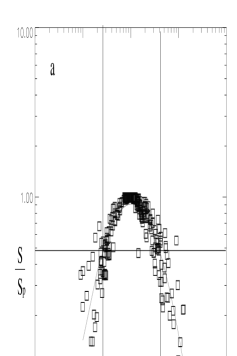
Figure 2: Canonical radio spectra computed for radio sources with $V$$<$3 (top panel); radio sources with $V$$>$3 (bottom panel). The continuous line indicates the least-square fit to the data.

On the other hand, among the 14 sources with $V$$>$3 (Section 3.2) we find 3 objects in which the turnover frequency shows a remarkable change, although the overall radio spectrum maintains a convex shape. Two of these sources (the quasars J1645+6330 and J2024+1718) show a large drop in the peak frequency. We estimate the size of the emitting region by two independent methods. In one case, we use the relationship from O’Dea (odea98 (1998)):

${\rm log}\nu_{\rm p}=-0.21-0.65{\rm log}LS$

which relates the intrinsic spectral peak and the linear size. In the other one, we assume synchrotron self-absorption theory (Kellerman & Pauliny-Toth kpt81 (1981)), in which:

$$\theta=B^{\frac{1}{4}}S_{p}^{\frac{1}{2}}\nu_{p}^{-\frac{5}{4}}(1+z)^{\frac{1}{4}}$$ (2)

where $B$ is the magnetic field, $S_{p}$ the peak flux density, $\nu_{p}$ the turnover frequency and $z$ the redshift. For the magnetic field we consider the values reported by Orienti et al. (mo06 (2006)), obtained assuming equipartition conditions.
As will be discussed in more detail in the following section, if we assume that the magnetic field is frozen within an adiabatically-expanding homogeneous region, its value can be considered constant during the 5 years that elapsed between the most distantly separate observing runs.
The increment in size obtained in both ways are in good agreement, and corresponds to an expansion velocity $\geq$ $c$, which is clearly unrealistic for unboosted young objects. We conclude that such sources are beamed objects and we reject them as genuine candidate HFPs.
The other object, the BL Lac J1751+0939, shows an increment of the peak frequency (from 8.5 to 29 GHz), which can be interpreted in terms of different knots in the jet base dominating the radio emission at the two epochs. This source has a well known history of flux density and spectral variability, and therefore there is no doubt about its blazar nature.
In general, the observed peak frequency of galaxies and quasars are similar as a consequence of the selection criteria. However, if we consider the intrinsic turnover frequency, the KS test finds a clear difference ($>$99%) concerning:
a) galaxies and quasars;
b) the parsec-scale structure depending on its having the CSO-like morphology typical of young radio sources (Orienti et al. mo06 (2006)).
While in the former case the different distribution is easily explained in terms of redshift (quasars are found at higher redshifts than galaxies), in the latter, such a segregation is likely to be indicating two different source populations.
In order to analyze the spectral shape of our sample sources, we construct a canonical radio spectrum for sources with either $V$$<$3 (Fig. 2a) or $V$$>$3 (Fig. 2b).
Following the work of de Vries et al. (dv97 (1997)), the canonical radio spectra have been obtained by normalizing the observed frequencies and fluxes by the source peak frequency and the peak flux density, computed averaging all the epochs:

$$\nu=\frac{1}{m}\sum_{i=1}^{m}\frac{\nu_{i}}{\nu_{p\,i}}$$ (3)

$$S=\frac{1}{m}\sum_{i=1}^{m}\frac{S_{i}}{S_{p\,i}}$$ (4)

where $\nu$ and $S$ are the average normalized frequency and flux density respectively. $\nu_{i}$ and $\nu_{p\,i}$ are the observed frequency and the observed turnover frequency at the i-th epoch, while $S_{i}$ and $S_{p\,i}$ are the observed flux density and the observed peak flux density at the i-th epoch, and $m$ the epochs available.
Sources with $V$$<$3 or $V$$>$3 display different canonical spectral shape. The former have a quite convex spectrum, with a narrow width (FWHM $\sim$1.7). The spectral indices are: $\alpha_{\rm thick}$ $\sim$-0.9$\pm$0.1 and $\alpha_{\rm thin}$ $\sim$ 0.7$\pm$0.1.
The latter have a flatter spectral shape, with a FWHM $\sim$3.6 and spectral indices: $\alpha_{\rm thick}$ $\sim$-0.4$\pm$0.1 and $\alpha_{\rm thin}$ $\sim$ 0.4$\pm$0.1.

Source	Morph.	$\nu_{\rm ep1}$	$\nu_{\rm ep2}$	$\nu_{\rm ep3}$	$\nu_{\rm ep4}$	Vep1	Vep2	Var.
(1)	(2)	(3)	(4)	(5)	(6)	(7)	(8)	(9)
J0003+2129	CSO	5.7$\pm$0.1	5.4$\pm$0.1	5.2$\pm$0.9	5.29$\pm$0.02	2.67d	3.32e	H
J0005+0524	CSO	4.13$\pm$0.09	3.40$\pm$0.09	3.6$\pm$0.7	3.5$\pm$0.7	1.65c	2.1e6	H
J0037+1109	CSO	5.9$\pm$0.1	6.2$\pm$0.2	6.2$\pm$0.7	6.0$\pm$0.7	1.03c	1.47e	H
J0111+3906	CSO	4.76$\pm$0.06	4.68$\pm$0.07	4.66$\pm$0.19		4.63c		H
J0116+2422	Un	5.1$\pm$0.1	6.3$\pm$0.3	6.0$\pm$0.8	6.0$\pm$1.1	4.93c	3.73e	V
J0217+0144	Un	18$\pm$1	flat	flat	flat	94.72c	94.10e	F
J0329+3510	CJ	6.7$\pm$0.3	flat	flat	flat	4.31d	24.43g	F
J0357+2319	Un	12$\pm$1	flat	flat	flat	12.67d	42.48g	F
J0428+3259	CSO	7.3$\pm$0.2	6.8$\pm$0.2	6.9$\pm$0.5	6.55$\pm$0.38	1.12d	2.40g	H
J0519+0848	Un	$>$22	7.4$\pm$0.6	7.26$\pm$0.01	flat	13.28c	19.84g	F
J0625+4440	Un	13$\pm$2	7.4$\pm$1.0	flat	flat	18.18c	62.38g	F
J0638+5933	CSO	12$\pm$2	9.2$\pm$0.7	11.35$\pm$0.30	10.22$\pm$0.20	1.79c	3.74g	H
J0642+6758	Un	4.5$\pm$0.1	4.08$\pm$0.08	4.41$\pm$0.46	4.41$\pm$0.54	0.71c	9.18g	V
J0646+4451	MR	15$\pm$2	11.2$\pm$0.6	10.36$\pm$0.09	10.65$\pm$0.05	19.19c	32.44g	V
J0650+6001	CSO	7.6$\pm$0.3	5.2$\pm$0.2	5.23$\pm$0.18	5.45$\pm$0.15	2.89c	3.12g	V
J0655+4100	Un	7.8		flat	flat	0.46c	3.73g	F
J0722+3722	MR	4.3		4.0$\pm$0.7	3.4$\pm$0.6	2.67d	4.76g	H
J0927+3902	CJ	6.9		8.3$\pm$0.1		15.45d		V
J1016+0513	Un	7.1		flat		72.80d		F
J1045+0624	Un	3.7		4.7$\pm$0.5		5.75d		H
J1148+5254	CSO	8.7		7.9$\pm$0.7		9.74a		V
J1335+4542	CSO	5.1$\pm$0.1	4.9$\pm$0.1	5.1$\pm$0.4		4.64a		H
J1335+5844	CSO	6.0$\pm$0.2	5.5$\pm$0.1	6.50$\pm$0.34		2.84a		H
J1407+2827	CSO	5.34$\pm$0.05	5.01$\pm$0.08	4.95$\pm$0.01		2.02b		H
J1412+1334	Un	4.7$\pm$0.1	4.18$\pm$0.09	4.3$\pm$0.5		0.97b		H
J1424+2256	Un	4.13$\pm$0.07	3.94$\pm$0.06	3.7$\pm$0.3		8.80b		V
J1430+1043	MR	6.5$\pm$0.2	5.7$\pm$0.1	6.2$\pm$0.1		1.37b		H
J1505+0326	Un	7.1$\pm$0.4	6.8$\pm$0.4	flat		30.13b		F
J1511+0518	CSO	11.1$\pm$0.4	10.8$\pm$0.4	10.10$\pm$0.04		10.24b		V
J1526+6650	MR	5.7$\pm$0.1	5.5$\pm$0.1	5.5$\pm$0.9		2.04d		H
J1623+6624	Un	6.0$\pm$0.2	6.0$\pm$0.2	5.1$\pm$0.8	4.5$\pm$0.5	0.87d	11.16i	V
J1645+6330	Un	14$\pm$2	10.1$\pm$0.7	6.0$\pm$0.1	6.8$\pm$0.3	12.38d	21.61i	V
J1717+1917	Un	11.5		flat		81.23h		F
J1735+5049	CSO	6.4$\pm$0.2	6.3$\pm$0.3	5.6$\pm$0.2	5.6$\pm$0.2	0.27h	2.07i	H
J1751+0939	CJ	8.5		29.02$\pm$0.04		8.75h		V
J1800+3848	Un	17$\pm$3	13$\pm$1	13.1$\pm$0.1		1.92f		H
J1840+3900	Un	5.7$\pm$0.5	5.2$\pm$0.4	flat		6.87f		F
J1850+2825	MR	9.1$\pm$0.3	9.5$\pm$0.3	9.9$\pm$0.4		2.15f		V
J1855+3742	CSO	4.00$\pm$0.07	3.81$\pm$0.06	4.0$\pm$0.5		1.32f		H
J2021+0515	CJ	3.75$\pm$0.08	4.5$\pm$0.1	3.7$\pm$0.3		9.94f		V
J2024+1718	Un	14$\pm$2	8.6$\pm$0.4	6.6$\pm$0.4		14.51f		V
J2101+0341	Un	17$\pm$2	3.7$\pm$0.2	flat	flat	28.29c	17.00f	F
J2114+2832	CJ	9.8		flat		34.76d		V
J2123+0535	CJ	18$\pm$4	flat	flat		112.74f		F

Table 3: Peak frequencies and flux density variability between the different epochs of the 51 sources observed with the VLA during the observing runs presented in this paper. The variability indices have been computed by comparing the flux densities measured at each epoch with the mean value obtained by averaging all the available observing epochs, as described in Section 3.2 (see Col. 7 and 8). Col. 1: source name (J2000); Col. 2: Morphological classification from pc-scale information (Orienti et al. mo06 (2006)) Col. 3 and 4: peak frequency of the first two epochs (Dallacasa et al. dd00 (2000); Tinti et al. st05 (2005)); Col. 5 and 6: peak frequency from these new VLA data. Col. 7 and 8: the variability index computed by comparing the flux densities measured in 2003/2004 and presented in this paper with those averaged on all the available epochs, as described in Section 3.2. Since the data flux densities used in Column 7 and 8 were collected during different observing runs, near the value of the variability we report also the observation code from Table 1, which indicates for each source the date of the observations. Col. 9: The classification of the source spectra: H= sources without significant variability, see Section 3.2; V= variable (i.e. with a variability index V$>$3, as defined in Section 3.2 at least during one epoch); F= flat spectrum (i.e. sources with a flat spectrum at least during one epoch; see Section 3.1). Sources marked in boldface are those still considered candidate HFPs.

Source	Morph.	$\nu_{\rm ep1}$	$\nu_{\rm ep2}$	$\nu_{\rm ep3}$	$\nu_{\rm ep4}$	Vep1	Vep2	Var.
(1)	(2)	(3)	(4)	(5)	(6)	(7)	(8)	(9)
J2136+0041	CJ	5.0		5.52$\pm$0.01	5.73$\pm$0.02	2.88c	0.37f	H
J2203+1007	CSO	4.86$\pm$0.07	5.0$\pm$0.1	4.6$\pm$0.7		1.94c		H
J2207+1652	Un	7.4$\pm$0.3	3.5$\pm$0.3	flat	flat	36.01d	35.45e	F
J2212+2355	Un	13$\pm$2	9$\pm$1	flat	flat	43.10d	40.29e	F
J2257+0243	Un	$>$22	$>$22	flat	13.6$\pm$0.3	3.27c	1.92e	F
J2320+0513	Un	5.4$\pm$0.2	flat	9.2$\pm$0.2	flat	23.84c	5.75e	F
J2330+3348	MR	5.6$\pm$0.3	flat	flat		18.84d		F

Table 3: Continued.

4 Discussion

A multi-epoch monitoring of the spectral characteristics provides information on the evolution of the radio spectra. From the analysis of the spectral shape we find 12 sources (see Section 3.1) showing a flat spectrum during at least one of the observing epochs presented in this paper, in addition to the 7 flat-spectrum objects already rejected by Tinti et al. (st05 (2005)). By comparing the frequency break obtained at different epochs we also find that in 3 sources (see Section 3.3) the break has noticeably shifted. Such a change can be explained only assuming a beamed nature for these sources, and therefore we reject them from the sample of genuine young HFPs. If we also consider the 7 sources (5 of them even with a flat spectrum) found with a Core-Jet morphology by Orienti et al. (mo06 (2006)) and then rejected, we obtain that only 31 of the 55 sources of the sample can still be considered HFP candidates, and they are marked in boldface in Table 3.

Although the identification of contaminant objects is the main goal, a multi-epoch monitoring program can provide important information on the spectral evolution in young radio sources.
We assume that young radio sources are described by a continuous injection model, where the radio emission is continuously replenished by a constant flow of fresh relativistic particles with a power-law energy distribution. However, the overall spectra of such sources, characterized by a convex shape, show significant departure from the expected classical power-law (S $\propto$ $\nu^{-\alpha}$). The deviations are well explained by two different phenomena: synchrotron self-absorption causes the rising spectrum (S $\propto$ $\nu^{5/2}$) at frequencies below the peak, while synchrotron losses steepen the spectrum (S $\propto$ $\nu^{-(\alpha+0.5)}$) at high frequencies (Pacholczyk pacho70 (1970)). In very young radio sources such as the HFPs, such a steepening of the spectrum occurs at very high frequency implying that synchrotron losses cannot be investigated with our VLA observations.
In the following discussion we investigate the nature of the radio spectrum and its evolution.

4.1 Adiabatic expansion

At frequencies below the turnover, the adiabatic expansion is the main mechanism that influences the spectral evolution.
In this regime we have:

$$S(\nu)\propto B^{-\frac{1}{2}}\nu^{\frac{5}{2}}\theta^{2}$$ (5)

where $B$ is the magnetic field, $\nu$ the frequency and $\theta$ the angular size of the emitting region.
As the radio source adiabatically expands, the opacity decreases, the turnover moves to lower frequency and the flux density increases.
Is it possible to detect such an increment in our multi-epoch spectra?
First, we assume that the radio emission is due to a homogeneous component that is adiabatically expanding at a constant rate:

$$\theta=\theta_{0}\left(\frac{t_{0}+\Delta t}{t_{0}}\right)$$ (6)

where $\theta_{0}$ is the angular size at the time $t_{0}$, and $\theta$ at the time $t_{0}$+$\Delta t$, and the magnetic field is frozen in the plasma:

$$B=B_{0}\left(\frac{t_{0}}{t_{0}+\Delta t}\right)^{2}$$ (7)

where $B_{0}$ is the magnetic field at the epoch $t_{0}$, while $B$ is at the time $t_{0}+\Delta t$.
From Equation 5, the flux density at the frequency $\nu$ at a given time $t$ is:

$$S\propto B_{0}^{-\frac{1}{2}}\nu^{\frac{5}{2}}\theta_{0}^{2}\left(\frac{t_{0}+\Delta t}{t_{0}}\right)^{3}.$$ (8)

The turnover frequency is:

$$\nu_{\rm t,0}\propto B_{0}E_{0}^{2}$$ (9)

where $E_{0}$ is the energy of the relativistic particles. During the expansion of the homogeneous synchrotron-emitting region $E\propto t^{-1}$ (Pacholczyk pacho70 (1970)), which implies that

$$\nu_{\rm t,1}=\nu_{\rm t,0}\left(\frac{t_{0}}{t_{0}+\Delta t}\right)^{4}.$$ (10)

If $t-t_{0}$=$\Delta t$ $\ll$ $t_{0}$, the flux density and the turnover frequency can be considered approximately constant. We consider $\Delta t$ $\sim$ 5 years (the time elapsed between the first and last observing run), and $t_{0}$ $>$ 15 years, since all the sources are part of the 87GB sample. If $t_{0}$ = 20 years, we expect a flux density increment of a factor of $\sim$ 2 in the optically thick part of the spectra. Such an increment becomes undetectable for sources with ages of $\sim$ 100 years. On the other hand, the $\nu_{t}$ should have decreased by about 70% of its previous value. If $t_{0}$ $\sim$ 100 years, the decrement should be less than 20% of its previous value, i.e. a turnover frequency of 22 GHz moves to 18 GHz, making the detection rather difficult due to the poor frequency coverage available. This result is based on the strong assumptions that the magnetic field is frozen in a homogeneous component which is adiabatically expanding. However, it is possible that either the time-variable magnetic field is not frozen in the plasma, or the radio emitting region is not homogeneous. In both cases the flux density increment and the frequency decrement are expected to be even less significant.
Therefore, we conclude that adiabatic expansion is not able to produce any significant changes in the optically thick part of the spectrum detectable in our multi-epoch observations, perhaps with the exception of a few sources, such as J0650+6001 (Section 4.3) where a tentative flux density increment at a frequency below the spectral peak has been found, or the “faint” HFP J1459+3337 (Orienti & Dallacasa, submitted).

4.2 The nature of the overall spectra

In the previous Sections we have assumed that the radio emission is due to a partially opaque electron synchrotron radiation which originates within a homogeneous region. Variations in the opacity throughout the emitting region lead to an overall spectrum which is the superposition of the spectra of many single regions.
Figure 3 shows the overall spectrum (diamonds) of J0650+6001 and J1511+0518, together with the spectra of each single component (squares and crosses), as revealed by VLBI observations (Orienti et al. mo06 (2006)). In both sources, pc-scale resolution images show that the radio emission originates within two main components, which can be interpreted as the lobes of a mini radio source.
The overall spectra are easily explained as the result of the superposition of the spectra of individual components. In both sources, the two radio emitting regions have different turnover frequencies, and, thus, different parts of the overall spectra are influenced more by one component, rather than the other, as is easily seen in the case of J1511+0518. As a consequence, changes in the total spectra may strongly depend on the evolution of the emission of each single component.
The variation of the total spectrum that occurred over 5 years makes J0650+6001 an interesting case study.
If we compare the overall spectra measured at different epochs, we find that at 1.4 GHz, well below the peak frequency, the flux density appears to be increasing, although within the errors, as expected by adiabatic expansion.
On the other hand, at frequencies higher than the peak the flux density decreases. During the first epoch of observation, the optically thin spectrum was described by a power-law with $\alpha$ $\sim$ 0.3, while during the subsequent observing runs it displayed $\alpha$ $\sim$ 0.7. Such a steepening cannot be directly related to a shift of the break frequency of the overall spectrum, but is rather due to the evolution of the spectra of the individual components.

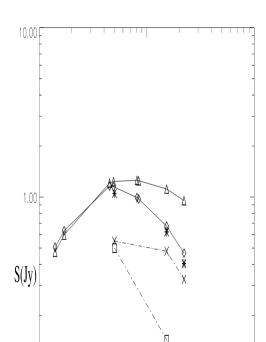
Figure 3: The spectra of the sources J0650+6001 (top) and J1511+0518 (bottom): diamonds represent the overall spectrum obtained with these new VLA observations, while crosses and squares represent the spectra of the two source components (Xiang et al. xiang02 (2002); Xu et al. xu95 (1995); Orienti et al. mo06 (2006)). In the case of J0650+6001, triangles show the overall spectrum from Dallacasa et al. (dd00 (2000)). The asterisks represent the sum of the spectra of the single components. In the case of J1511+0518 not all the flux density could be recovered by VLBI images (Orienti et al. mo06 (2006)).

5 Conclusions

We have presented the results of new epochs of high-sensitivity simultaneous multi-frequency VLA observations of a sample of young HFP candidates. By considering the spectral shape and the change of the frequency break we find 15 sources which turned out to be blazar objects, in addition to the 7 already found with a flat spectrum by Tinti et al. (st05 (2005)). If we consider also the 7 sources rejected by Orienti et al. (mo06 (2006)) on the basis of their Core-Jet morphology, and 5 of them also with a flat spectrum, we find that 24 of the 55 sources from the HFP sample are contaminant blazar objects, and thus only 31 objects ($\sim$56%) can still be considered HFP candidates.
The comparison of the variability properties with the optical identification have shown that quasars and galaxies display different characteristics. If in the case of the turnover frequency distribution such a segregation is due to redshift ranges (quasars are found at systematically higher redshifts than galaxies), the difference in the variability index likely reflects two kinds of radio source populations. An even stronger segregation in the flux-density and spectral-shape variability is found between objects with or without a CSO-like morphology.
Since polarization properties are another effective tool to discriminate young radio sources from contaminant blazars, polarimetric data concerning the sources of the “bright” HFP sample have been studied, and they will be presented in a companion paper (Orienti & Dallacasa 2007, Paper II).
Making use of the several epochs available, we have tried to investigate the spectral evolution of the radio emission of genuine young radio sources.
At frequencies below the peak the spectral evolution is dominated by adiabatic expansion, and we would expect a flux density increment, while at frequencies above the spectral peak, in addition to the decrease of the flux density due to adiabatic expansion, synchrotron losses also may play a role. Considering the time elapsed between the two farthest spaced observing runs (5 years), we conclude that a variation in the optically-thick part of the overall spectrum would have been detected only if the radio emission would have started very recently, i.e. $\sim$ 20 years, which is statistically unlikely for the sources in the sample.
On the other hand, as seen in the analysis of the spectra of individual objects, there are a few cases, such as the source J0650+6001, with spectral variations. However, if we consider that the radio emission comes from a single homogeneous region, we are not able to explain such changes. Combining the low-resolution, flux density information provided by VLA observations with the pc-scale resolution from VLBA data, we can describe the total radio spectrum as the result of the superposition of the spectra of different emitting regions.
In general, to determine the evolution of the radio emission, we must resolve each single source component.
For this, new simultaneous multi-frequency VLBA observations in both the optically thick and thin parts of the spectrum have been carried out for 5 genuine HFPs, with a CSO-like morphology. The analysis of the radio spectrum of each single component will enable us to set strong constraints on the fate of the radio emission.

- (1) Alexander, P. 2000, MNRAS, 319, 8
- (2) Bicknell, G.V., Dopita, M.A., O’Dea, C.P.O. 1997, ApJ, 485, 112
- (3) Browne, I.W.A., Patnaik, A.R., Wilkinson, P.N., Wrobel, J.A. 1998, MNRAS, 293, 257
- (4) Dallacasa, D., Stanghellini, C., Centonza, M., Fanti, R. 2000, A&A, 363, 887
- (5) Dallacasa, D. 2003, PASA, 20, 79
- (6) de Vries, W.H., Barthel, P.D., O’Dea, C.P. 1997, A&A, 321, 105
- (7) Fanti, C., Fanti, R., Dallacasa, D., Schilizzi, R.T. et al. 1995, A&A, 302, 317
- (8) Kameno, S., Horiuchi, S., Shen, Z.-Q. et al. 2000, PASJ, 52, 209
- (9) Kellerman, K.I., Pauliny-Toth, I.I.K. 1981, ARA&A, 19, 373
- (10) Marecki, A., Spencer, R.E., Kunert, M. 2003, PASA, 20. 46
- (11) Murgia, M. 2003, PASA, 20, 19
- (12) O’Dea, C.P., Baum, S.A. 1997, AJ, 113, 148
- (13) O’Dea, C.P. 1998, PASP, 110, 493
- (14) Orienti, M., Dallacasa, D., Tinti, S., Stanghellini. C. 2006, A&A, 450, 959
- (15) Orienti, M., Dallacasa, D., Stanghellini, C. 2007, A&A, 461, 923
- (16) Orienti , M., Dallacasa, D. 2007, A&A, submitted
- (17) Pacholczyk, A.G. 1970, Radio Astrophysics, (San Francisco: Freeman & Co.)
- (18) Patnaik, A.R., Browne, I.W.A., Wilkinson, P.N., Wrobel, J.M. 1992, MNRAS, 254, 655
- (19) Polatidis, A.G., & Conway, J.E. 2003, PASA, 20, 69
- (20) Readhead, A.C.S., Taylor, G.B., Xu, W., Pearson, T.J. et al. 1996, ApJ, 460, 612
- (21) Snellen, I.A.G., Schilizzi, R.T., Miley, G.K. et al. 2000, MNRAS, 319, 445
- (22) Stanghellini, C., O’Dea, C.P., Dallacasa, D. et al. 2005, A&A, 443, 891
- (23) Tinti, S., Dallacasa, D., de Zotti, G., Celotti, A., Stanghellini, C. 2005, A&A, 432,31
- (24) Torniainen, I., Tornikoski, M., Teräsranta, H., Aller, H.D. 2005, A&A, 435, 839
- (25) Torniainen, I., Tornikoski, M., Lähteenmäki, A., et al. 2007, A&A, 469, 451
- (26) Wilkinson, P.N., Polatidis, A.G., Readhead, A.C.S., Xu, W., Pearson, T.J. 1994, ApJ, 432, 87
- (27) Wilkinson, P.N., Browne, I.W.A., Patnaik, A.R. et al. 1998, MNRAS, 300, 790
- (28) Xiang, L., Stanghellini, C., Dallacasa, D., Haiyan, Z. 2002, A&A, 385, 768
- (29) Xu,W., Readhead, A.C.S., Pearson, T.J., Polatidis, A.G., Wilkinson, P.N. 1995, ApJS, 99, 279