Circular dielectric cavity and its deformations

Abstract

The construction of perturbation series for slightly deformed dielectric circular cavity is discussed in details. The obtained formulae are checked on the example of cut disks. A good agreement is found with direct numerical simulations and far-field experiments.

I Introduction

Dielectric micro-cavities are now widely used as micro-resonators and micro-lasers in different physical, chemical and biological applications (see e.g. vahala , krioukov and references therein). The principal object of these studies is the optical emission from thin dielectric micro-cavities of different shapes stonescience . Schematically such cavity can be represented as a cylinder whose height is small in comparison with its transverse dimensions (see Fig. 1).

Figure 1: Schematic representation of a dielectric cavity.

If the refractive index of the cavity is $n_{1}$ and the cavity is surrounded by a material with the refractive index $n_{2}<n_{1}$ (we assume that the permeabilities in both media are the same) the time-independent Maxwell’s equations take the form (see e.g. jackson )

$$\vec{\nabla}\cdot\vec{B}_{j}=0\ , \vec{\nabla}\cdot n_{j}^{2}\vec{E}_{j}=0\ ,$$

$$\vec{\nabla}\times\vec{B}_{j}=-in_{j}^{2}k\vec{E}_{j}\ , \vec{\nabla}\times\vec{E}_{j}=ik\vec{B}_{j}$$ (1)

where the subscript $j=1$ (resp. $j=2$) denotes points inside (resp. outside) the cavity and $k$ is the wave vector in the vacuum. These equations have to be completed by the boundary conditions which follow from the continuity of normal $\vec{B}_{\nu}$ and $n\vec{E}_{\nu}$ and tangential $\vec{E}_{\tau}$ and $\vec{B}_{\tau}$ components

$$n_{1}^{2}\vec{E}_{1\nu}=n_{2}^{2}\vec{E}_{2\nu}\ ,\ \vec{B}_{1\nu}=\vec{B}_{2\nu}\ ,\ \vec{E}_{1\tau}=\vec{E}_{2\tau}\ ,\ \vec{B}_{1\tau}=\vec{B}_{2\tau}\ .$$

In the true cylindrical geometry, the $z$-dependence of electromagnetic fields is pure exponential: $\sim{\rm e}^{{\rm i}qz}$. Then the above Maxwell equations can be reduced to the 2-dimensional Helmholtz equations for the electric field, $E_{jz}$, and the magnetic field $B_{jz}$ along the axe of the cylinder

$$(\Delta+\tilde{n}_{j}^{2}k^{2})~{}E_{jz}(x,y)=0\ ,\ (\Delta+\tilde{n}_{j}^{2}k^{2})~{}B_{jz}(x,y)=0$$ (2)

with the following boundary conditions

$$E_{1z}=E_{2z},B_{1z}=B_{2z},\frac{\partial E_{1z}}{\partial\tau}=\frac{\partial E_{2z}}{\partial\tau},\frac{\partial B_{1z}}{\partial\tau}=\frac{\partial B_{2z}}{\partial\tau},$$

and

$$\frac{1}{\tilde{n}_{1}^{2}}\frac{\partial B_{1z}}{\partial\nu}-\frac{1}{\tilde{n}_{2}^{2}}\frac{\partial B_{2z}}{\partial\nu} = \frac{q(n_{2}^{2}-n_{1}^{2})}{k\tilde{n}_{1}^{2}\tilde{n}_{2}^{2}}\frac{\partial E_{z}}{\partial\tau}\ ,$$

$$\frac{n_{1}^{2}}{\tilde{n}_{1}^{2}}\frac{\partial E_{1z}}{\partial\nu}-\frac{n_{2}^{2}}{\tilde{n}_{2}^{2}}\frac{\partial E_{2z}}{\partial\nu} = \frac{q(n_{2}^{2}-n_{1}^{2})}{k\tilde{n}_{1}^{2}\tilde{n}_{2}^{2}}\frac{\partial B_{z}}{\partial\tau}\ .$$ (3)

Here $\tilde{n}_{j}^{2}=n_{j}^{2}-q^{2}/k^{2}$ plays the role of the effective two-dimensional (in the $x-y$ plane) refractive index.

When fields are independent on $z$ (i.e. $q=0$) boundary conditions (3) do not mix $B_{z}$ and $E_{z}$ and the two polarizations are decoupled. They are called transverse electric (TE) field when $E_{z}=0$ and transverse magnetic (TM) field when $B_{z}=0$. Both cases are described by the scalar equations

$$(\Delta+\tilde{n}_{j}^{2}k^{2})~{}\Psi_{j}(x,y)=0$$ (4)

where $\Psi(x,y)$ stands for electric (TM) or magnetic (TE) fields with the following conditions on the interface between both media: $\Psi_{1}=\Psi_{2}$ and

$$\frac{\partial\Psi_{1}}{\partial\nu}=\frac{\partial\Psi_{2}}{\partial\nu} \mbox{ for TM polarization}\ ,$$ (5)

$$\frac{1}{n_{1}^{2}}\frac{\partial\Psi_{1}}{\partial\nu}=\frac{1}{n_{2}^{2}}\frac{\partial\Psi_{2}}{\partial\nu} \mbox{ for TE polarization}\ .$$ (6)

These equations are, strictly speaking, valid only for an infinite cylinder but they are widely used for a thin dielectric cavities by introducing the effective refractive index corresponding to the propagation of confined modes in the bulk of the cavity (see e.g. cavity ). In practice, it reduces to small changes in the refractive indices (which nevertheless is of importance for careful comparison with experiment polygons ). For simplicity we will consider below two-dimensional equations (4) as the exact ones.

Only in very limited cases, these equations can be solved analytically. The most known case is the circular cavity (the disk) where variables are separated in polar coordinates. For other cavity shapes tedious numerical simulations are necessary.

The purpose of this paper is to develop perturbation series for quasi-stationary spectrum and corresponding wave functions for general cavities which are small deformations of the disk. The obtained formulae are valid when an expansion parameter is small enough. The simplicity, the generality, and the physical transparency of the results make such approach of importance for technological and experimental applications.

The plan of the paper is the following. In Section II the calculation of quasi-stationary states for a circular cavity is reviewed for completeness. Special attention is given to certain properties rarely mentioned in the literature. The construction of perturbation series for eigenvalues and eigenfunctions of small perturbations of circular cavity boundary is discussed in Section III. The conditions of applicability of perturbation expansions are discussed in Section IV. The obtained general formulae are then applied to the case of cut disks in Section V. Some technical details are collected in Appendices.

II Dielectric disk

Let us consider a two dimensional circular cavity of radius $R$ made of a material with $n>1$ refractive index. The region outside the cavity is assumed to be the air with a refractive index of one. The two-dimensional equations (4) for this cavity are

$$(\Delta+n^{2}k^{2})\Psi = 0\;\mbox{ when }r\leq R\ ,$$

$$(\Delta+k^{2})\Psi = 0\;\mbox{ when }r>R\ .$$ (7)

There is no true bound states for dielectric cavities. The physical origin of the existence of long lived quasi-bound states is the total internal reflection of rays with the incidence angle bigger than the critical angle

$$\theta_{c}=\arcsin\frac{1}{n}\ .$$ (8)

To investigate quasi-bound states one imposes outgoing boundary condition at infinity, namely, we require that far from the cavity there exist only outgoing waves

$$\Psi(\vec{x}\ )\propto{\rm e}^{{\rm i}k|\vec{x}\,|}\;\mbox{ when }|\vec{x}\,|\to\infty\ .$$

In cylindrical coordinates $(r,\theta)$, the general form of the solutions is the following

$$\Psi(r,\theta)=\left\{\begin{array}[]{ll}a_{m}J_{m}(nkr){\rm e}^{{\rm i}m\theta}\ ,&r\leq R\ ,\\ b_{m}H_{m}^{(1)}(kr){\rm e}^{{\rm i}m\theta}\ ,&r>R\ ,\end{array}\right.$$ (9)

where $m=0,1,\ldots$ is an integer (the azimuthal quantum number) related to the orbital momentum. $J_{m}(x)$ (resp.$H_{m}^{(1)}(x)$) stands for the Bessel function (resp. the Hankel function of the first kind) of order $m$. Due to rotational symmetry, eigenvalues with $m\neq 0$ are doubly degenerated.

By imposing the boundary conditions (5) or (6) one gets the quantization condition

$$\frac{n}{\nu}\frac{J_{m}^{\prime}}{J_{m}}(nkR)=\frac{H_{m}^{(1)\prime}}{H_{m}^{(1)}}(kR)$$ (10)

where

$$\nu=\left\{\begin{array}[]{cc}1&\mbox{ for TM polarization}\\ n^{2}&\mbox{ for TE polarization}\end{array}\right.\ .$$ (11)

The quasi-stationary eigenvalues of this problem depend on azimuthal quantum number $m$ and on other quantum number $p$ related with radial momentum: $k=k_{mp}$. They are complex numbers

$$k=k_{r}+{\rm i}k_{i}$$ (12)

where $k_{r}$ determines the position of a resonance and $k_{i}<0$ is related with its lifetime.

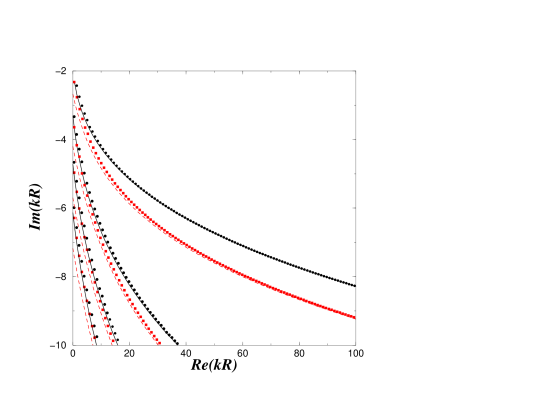
In Fig. 2 we plot solutions of Eq. (10) obtained numerically for a cylindrical cavity with refractive index $n=1.5$. Points are organized in families corresponding to different values of radial quantum number $p$.

a)

b)

Figure 2: Quasi-stationary eigenvalues for a circular cavity with $n=1.5$. a) TM polarization, b) TE polarization. Filled circles are deduced from direct numerical resolution of Eq. (10), while open squares indicate semiclassical approximation for these eigenvalues based on Eqs. (16) and (17) when $|kR|<m<n|kR|$.

The dotted line in these figures indicates the classical lifetime of modes with fixed $m$ and $k\to\infty$. Physically these modes correspond to waves propagating along the diameter whose lifetime is given by

$${\rm Im}(kR)=\frac{1}{2n}\ln\left(\frac{n-1}{n+1}\right)\simeq-0.53648$$ (13)

In the semiclassical limit and for Im$(kR)\ll$ Re$(kR)$ simple approximate formulae can be obtained from standard approximation of Bessel and Hankel functions bateman :

• when $m<z$

  $$J_{m}(z)=\sqrt{\frac{2}{\pi}}\frac{1}{(z^{2}-m^{2})^{1/4}}$$ (14)

  $$\times \cos\left(\sqrt{z^{2}-m^{2}}-m\arccos{\frac{m}{z}}-\frac{\pi}{4}\right)\ ,$$

• when $m>z$

  $$H_{m}^{(1)}(z)=-{\rm i}\sqrt{\frac{2}{\pi}}\frac{{\rm e}^{-\sqrt{m^{2}-z^{2}}}}{(m^{2}-z^{2})^{1/4}}$$ (15)

  $$\times \left(\frac{m}{z}+\sqrt{\left(\frac{m}{z}\right)^{2}-1}\right)^{m}\ .$$

Denoting $x={\rm Re}(kR)$ and $y={\rm Im}(kR)$ and assuming that $y\ll x$, $x\gg 1$, and $m/n<x<m$ one gets (see e.g. nockel ) that the real part of (10) can be transformed to the following form

$$\sqrt{n^{2}x^{2}-m^{2}}-m\arccos{\frac{m}{nx}}-\frac{\pi}{4}$$

$$=\arctan\nu\sqrt{\frac{m^{2}-x^{2}}{n^{2}x^{2}-m^{2}}}+(p-1)\pi$$ (16)

where the integer $p=1,2,\ldots$ is the radial quantum number and $\nu$ is defined in (11). The imaginary part of equation (10) is then reduced to

$$y\approx-\frac{2}{\pi x(n^{2}-1)|H_{m}^{(1)}(x)|^{2}}\zeta$$ (17)

where $\zeta=1$ for TM waves and $\zeta=n^{2}x^{2}/(m^{2}(n^{2}+1)-n^{2}x^{2})$ for TE waves. When $x$ and $m$ are large, $y$ is exponentially small as it follows from (15).

The above equations can not be applied for the most confined levels (similar to the “whispering gallery” modes in closed billiards) for which $nx$ is close to $m$. In Appendix A it is shown that real part of such quasi-stationary eigenvalues with ${\cal O}(m^{-1})$ precision is given by the following expression

$$x_{m,p}=\frac{m}{n}+\frac{\eta_{p}}{n}\Big{(}\frac{m}{2}\Big{)}^{1/3}-\frac{1}{\nu\sqrt{n^{2}-1}}$$ (18)

$$+\frac{3\eta_{p}^{2}}{20n}\Big{(}\frac{2}{m}\Big{)}^{1/3}+\frac{n^{2}\eta_{p}}{2\nu(n^{2}-1)^{3/2}}\Big{(}\frac{2}{3\nu^{2}}-1\Big{)}\Big{(}\frac{2}{m}\Big{)}^{2/3}$$

where $\eta_{p}$ is the modulus of the $p^{\mbox{th}}$ zero of the Airy function (90).

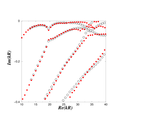
A more careful study of (10) reveals that there exist other branches of eigenvalues with large imaginary part not visible in Fig. 2. Some of them are indicated in Fig. 3.

Figure 3: Additional branches of quasi-stationary eigenvalues for a circular cavity with $n=1.5$. Black circles indicate the TM modes and red squares show the position of the TE modes. Solid black and dashed red lines represent the asymptotic result (19) for respectively the TM and the TE modes.

These states can be called external whispering gallery modes as their wave functions are practically zero inside the circle. So they are of minor importance for our purposes. They can also be identified with above-barrier resonances. In Appendix A it is shown that in semiclassical limit these states are related with complex zeros of the Hankel functions and they are well described asymptotically (with ${\cal O}(m^{-1})$ error) as follows

$$x_{m,p}=m+\left(\frac{m}{2}\right)^{1/3}\eta_{p}\ {\rm e}^{-2{\rm i}\pi/3}-\frac{{\rm i}\nu}{\sqrt{n^{2}-1}}$$

$$+\frac{3{\rm e}^{-4{\rm i}\pi/3}\eta_{p}^{2}}{20}\left(\frac{2}{m}\right)^{1/3}$$

$$+\frac{{\rm i}\nu\eta_{p}{\rm e}^{-2{\rm i}\pi/3}}{2(n^{2}-1)^{3/2}}\left(1-\frac{2}{3}\nu^{2}\right)\left(\frac{2}{m}\right)^{2/3}$$ (19)

with the same $\eta_{p}$ as in (18).

Similar equations have been obtained in henning .

III Perturbation treatment of deformed circular cavities

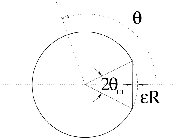
In the previous Section we have considered the case of a dielectric circular cavity. It is one of the rare cases of integrable dielectric cavities in two dimensions. The purpose of this Section is to develop a perturbation treatment for a general cavity shape which is a small deformation of the circle (see Fig.4).

Figure 4: Example of a deformed circular cavity. Shaded areas represent regions where the refractive index differs from the one of the circular cavity.

We consider a cavity which boundary is defined as

$$r=R+\lambda f(\theta)$$ (20)

in the polar coordinates $(r,\theta)$. Here $\lambda$ is a formal small parameter aiming at arranging perturbation series.

Our main assumption is that the deformation function $\lambda f(\theta)$ is small

$$|\lambda f(\theta)|\ll R\ .$$ (21)

Of course, for the quantum mechanical perturbation theory this condition is not enough. It is quite natural (and will be demonstrated below) that the criterion of applicability of the quantum perturbation theory is, roughly,

$$\delta a\ k^{2}\ll 1$$ (22)

where $\delta a$ is the area where perturbation ’potential’ $\delta n^{2}$ is non zero (represented by dashed regions in Fig. 4).

To construct the perturbation series for the quasi-stationary states, we use two complementary methods. In Section III.1 we adapt the method proposed in yeh ; keller for diffraction problems. The main idea of this method is to impose the required boundary conditions (5) or (6) not along the true boundary of the cavity but on the circle $r=R$. Under the assumption (22) this task can be achieved by perturbation series in $\lambda$. In Section III.2 we use a more standard method based on the direct perturbation solution of the required equations using the Green function of the circular dielectric cavity. Both methods lead to the same series but they stress different points and may be useful in different situations.

For clarity we consider only the TM polarization where the field and its normal derivative are continuous on the dielectric interface. For the TE polarization the calculations are more tedious but follow the same steps. To simplify the discussion we assume that the deformation function $f(\theta)$ is symmetric: $f(-\theta)=f(\theta)$ (as in Fig. 4). In this case the quasi-stationary eigenfunctions are either symmetric or antisymmetric with respect to this inversion. Then in polar coordinates, they can be expanded either in $\cos(p\theta)$ or $\sin(p\theta)$ series. The general case of non-symmetric cavities is analogous to the case of degenerate perturbation series and can be treated correspondingly.

III.1 Boundary shift

The condition of continuity of the wave function at the dielectric interface states

$$\Psi_{1}(R+\lambda f(\theta),\theta)=\Psi_{2}(R+\lambda f(\theta),\theta)$$ (23)

where subscripts $1$ and $2$ refer respectively to wave function inside and outside the cavity. Expanding formally $\Psi_{1,2}$ into powers of $\lambda$ one gets

$$[\Psi_{1}-\Psi_{2}](R,\theta)=-\lambda f(\theta)\left[\frac{\partial\Psi_{1}}{\partial r}-\frac{\partial\Psi_{2}}{\partial r}\right](R,\theta)$$ (24)

$$- \frac{1}{2}\lambda^{2}f^{2}(\theta)\left[\frac{\partial^{2}\Psi_{1}}{\partial r^{2}}-\frac{\partial^{2}\Psi_{2}}{\partial r^{2}}\right](R,\theta)+\ldots\;.$$

For the TM polarization the conditions (5) imply that the derivatives of the wave functions inside and outside the cavity along any direction are the same. Choosing the radial direction, one gets the second boundary condition

$$\frac{\partial\Psi_{1}}{\partial r}(R+\lambda f(\theta),\theta)=\frac{\partial\Psi_{2}}{\partial r}(R+\lambda f(\theta),\theta)$$ (25)

which can be expanded over $\lambda$ as follows

$$\left[\frac{\partial\Psi_{1}}{\partial r}-\frac{\partial\Psi_{2}}{\partial r}\right](R,\theta)=$$

$$- \lambda f(\theta)\left[\frac{\partial^{2}\Psi_{1}}{\partial r^{2}}-\frac{\partial^{2}\Psi_{2}}{\partial r^{2}}\right](R,\theta)$$

$$- \frac{1}{2}\lambda^{2}f^{2}(\theta)\left[\frac{\partial^{3}\Psi_{1}}{\partial r^{3}}-\frac{\partial^{3}\Psi_{2}}{\partial r^{3}}\right](R,\theta)+\ldots\ .$$

We find it convenient to look for the solutions of Eqs. (24) and (III.1) in the following form

$$\Psi_{1}(r,\theta) = \frac{J_{m}(nkr)}{J_{m}(nx)}\cos(m\theta)$$ (27)

$$+ \sum_{p\neq m}a_{p}\frac{J_{p}(nkr)}{J_{p}(nx)}\cos(p\theta)\;,$$

$$\Psi_{2}(r,\theta) = (1+b_{m})\frac{H_{m}^{(1)}(kr)}{H_{m}^{(1)}(x)}\cos(m\theta)$$ (28)

$$+ \sum_{p\neq m}(a_{p}+b_{p})\frac{H_{p}^{(1)}(kr)}{H_{p}^{(1)}(x)}\cos(p\theta)\ .$$

Here and for all which follows, $x$ stands for $kR$. These expressions correspond to symmetric eigenfunctions. For antisymmetric functions all $\cos(\ldots)$ have to be substituted by $\sin(\ldots)$.

From (24) and (III.1) one concludes that the unknown coefficients $a_{p}$, and $b_{p}$ have the following expansions

$$a_{p}=\lambda\alpha_{p}+\lambda^{2}\beta_{p}+\ldots\ ,\;\;b_{p}=\lambda^{2}\gamma_{p}+\ldots\;.$$ (29)

Correspondingly, the quasi-stationary eigenvalue, $kR\equiv x$, can be represented as the following series

$$x=x_{0}+\lambda x_{1}+\lambda^{2}x_{2}+\ldots\;.$$ (30)

Here $x_{0}$ is the complex solution of (10) which we rewrite in the form

$$S_{m}(x_{0})=0$$ (31)

introducing for a further use the notation for all $m$ and $x$

$$S_{m}(x)=n\frac{J_{m}^{\prime}}{J_{m}}(nx)-\frac{H_{m}^{(1)\prime}}{H_{m}^{(1)}}(x)\;.$$ (32)

The explicit construction of these perturbation series is presented in Appendix B. The results are the following. The perturbed eigenvalue (30) is

$$x = x_{0}\Big{[}1-\lambda A_{mm}+\lambda^{2}\Big{(}\frac{1}{2}(3A_{mm}^{2}-B_{mm})$$

$$+ x_{0}(A_{mm}^{2}-B_{mm})\frac{H_{m}^{(1)\prime}}{H_{m}^{(1)}}(x_{0})$$

$$- (n^{2}-1)x_{0}\sum_{k\neq m}A_{mk}\frac{1}{S_{k}(x_{0})}A_{km}\Big{)}\Big{]}+{\cal O}(\lambda^{3})\;.$$

The coefficients of quasi-stationary eigenfunction (27) and (28) are

$$a_{p} = \lambda x_{0}(n^{2}-1)\frac{1}{S_{p}(x_{0})}\Big{[}A_{pm}+\lambda\Big{(}A_{pm}A_{mm}\Big{(}\frac{x_{0}}{S_{p}}\frac{\partial S_{p}}{\partial x}-1\Big{)}$$ (34)

$$+ \frac{1}{2}B_{pm}\Bigg{(}1+x_{0}\Big{(}\frac{H_{m}^{(1)\prime}}{H_{m}^{(1)}}+\frac{H_{p}^{(1)\prime}}{H_{p}^{(1)}}\Big{)}\Bigg{)}+x_{0}(n^{2}-1)\sum_{k\neq m}A_{pk}\frac{1}{S_{k}(x_{0})}A_{km}\Big{)}\Big{]}+{\cal O}(\lambda^{3})$$

and

$$b_{p}=\lambda^{2}\frac{1}{2}x_{0}^{2}(n^{2}-1)B_{pm}+{\cal O}(\lambda^{3})$$ (35)

In these formulae $A_{mn}$ and $B_{mn}$ are the Fourier harmonics of the perturbation function $f(\theta)$ and its square, given by (114) and (119) respectively. The above expressions are quite similar to usual perturbation series and $S_{p}(x_{0})$ plays the role of the energy denominator.

It is instructive to calculate the imaginary part of the perturbed level from the knowledge of the first order terms only. Assuming that Im $(x_{0})\ll$ Re $(x_{0})$ and using the Wronskian relation (see e.g. bateman 7.11.34)

$$H_{m}^{(1)\prime}(x)H_{m}^{(2)}(x)-H_{m}^{(2)\prime}(x)H_{m}^{(1)}(x)=\frac{4{\rm i}}{\pi x}$$ (36)

one gets from (III.1)

$${\rm Im}(x)={\rm Im}(x_{0})(1+\rho)-\lambda^{2}\frac{2x_{0}(n^{2}-1)}{\pi}\sum_{p\neq m}\frac{A_{mp}^{2}}{|S_{p}H_{p}^{(1)}|^{2}}$$ (37)

where (assuming that $m>x_{0}$ so $H_{m}^{(1)\prime}/H_{m}^{(1)}$ is real cf. (15))

$$\rho = -\lambda A_{mm}+\lambda^{2}\left[\frac{1}{2}(3A_{mm}^{2}-B_{mm})\right.$$

$$+ \left.x_{0}(A_{mm}^{2}-B_{mm})\frac{H_{m}^{(1)\prime}}{H_{m}^{(1)}}(x_{0})\right]\ .$$

Expression (37) without the $\rho$ correction (which is multiplied by ${\rm Im}(x_{0})$ and so negligible for well-confined levels) can be independently calculated from the following general considerations. From (7) it follows that inside the cavity

$$n^{2}(k^{2}-k^{*2})\int_{V}|\Psi(x)|^{2}{\rm d}\vec{x}=J$$ (39)

where

$$J=\int_{B}\Big{(}\Psi^{*}\frac{\partial}{\partial\vec{\nu}}\Psi-\Psi\frac{\partial}{\partial\vec{\nu}}\Psi^{*}\Big{)}{\rm d}\vec{\sigma}\ .$$ (40)

In the first integral the integration is performed over the volume of the cavity, $V$, while the second integral is taken over the boundary of the cavity, $B$. $\nu$ is the coordinate normal to the cavity boundary and $J$ represents the current through the boundary. For the TM polarization, it equals the current at infinity.

From (28) and (34) it follows that the field outside the cavity in the first order of the perturbative expansion is

$$\Psi_{2}(r,\theta) = \frac{H_{m}^{(1)}(kr)}{H_{m}^{(1)}(x)}\cos(m\theta)$$

$$+ \lambda(n^{2}-1)x_{0}\sum_{p\neq m}A_{pm}\frac{H_{p}^{(1)}(kr)}{S_{p}(x)H_{p}^{(1)}(x)}\cos(p\theta)\ .$$

The current can be directly calculated from (36) or from the asymptotic of the Hankel functions. Then the current can be written

$$J=4{\rm i}\Big{[}\frac{1}{|H_{m}^{(1)}|^{2}}+\lambda^{2}(n^{2}-1)^{2}x_{0}^{2}\sum_{p\neq m}\frac{A_{pm}^{2}}{|S_{p}H_{m}^{(1)}|^{2}}\Big{]}\ .$$ (42)

To calculate the integral over the cavity volume in the leading order, the non-perturbed function can be used inside the cavity. Then the integration over the circle $r=R$ leads to

$$\int_{V}|\Psi(x)|^{2}{\rm d}\vec{x}\approx\frac{\pi}{J_{m}^{2}(nx_{0})}\int_{0}^{R}J_{m}^{2}(nkr)r{\rm d}r\ .$$ (43)

The last integral is (see bateman 7.14.1)

$$\int_{0}^{R}J_{m}^{2}(nkr)r{\rm d}r$$

$$=\frac{R^{2}}{2}\Big{[}J_{m}^{\prime 2}(nkR)+J_{m}^{2}(nkR)(1-\frac{m^{2}}{(nkR)^{2}})\Big{]}\ .$$

From the eigenvalue equation (10) and the asymptotic (15), it follows that

$$n\frac{J_{m}^{\prime}(nkR)}{J_{m}(nkR)}\approx-\sqrt{m^{2}/x^{2}-1}\ .$$

Therefore

$$\int_{0}^{R}J_{m}^{2}(nkr)r{\rm d}r\approx J_{m}^{2}(nx_{0})\frac{(n^{2}-1)R^{2}}{2n^{2}}\ .$$ (44)

Combining these equations leads to

$${\rm Im}~{}x = -\frac{2}{\pi}\Big{[}\frac{1}{(n^{2}-1)x_{0}|H_{m}^{(1)}|^{2}}$$

$$+ \lambda^{2}(n^{2}-1)x_{0}\sum_{p\neq m}\frac{A_{pm}^{2}}{|S_{p}H_{m}^{(1)}|^{2}}\Big{]}\;.$$

According to (17) the first term of this expression is the imaginary part of the unperturbed quasi-stationary eigenvalue (assuming that Im $(x_{0})\ll$ Re $(x_{0})$) and one gets (37) using only the first order corrections. The missing terms are proportional to the imaginary part of the unperturbed level and can safely be neglected for the well confined levels.

These calculations clearly demonstrate that the deformation of the cavity leads to the scattering of the initial well confined wave function with Re$(kR)<m<n$Re$(kR)$ into all possible states with different $p$ momenta. Among these states, some are very little confined or not confined at all. These states with $p<$Re$(kR)$ give the dominant contribution to the lifetime of perturbation eigenstates. Such scattering picture becomes more clear in the Green function approach discussed in the Section III.2.

The important quantity for applications is the far-field emission. It is calculated using the coefficients $a_{p}$ (34) and $b_{p}$ (35) in (28) and substituting its asymptotic for $H_{p}^{(1)}(kr)$:

$$H_{p}^{(1)}(kr)\stackrel{{\scriptstyle r\to\infty}}{{\longrightarrow}}\sqrt{\frac{2}{\pi kr}}~{}{\rm e}^{{\rm i}(kr-\pi p/2-\pi/4)}\ .$$ (46)

Then one gets

$$\Psi_{2}(r,\theta)\stackrel{{\scriptstyle r\to\infty}}{{\longrightarrow}}\sqrt{\frac{2}{\pi kr}}~{}{\rm e}^{{\rm i}(kr-\pi/4)}F(\theta)$$ (47)

where

$$F(\theta) = (1+b_{m})\frac{{\rm e}^{-{\rm i}\pi m/2}}{H_{m}^{(1)}(x)}\cos(m\theta)$$ (48)

$$+ \sum_{p\neq m}(a_{p}+b_{p})\frac{{\rm e}^{-{\rm i}\pi p/2}}{H_{p}^{(1)}(x)}\cos(p\theta)\ .$$

The boundary shift method discussed in this Section is a simple and straightforward approach to perturbation series expansions for dielectric cavities. As it is based on Eqs. (23)-(III.1), it first shrinks to zero the regions where the refractive index differs from its value for the circular cavity. Consequently, the calculation of the field distribution in these regions remains unclear. Besides the direct continuation of perturbation series (34) inside these regions diverges. To clarify this point, we discuss in the next Section a different method without such drawback.

III.2 Green function method

Fields in two-dimensional dielectric cavities obey the Helmholtz equations (2) which can be written as one equation in the whole space for TM polarization

$$\left(\Delta+k^{2}n^{2}(\vec{x}\,)\right)\Psi(\vec{x}\,)=0$$ (49)

with position dependent ’potential’ $n^{2}(\vec{x}\,)$. For perturbed cavity (20)

$$n^{2}(\vec{x}\,)=n^{2}_{0}(\vec{x}\,)+\delta n^{2}(\vec{x}\,)$$ (50)

where $n^{2}_{0}(\vec{x}\,)$ is the ’potential’ for the pure circular cavity

$$n^{2}_{0}(\vec{x}\,)=\left\{\begin{array}[]{cc}n^{2}&\mbox{ when }|\vec{x}\,|<R\\ 1&\mbox{ when }|\vec{x}\,|>R\end{array}\right.\;.$$ (51)

and the perturbation $\delta n^{2}(\vec{x}\,)$ is equal to

$$(n^{2}-1) \;\mbox{ when }f(\theta)>0\mbox{ and }R<|\vec{x}\,|<R+\lambda f(\theta)$$ (52)

$$-(n^{2}-1) \;\mbox{ when }f(\theta)<0\mbox{ and }R+\lambda f(\theta)<|\vec{x}\,|<R$$

$$0$$ in all other cases

Hence, the integral of $\delta n^{2}(\vec{x}\,)$ with an arbitrary function $F(\vec{x}\,)\equiv F(r,\theta)$ can be calculated as follows

$$\int\delta n^{2}(\vec{x}\,)F(\vec{x}\,){\rm d}\vec{x}=(n^{2}-1)\int{\rm d}\theta\int_{R}^{R+\lambda f(\theta)}F(r,\theta)r{\rm d}r\ .$$ (53)

Eq. (49) with ’potential’ (50) can be rewritten in the form

$$\left(\Delta_{\vec{x}}+k^{2}n^{2}_{0}(\vec{x}\,)\right)\Psi(\vec{x}\,)=-k^{2}\delta n^{2}(\vec{x}\,)\Psi(\vec{x}\,)\ .$$ (54)

Then its formal solution is given by the following integral equation

$$\Psi(\vec{x}\,)=-k^{2}\int G(\vec{x},\vec{y}\,)\delta n^{2}(\vec{y}\,)\Psi(\vec{y}\,){\rm d}\vec{y}$$ (55)

where $G(\vec{x},\vec{y}\,)$ is the Green function of the equation for the dielectric circular cavity which describes the field produced at point $\vec{x}$ by the delta-function source situated at point $\vec{y}$. The explicit expressions of this function are presented in Appendix C.

It is convenient to divide the $\vec{x}$ plane into three circular regions $r<R_{1}$, $R_{1}<r<R_{2}$, and $r>R_{2}$ where

$$R_{1} = \mbox{ min}_{\theta}(R,R+\lambda f(\theta))$$

$$R_{2} = \mbox{ max}_{\theta}(R,R+\lambda f(\theta))\ .$$ (56)

The boundaries of these regions are indicated by dashed circles in Fig. 4. Notice that the deformation ’potential’ $\delta n^{2}(\vec{x}_{,})$ is nonzero only in the second region $R_{1}<r<R_{2}$. Due to singular character of the Green function (cf. Appendix C), wave functions inside each region are represented by different expressions.

Let $(r,\theta)$ be the polar coordinates of point $\vec{x}$. For simplicity we assume for a moment that $f(\theta)\leq 0$. Using (131), Eq. (55) in the region $r<R_{1}$ can be rewritten in the form

$$\Psi(\vec{x}\,)=\sum_{p}\frac{J_{p}(nkr)}{J_{p}(nx)}\cos(p\theta)\hat{L}_{p}[\Psi]$$ (57)

where $\hat{L}_{p}[\Psi]$ is the following integral operator

$$\hat{L}_{p}[\Psi]=\frac{x^{2}(n^{2}-1)}{R^{2}}\int{\rm d}\phi\cos(p\phi)$$

$$\times \int_{R}^{R+\lambda f(\phi)}\rho{\rm d}\rho\left[\frac{J_{p}(nk\rho)}{2\pi xS_{p}(x)J_{p}(nx)}+\frac{{\rm i}}{4}(H_{p}^{(1)}(kn\rho)J_{p}(nx)-H_{p}^{(1)}(nx)J_{p}(kn\rho))\right]\Psi(\rho,\phi)\ .$$

Assuming that we are looking for corrections to a quasi-stationary state of the non-perturbed circular cavity with the momentum equal $m$, one concludes that the quantized eigen-energies are fixed by the condition that the perturbation terms do not change zeroth order function (see e.g. morse ), i.e.

$$\hat{L}_{m}[\Psi]=1$$ (59)

which can be transformed into

$$S_{m}(x)=\frac{x^{2}(n^{2}-1)}{R^{2}}\int{\rm d}\phi\cos(p\phi)$$

$$\times \int_{R}^{R+\lambda f(\phi)}\Psi(\rho,\phi)\rho{\rm d}\rho\left[\frac{J_{m}(nk\rho)}{2\pi xJ_{m}(nx)}\right.$$

$$+ \left.\frac{{\rm i}S_{m}(x)}{4}(H_{m}^{(1)}(kn\rho)J_{m}(nx)-H_{m}^{(1)}(nx)J_{m}(kn\rho))\right]\ .$$

To perform the perturbation iteration of (57) and (III.2), integrals like the following must be calculated:

$$V_{pm}\equiv\frac{1}{J_{m}(nx)}\hat{L}_{p}[J_{m}(kn\rho)\cos(m\phi)]\ .$$ (61)

For small $\lambda$ the integral over $\rho$ can be computed by expanding the integrand into a series of $\delta r=\rho-R$

$$\int_{R}^{R+\lambda f(\phi)}F(\rho){\rm d}\rho\approx\lambda f(\phi)F(R)+\frac{1}{2}\lambda^{2}f^{2}(\phi)F^{\prime}(R)+\ldots\ .$$ (62)

Notice that this method is valid only outside the second region $R_{1}<r<R_{2}$ which shrinks to zero when $\lambda\to 0$ (cf. (56)). In such manner, it leads to

$$V_{pm}=x^{2}(n^{2}-1)(\lambda V_{pm}^{(1)}+\lambda^{2}V_{pm}^{(2)})$$ (63)

where

$$V_{pm}^{(1)}=\frac{1}{xS_{p}(x)}A_{pm}$$ (64)

and

$$V_{pm}^{(2)}=\frac{B_{pm}}{2xS_{p}(x)}\big{[}1+x(\frac{H_{p}^{(1)\prime}(x)}{H_{p}^{(1)}(x)}+\frac{H_{m}^{(1)\prime}(x)}{H_{m}^{(1)}(x)})-2xS_{m}(x)\big{]}\ .$$ (65)

Here $A_{pm}$ and $B_{pm}$ are defined in (114) and (119).

The second order terms can also be expressed through $V_{mp}$:

$$\Psi(\vec{x}\,) = \frac{J_{m}(knr)}{J_{m}(nx)}\cos(m\theta)$$

$$+ \sum_{p\neq m}\frac{J_{p}(knr)}{J_{p}(nx)}\cos(p\theta)\Big{[}V_{pm}+\sum_{k\neq m}V_{pk}V_{km}\Big{]}\ .$$

The quantization condition (59) in the second order states that

$$V_{mm}+\sum_{k\neq m}V_{mk}V_{km}=1$$ (67)

which can be expressed as

$$S_{m}(x)=x(n^{2}-1)\Big{(}\lambda A_{mm}+\frac{1}{2}\lambda^{2}\big{[}1+$$ (68)

$$2x\frac{H_{m}^{(1)\prime}(x)}{H_{m}^{(1)}(x)}\big{]}B_{mm}\Big{)}+\lambda^{2}x^{2}(n^{2}-1)^{2}\sum_{k\neq m}\frac{A_{mk}A_{km}}{S_{k}(x)}\ .$$

Writing as in the previous Section $x=x_{0}+\lambda x_{1}+\lambda^{2}x_{2}$ where $x_{0}$ is a zero of $S_{m}(x)$ and using (110), one obtains the same series as (III.1). Other expansions up to the second order also coincide with the ones presented in the Section III.1.

To calculate the higher terms of the perturbation expansion, the wave function must be known in the regions where the perturbation ’potential’ $\delta n^{2}(\vec{x}\,)$ is non-zero. But exactly in these regions the Green function differs from the one used in Eq. (III.2). In other words, a method must be found for the continuation of the wave functions defined in the first region $r<R_{1}$ (or in the third one $r>R_{2}$) into the second region $R_{1}<r<R_{2}$.

The straightforward way of such a continuation is to use explicit formulae for the Green function in the second region and to perform the necessary calculations. As the radial derivative of the Green function is discontinuous, delta-function contributions will appear in certain domains when calculating the integrals as in (62). One can check that this singular contribution appears in the bulk only in the third order in $\lambda$ in agreement with Eqs. (III.1) and (34).

The expansion of wave functions into series of the Bessel functions (57), in general, diverges when $r>R_{1}$ and the Green function method gives the correct continuation inside this region. Another equivalent method consists in a local expansion of wave function into power series in small deviation from the boundary of convergence. As the value of the function and its radial derivative are assumed to be known along this boundary ($r=R_{1}$ in our case) the knowledge of the wave equation inside and outside the cavity determines uniquely the wave function in the both regions.

IV Applicability of perturbation series

In the previous Section the formal construction of perturbation series has been performed for quasi-bound states in slightly deformed dielectric cavities. The purpose of this Section is to discuss in details the conditions of validity of such an expansion.

From (114) it follows that the coefficients $A_{pm}$ obey the inequality

$$|A_{pm}|\leq 2\xi$$ (69)

where $\xi$ stands for

$$\xi=\lambda\int\left|\frac{f(\theta)}{R}\right|{\rm d}\theta\approx\frac{\delta a}{\pi R^{2}}\ .$$ (70)

Here $\delta a$ is the surface where the perturbation ’potential’ $\delta n^{2}$ is non-zero and $\pi R^{2}$ is the full area of the unperturbed circle. The last equality is valid when (21) is fulfilled which we always assume.

Consequently, the perturbation formulae can be applied providing

$$\xi(n^{2}-1)x_{0}\langle\left|\frac{1}{S_{p}(x_{0})}\right|\rangle\ll 1$$ (71)

where $\langle F_{p}\rangle$ indicates the typical value of $F_{p}$ and $x$ stands for $\textrm{Re}(kR)$ at a first approximation.

The usual arguments to estimate this quantity for large $x_{0}$ are the following. In the strict semiclassical approximation, states with a corresponding incident angle larger than the critical angle have a very small imaginary part and are practically true bound states. For closed circular cavities, the mean number of states (counting doublets only once) is given by the Weyl law

$$N(E_{j}<n^{2}k^{2})=\frac{An^{2}}{8\pi}k^{2}+{\cal O}(k)$$ (72)

where $A=\pi R^{2}$ is the full billiard area and $n$ is the refractive index. The latter appears because by definition inside the cavity the energy is $E=n^{2}k^{2}$. For a dielectric circular cavity with radius $R$, the condition that the incidence angle is larger than the critical angle leads to the following effective area braun

$$A_{eff}(n)=\pi R^{2}s_{n}$$ (73)

where

$$s_{n} = \frac{2}{R^{2}}\int_{R/n}^{R}(1-\frac{2}{\pi}\arcsin\frac{R}{nr})r{\rm d}r$$ (74)

$$= \frac{4}{\pi n^{2}x}\int_{x}^{nx}\sqrt{x^{2}n^{2}-m^{2}}{\rm d}m$$

$$= 1-\frac{2}{\pi}\Big{(}\arcsin\frac{1}{n}+\frac{1}{n}\sqrt{1-\frac{1}{n^{2}}}\Big{)}\ .$$

Here the first integral (74) corresponds to the straightforward calculation of phase-space volume such that the incident angle is larger than the critical one and the second integral (IV) is obtained from (16) taking into account that $x<m<nx$. For $n=1.5$, $s_{n}\approx 0.22$.

Consequently, the typical distance between two eigenstates is

$$\delta x\sim\frac{4}{n^{2}s_{n}x}\ .$$ (76)

The eigen-momenta of non-confining eigenstates have imaginary parts of the order of unity (cf. (13)) and will be ignored.

As $S_{m}(x_{0})=0$, we estimate that for $p\neq m$

$$\langle\frac{1}{S_{p}}\rangle\sim\left|\frac{1}{S^{\prime}\delta x}\right|\ .$$ (77)

Using (110) one finds that this value is of order of

$$\langle\frac{1}{S_{p}}\rangle\sim C~{}x$$ (78)

where constant $C\sim 0.25n^{2}s_{n}/(n^{2}-1)$. With (71) it leads to the conclusion that for typical $S_{p}$ the criterion of applicability of perturbation series is

$$s_{n}\frac{\delta a}{8\pi}k^{2}n^{2}\ll 1$$ (79)

which up to a numerical factor agrees with (22).

But this statement is valid only in the mean. If there exist quasi-degeneracies of the non-perturbed spectrum (i.e. there exist $p$ for which $1/S_{p}(x)$ is considerably larger that the estimate (78)) then the standard perturbation treatment requires modifications. As circular cavities are integrable, the real parts of the strongly confined modes are statistically distributed as the Poisson sequences berry and they do have a large number of quasi-degeneracies even for small $k$. For instance, these are double quasi-coincidences for the dielectric circular cavity with $n=1.5$

$$x_{14,2}=16.7170-0.03895\,{\rm i}, x_{11,4}=16.6976-0.4695\,{\rm i},$$

$$x_{15,3}=17.5042-0.37540\,{\rm i}, x_{12,4}=17.5232-0.4612\,{\rm i},$$

$$x_{17,4}=21.5715-0.41621\,{\rm i}, x_{14,5}=21.5106-0.4712\,{\rm i},$$

$$x_{25,1}=19.4799-0.00254\,{\rm i}, x_{21,2}=19.4830-0.1211\,{\rm i}.$$

We notice also a triple quasi-coincidence

$$x_{46,1} = 34.3110-2.2206~{}10^{-6}\ {\rm i}\,$$

$$x_{41,2} = 34.3167-0.001982\ {\rm i}\ ,$$

$$x_{37,3} = 34.317-0.06408\ {\rm i}\ .$$ (80)

The existence of these quasi-degeneracies means that the perturbation series require modifications close to these values of $kR$ for any small deformations of a circular cavity with $n=1.5$ .

Double quasi-degeneracy is the simplest case because there is only one eigenvalue of the dielectric circle, with quantum number, say $p$, which eigenvalue is close to the eigenvalue $x_{0}$ corresponding to the quantum number $m$. In such a situation, instead of the zeroth order equation (31), the system of the following two equations must be considered

$$S_{m}(x_{0}(1+\delta x))a_{1} = M_{11}a_{1}+M_{12}a_{2}\ ,$$

$$S_{p}(x_{0}(1+\delta x))a_{2} = M_{21}a_{1}+M_{22}a_{2}$$ (81)

where in the leading order $M_{ij}=x_{0}(n^{2}-1)A_{ij}$.

Expanding the $S_{p}$ functions and using the dominant order (110) for $S_{p}^{\prime}$, the system (81) can be transformed into

$$(s_{1}-\delta x)a_{1} = A_{12}a_{2}\ ,$$

$$(s_{2}-\delta x)a_{2} = A_{21}a_{1}$$ (82)

where

$$s_{1}=\frac{S_{m}(x_{0})}{x_{0}(n^{2}-1)}-A_{11}\ ,\;s_{2}=\frac{S_{p}(x_{0})}{x_{0}(n^{2}-1)}-A_{22}\ .$$ (83)

Our usual choice is $S_{m}(x_{0})=0$ but for symmetry we do not impose it. The compatibility of the system (82) leads to the equation

$$\left|\begin{array}[]{cc}\delta x-s_{1}&A_{12}\\ A_{21}&\delta x-s_{2}\end{array}\right|=0\ .$$ (84)

Its solution which tends to $s_{1}$ when $A_{12}A_{21}\to 0$ is

$$\delta x=\frac{1}{2}(s_{1}+s_{2})+\frac{1}{2}(s_{1}-s_{2})\sqrt{1+\frac{4A_{12}A_{21}}{(s_{1}-s_{2})^{2}}}$$

$$=s_{1}-\frac{A_{12}A_{21}}{s_{2}-s_{1}}~{}\frac{2}{1+\sqrt{1+4A_{12}A_{21}/(s_{1}-s_{2})^{2}}}\ .$$ (85)

When $A_{12}A_{21}/(s_{1}-s_{2})^{2}$ is small, $\delta x$ in (85) tends to the usual contribution of the second order (III.1). Therefore in this approximation, expression (III.1) may be used for all $p$ except the one which is quasi-degenerate with $x_{0}$. For this later one, the whole expression (85) (without $s_{1}$) has to be used. A useful approximation proposed in denis consists in taking the modification (85) for all the non-degenerate levels which reduces the numerical calculations.

As the circular billiard is integrable, the probability of having three and more quasi-degeneracies is not negligible (cf. (80)). The necessary modifications can be performed for any number of levels but the resulting formulae become cumbersome. In Appendix D we present the formulae for three quasi-degenerate levels.

V Cut disk

As a specific example, we consider a deformation of the circular cavity which is useful for experimental and technological points of view doya . Namely a circle is cut over a straight line (see Fig. 5). Such a deformation is characterized by the parameter $\epsilon\ll 1$ which determines the distance from the cut to the circular boundary.

Figure 5: Cut disk cavity. $\epsilon R$ is the distance between the cut and the circular boundary.

This shape corresponds to the following choice of the deformation function $f(\theta)$

$$f(\theta)=R\Big{(}1-\frac{1-\epsilon}{\cos\theta}\Big{)}\approx R\Big{(}\epsilon-\frac{\theta^{2}}{2}+\frac{\epsilon\theta^{2}}{2}-\frac{5\theta^{4}}{24}\Big{)}$$ (86)

when $|\theta|<\theta_{m}$ and $f(\theta)=0$ for other values of $\theta$. Here $\theta_{m}$ is the small angle

$$\theta_{m}=\arccos(1-\epsilon)\simeq\sqrt{2\epsilon}+\frac{\sqrt{2}}{12}\epsilon^{3/2}\ .$$ (87)

Using the formulae discussed in the preceding Sections, we compute all the necessary quantities and compare them with the results of the direct numerical simulations based on a boundary element representation similar to the one discussed in wiersig .

The spectrum of quasi-bound states for a cut disk with $\epsilon=0.05$ is plotted in Fig. 6. To get a good agreement in the region $\textrm{Re}(kR)\simeq 15-20$, it is necessary to take into account double quasi-degeneracies and, in the region close to $\textrm{Re}(kR)=35$, triple degeneracy (80) has been considered. The agreement is quite good even in the region of large $\textrm{k}R$ where many families intersect.

Figure 6: Comparison between perturbation and numerical spectra for the cut disk with $\epsilon=0.05$. Open black circles are results of the direct numerical simulations and red full circles correspond to the perturbation expansion (III.1).

Two wave functions of this cut disk are plotted in Fig. 7. The first one is obtained by direct numerical simulations and the second one corresponds to the perturbation expansion. Even tiny details are well reproduced by perturbation computations. In the direct numerical simulations, wave functions are reconstructed from the knowledge of the boundary currents. This procedure requires the integration of the Hankel function, $H_{0}^{(1)}$ wiersig . As this function has a logarithmic singularity, a small region around the cavity boundary has been removed to reduce numerical errors. It explains the white region in Fig. 7a). For an easier comparison, the same region has been removed also from the perturbation result in Fig. 7b).

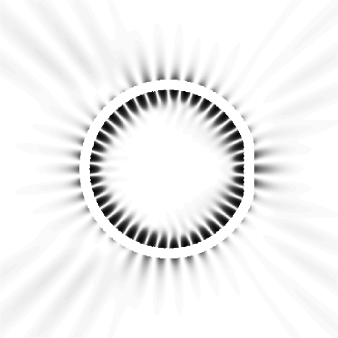
a)

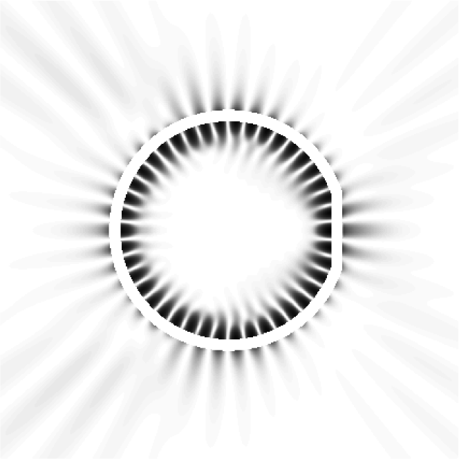
b)

Figure 7: a) Modulus square of the wave function for the cut disk with $\epsilon=.05$ obtained by direct numerical simulations corresponding to quasi-stationary eigen-momentum $kR=16.655-0.0199~{}{\rm i}$ b) The same but calculated within perturbation expansion with $m=21$ and $p=0$. The corresponding eigen-momentum is $kR=16.659-0.0191~{}{\rm i}$. The high intensity regions are indicated in black.

Finally, in Fig. 8, the far-field emission pattern computed numerically for the cut disk is compared with the same deduced from the perturbation series (48). The both are normalized to unit maximum. Once more a good agreement is found.

Figure 8: Far field emission pattern, $|F(\theta)|^{2}$, for the same state as in Fig. 7. Results from direct numerical simulations are plotted in solid black line, while the dashed red line indicates the perturbation result (48). The blue points correspond to experimental results with $\epsilon=0.05$ and $R=60~{}\mu$m.

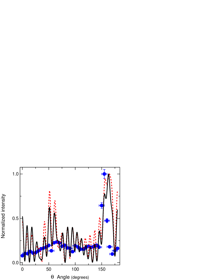
The approximate positions of the main peaks in the far-field pattern correspond to the diffracted rays emanated from the discontinuities of the cut disk boundaries and reflected at the critical angle (8) on the circular boundary (see Fig. 9).

Figure 9: Dashed and dotted lines: two main diffracted rays responsible for dominant peaks in the far-field pattern of a dielectric cut disk. All rays hit the circular boundary wi th an angle equal the critical angle (8).

If $(\theta_{1},\theta_{2},\ldots)$ and $(\theta_{1}^{\prime},\theta_{2}^{\prime},\ldots)$ are the directions of two such refracted rays one gets from geometrical considerations

$$\theta_{1} = \frac{\pi}{2}+2\theta_{c}-\theta_{m}\ ,\;\theta_{1}^{\prime}=\frac{3\pi}{2}-2\theta_{c}-\theta_{m}\ ,\;$$

$$\theta_{2} = 4\theta_{c}-\theta_{m}-\frac{\pi}{2}\ ,\;\theta_{2}^{\prime}=4\theta_{c}+\theta_{m}-\frac{\pi}{2}\ .$$ (88)

Here $\theta_{c}$ is the critical angle (8) and $\theta_{m}$ is defined in (87). For $\epsilon=.05$ and $n=1.5$, $\theta_{1}\approx 155.4^{\circ}$, $\theta_{1}^{\prime}\approx 168.2^{\circ}$, $\theta_{2}\approx 59^{\circ}$, and $\theta_{2}^{\prime}\approx 95.4^{\circ}$ which agrees with Fig. 8.

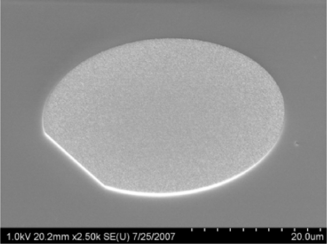
To complete this study, far-field experiments have been carried out according to the set-up described in apl . The cavities are made of a layer of polymethylmethacrylate (PMMA) doped by $4-dicyanomethylene-2-methyl-6-(4-dimethylaminostyryl)-4H-pyran$ (DCM, 5 % in weight) on a silica on silicon wafer. To obtain a good resolution of the shape even for such a small cut as $\epsilon=0.05$, cavities are defined with electron beam lithography (Leica EBPG 5000+) by C. Ulysse (Laboratoire de Photonique et de Nanostructures, CNRS-UPR20). A scanning electron microscope image of such a cavity is shown in Fig. 10.

Figure 10: Scanning electron microscope image of a cut disk etched with an electron beam.

As specified in apl , the cavities are uniformly pumped one by one from the top at 532 nm with a pulsed doubled Nd:YAG laser. The light emitted from the cavity is collected in its plane with a lens leading to a $10^{\circ}$ apex angle aperture. The directions of emission are symmetrical about the 0^∘ axis according to the obvious symmetry of the cut-disk shape. In Fig. 8, the intensity detected in the far-field is plotted versus the $\theta$ angle with blue points. The position of the maximal peak around $160^{\circ}$ is reproducible from cavity to cavity with $\epsilon=0.05$ and agrees with both numerical and perturbation approaches.

The example of the cut disk clearly demonstrates the usefulness of the perturbation method presented in this paper for deformed circular cavities.

VI Conclusion

We considered in details the construction of perturbation series for deformed dielectric circular cavities. The obtained formulae can be applied for the calculation of the spectrum and the wave functions as well as other characteristics of these dielectric cavities (e.g. far-field emission patterns). We checked these formulae on the example of the cut disk which is of interest from an experimental point of view. Cavities of other shapes (e.g. spiral spiral ) can be considered analogously. This method can also be used to calculate the influence of a small boundary roughness on the emission properties of circular cavities.

Appendix A Whispering gallery modes

The purpose of this Appendix is to calculate the asymptotic of quasi-stationary eigenvalues for a fixed radial quantum number $p$ and a large azimuthal quantum number $m\to\infty$.

These resonances are well confined, so let us first find the corresponding asymptotic expression for zeros of Bessel functions $J_{m}(x_{m})=0$. To achieve this task it is convenient to use Langer’s formulae (see e.g. bateman 7.13.4) which are valid with ${\cal O}(m^{-4/3})$ accuracy

$$J_{m}(x) = T(w)[J_{1/3}(z)\cos(\pi/6)-Y_{1/3}(z)\sin(\pi/6)]\ ,$$

$$Y_{m}(x) = T(w)[J_{1/3}(z)\cos(\pi/6)+Y_{1/3}(z)\sin(\pi/6)]\ ,$$

where $T(w)=w^{-1/2}(w-\arctan(w))^{1/2}$, $w=(x^{2}/m^{2}-1)^{1/2}$, and $z=m(w-\arctan(w))\;.$

The combination of the Bessel functions is expressed as follows

$$J_{1/3}(z)\cos(\pi/6)-Y_{1/3}(z)\sin(\pi/6)$$

$$=3^{1/6}2^{1/3}z^{-1/3}\textrm{ Ai}\Big{(}-\big{(}3z/2\big{)}^{2/3}\Big{)}$$ (89)

where $\textrm{ Ai}(x)$ is the Airy function

$$\textrm{ Ai}(x)=\frac{1}{\pi}\int_{0}^{\infty}\cos\big{(}\frac{t^{3}}{3}+tx\big{)}{\rm d}t\ .$$ (90)

Therefore in the intermediate region when $z$ is fixed and $m\gg 1$, the zeros of the $J_{m}$ Bessel function correspond to

$$z=\frac{2}{3}\eta_{p}^{3/2}$$ (91)

where $\eta_{p}$ are the modulus of the zeros of the Airy function Ai$(-\eta_{p})=0$ ($\eta_{1}\approx 2.338\;,\;\eta_{2}\approx 4.088\;,\;\eta_{3}\approx 5.521$). Finally, the Bessel function zeros have the following expansion

$$x_{m}=m+\alpha m^{1/3}+\beta m^{-1/3}+{\cal O}(m^{-1})$$ (92)

where

$$\alpha=2^{-1/3}\eta_{p}\;,\;\;\beta=\frac{3}{2^{5/3}5}\eta_{p}^{2}\ .$$ (93)

For $p=1$ this expression agrees numerically with the one given in bateman sect. 7.9.

The whispering gallery zeros of Bessel functions (92) permit to calculate explicitly the whispering gallery modes for the dielectric disk. Indeed we are interesting in the solutions of equation

$$\frac{n}{\nu}\frac{J_{m}^{\prime}}{J_{m}}(nx)=\frac{H_{m}^{(1)\prime}}{H_{m}}(x)$$ (94)

in the region $xn$ close to $m$, what means

$$xn=x_{m}+\delta x$$ (95)

with $\delta x\ll x_{m}$. The expansion of the right-hand side of Eq. (94) leads to

$$\frac{H_{m}^{(1)\prime}}{H_{m}}\big{(}\frac{x_{m}}{n}\big{)}=-\sqrt{n^{2}-1}+\frac{\alpha n^{2}}{m^{2/3}\sqrt{n^{2}-1}}+{\cal O}(m^{-1})\ .$$ (96)

In the left-hand side of Eq. (94), both numerator and denominator can be expanded into powers of $\delta x$ taking into account that $J_{m}(x_{m})=0$

$$\frac{J_{m}^{\prime}}{J_{m}}(x_{m}+\delta x)\approx\frac{J_{m}^{\prime}+\delta xJ_{m}^{\prime\prime}+(\delta x)^{2}J_{m}^{\prime\prime\prime}}{\delta xJ_{m}^{\prime}+(\delta x)^{2}J_{m}^{\prime\prime}/2+(\delta x)^{3}J_{m}^{\prime\prime\prime}/6}(x_{m})\ .$$ (97)

Using the Bessel equation

$$J_{m}^{\prime\prime}(z)+\frac{1}{z}J_{m}^{\prime}(z)+\left(1-\frac{m^{2}}{z^{2}}\right)J_{m}(z)=0$$ (98)

one can check that all but one derivatives $J_{m}^{(k)}/J_{m}^{\prime}(x_{m})$ are at most ${\cal O}(m^{-1})$ and can be neglected. The only exception is

$$\frac{J_{m}^{\prime\prime\prime}}{J_{m}^{\prime}}(x_{m})=-\frac{2\alpha}{m^{2/3}}+{\cal O}(m^{-1})\ .$$ (99)

Finally expansion (97) takes the form

$$\frac{J_{m}^{\prime}}{J_{m}}(x_{m}+\delta x)=\frac{1}{\delta x}-\delta x\frac{2\alpha}{3m^{2/3}}+{\cal O}(m^{-1})\ .$$ (100)

Combining this equation with (94) and (96) one obtains

$$\delta x=-\frac{n}{\nu\sqrt{n^{2}-1}}+\frac{\alpha n^{3}}{m^{2/3}\nu(n^{2}-1)^{3/2}}(\frac{2}{3\nu^{2}}-1)+{\cal O}(m^{-1}).$$ (101)

These formulae lead to Eq. (18).

Other ’whispering gallery’ modes correspond to $x$ close to $m$. With the same notations as above, Langer’s formula can be written for the Hankel function

$$H_{m}^{(1)}(x)=T(w){\rm e}^{{\rm i}\pi/6}H_{1/3}^{(1)}(z)+{\cal O}(m^{-4/3})\ .$$ (102)

The zeros of $H_{1/3}(z)$ exist only when $z=r{\rm e}^{-{\rm i}\pi}$ with real $r$. From formula bateman 7.11.42, it follows that

$$H_{\nu}^{(1)}(r{\rm e}^{{\rm i}m\pi}) = -\frac{\sin\pi(m-1)\nu}{\sin\pi\nu}H_{\nu}^{(1)}(r)+$$ (103)

$$+ {\rm e}^{-{\rm i}\pi\nu}\frac{\sin\pi m\nu}{\sin\pi\nu}H_{\nu}^{(2)}(r)\ .$$

In this way we get

$$H_{1/3}^{(1)}(r{\rm e}^{-{\rm i}\pi})=2{\rm e}^{-{\rm i}\pi/6}$$ (104)

$$\times \big{[}J_{1/3}(r)\cos(\pi/6)-Y_{1/3}(r)\sin(\pi/6)\big{]}\ .$$

This is the same combination of the Bessel functions as Eq. 89) for $J_{m}(x)$. Therefore the first complex zeros of the Hankel function, $H_{m}^{(1)}(\tilde{x}_{m})$, have a form similar to (92)

$$\tilde{x}_{m}=m+\tilde{\alpha}m^{1/3}+\tilde{\beta}m^{-1/3}+{\cal O}(m^{-1})$$ (105)

where $\tilde{\alpha}={\rm e}^{-2\pi{\rm i}/3}\alpha$ and $\tilde{\beta}={\rm e}^{-4\pi{\rm i}/3}\beta$ with the same $\alpha$ and $\beta$ as in (93).

The next step is to find the asymptotic of $J_{m}(nx)$ for complex $x=\tilde{x}_{m}$. As

$${\mbox{I}m}(\tilde{x}_{m})=-2^{-1/3}\sin(2\pi/3)\eta_{p}m^{1/3}+{\cal O}(m^{-1/3})\ ,$$ (106)

it tends to $-\infty$ with increasing of $m$. Therefore from (14) it follows that, instead of the $\cos(\ldots)$ term, only the positive exponent has to be taken into account. Then the left-hand side of (94) leads to

$$\frac{J_{m}^{\prime}}{J_{m}}(n\tilde{x}_{m})={\rm i}\sqrt{1-\frac{m^{2}}{n^{2}\tilde{x}_{m}^{2}}}+{\cal O}(m^{-1})$$

$$= {\rm i}\frac{\sqrt{n^{2}-1}}{n}\left(1+\frac{\tilde{\alpha}}{(n^{2}-1)m^{2/3}}\right)+{\cal O}(m^{-1})\ .$$

As $H_{m}^{(1)}(z)$ also obeys Eq. (98) one obtains the same expansion as (100)

$$\frac{H_{m}^{(1)\prime}}{H_{m}^{(1)}}(\tilde{x}_{m}+\delta x))=\frac{1}{\delta x}-\delta x\frac{2\tilde{\alpha}}{3m^{2/3}}+{\cal O}(m^{-1})\ .$$ (108)

Eqs. (A) and (108) lead to the following value of $\delta x$ with ${\cal O}(m^{-1})$ accuracy

$$\delta x=-\frac{{\rm i}\nu}{\sqrt{n^{2}-1}}+\frac{{\rm i}\nu\tilde{\alpha}}{m^{2/3}\sqrt{n^{2}-1}}\left(1-\frac{2\nu^{2}}{3}\right)\ .$$ (109)

Collecting these equations we get (19).

Appendix B Construction of perturbation series

From Eqs. (24) – (28), the following relations are valid at the circle $r=R$:

$$\Psi_{1}-\Psi_{2} = -\lambda^{2}\sum_{p}\gamma_{p}\cos(p\theta)+{\cal O}(\lambda^{3})\,$$

$$\frac{\partial\Psi_{1}}{\partial r}-\frac{\partial\Psi_{2}}{\partial r} = k\left[S_{m}(x)\cos(m\theta)\right.$$

$$+ \lambda\sum_{p\neq m}(\alpha_{p}+\lambda\beta_{p})S_{p}(x)\cos(p\theta)$$

$$+ \left.\lambda^{2}\sum_{p}\gamma_{p}\frac{H_{p}^{(1)\prime}}{H_{p}^{(1)}}(x)\cos(p\theta)\right]+{\cal O}(\lambda^{3})\;,$$

$$\frac{\partial^{2}\Psi_{1}}{\partial r^{2}}-\frac{\partial^{2}\Psi_{2}}{\partial r^{2}}=-\frac{k}{R}\left[(S_{m}(x)+x(n^{2}-1))\cos(m\theta)\right.$$

$$+\left.\lambda\sum_{p\neq m}\alpha_{p}(S_{p}(x)+x(n^{2}-1))\cos(p\theta)\right]+{\cal O}(\lambda^{2})\ ,$$

and

$$\frac{\partial^{3}\Psi_{1}}{\partial r^{3}}-\frac{\partial^{3}\Psi_{2}}{\partial r^{3}}=\left[kS_{m}(x)\left(\frac{m^{2}+2}{R^{2}}-k^{2}n^{2}\right)\right.$$

$$-k^{3}(n^{2}-1)\frac{H_{m}^{(1)\prime}}{H_{m}^{(1)}}(x)\left.+k^{2}\frac{n^{2}-1}{R}\right]\cos(m\theta)+{\cal O}(\lambda)\ .$$

In the zeroth order $S_{m}(x_{0})=0$. Expanding $S_{m}(x)$ with $x$ as in (30) into a series in $\lambda$, one gets

$$S_{m}(x_{0}+\lambda x_{1}+\lambda^{2}x_{2})=\lambda x_{1}\frac{\partial S_{m}}{\partial x}$$

$$+\lambda^{2}\left(x_{2}\frac{\partial S_{m}}{\partial x}+\frac{1}{2}x_{1}^{2}\frac{\partial^{2}S_{m}}{\partial x^{2}}\right)+{\cal O}(\lambda^{2})$$

where all derivatives of $S_{m}$ are taken at $x=x_{0}$. These derivatives are deduced from the Bessel equation (98)

$$\frac{\partial S_{m}}{\partial x}(x)=-(n^{2}-1)-\frac{1}{x}S_{m}(x)$$

$$-S_{m}(x)\left(S_{m}(x)+2\frac{H_{m}^{(1)\prime}}{H_{m}^{(1)}}(x)\right)\ .$$

In particular, when $x=x_{0}$

$$\frac{\partial S_{m}}{\partial x}(x_{0}) = -(n^{2}-1)$$ (110)

$$\frac{\partial^{2}S_{m}}{\partial x^{2}}(x_{0}) = (n^{2}-1)\left(\frac{1}{x_{0}}+2\frac{H_{m}^{(1)\prime}}{H_{m}^{(1)}}(x_{0})\right)\ .$$

In the $\lambda$ first order, it leads to

$$-x_{1}(n^{2}-1)\cos(m\theta)+\sum_{p\neq m}\alpha_{p}S_{p}(x_{0})\cos(p\theta)$$

$$=\frac{f(\theta)}{R}x_{0}(n^{2}-1)\cos(m\theta)\ .$$ (111)

Coefficients $\alpha_{p}$ and the first eigenvalue correction, $x_{1}$, are determined by comparison of the Fourier harmonics in both sides of Eq. (111)

$$\alpha_{p}=(n^{2}-1)\frac{x_{0}}{S_{p}(x_{0})}A_{pm}$$ (112)

and

$$x_{1}=-x_{0}A_{mm}$$ (113)

where $A_{pm}$ are the Fourier harmonics of the deformation function

$$A_{pm}=\frac{\epsilon_{p}}{\pi R}\int_{0}^{\pi}f(\theta)\cos(p\theta)\cos(m\theta){\rm d}\theta\ .$$ (114)

Here

$$\epsilon_{p}=\left\{\begin{array}[]{rl}2&\mbox{ for }p\neq 0\\ 1&\mbox{ for }p=0\end{array}\right.\ .$$ (115)

In the $\lambda$ second order, it leads to the following two equations

$$\sum_{p}\gamma_{p}\cos(p\theta)=\frac{1}{2}x_{0}^{2}(n^{2}-1)\frac{f^{2}(\theta)}{R^{2}}\cos(m\theta)$$ (116)

and

$$\left[(n^{2}-1)\Big{(}-x_{2}+\frac{1}{2x_{0}}x_{1}^{2}\Bigg{(}1+2x_{0}\frac{H_{m}^{(1)\prime}}{H_{m}^{(1)}}\Big{)}\Big{)}+\gamma_{m}\frac{H_{m}^{(1)\prime}}{H_{m}^{(1)}}\right]\cos(m\theta)$$

$$+\sum_{p\neq m}\left[x_{1}\alpha_{p}\frac{\partial S_{p}}{\partial x}+\beta_{p}S_{p}+\gamma_{p}\frac{H_{p}^{(1)\prime}}{H_{p}^{(1)}}\right]\cos(p\theta)$$ (117)

$$=\frac{f(\theta)}{R}\sum_{p\neq m}\alpha_{p}\Big{(}S_{p}+x_{0}(n^{2}-1)\Big{)}\cos(p\theta)-\frac{f^{2}(\theta)}{2R^{2}}x_{0}(n^{2}-1)\left(1-x_{0}\frac{H_{m}^{(1)\prime}}{H_{m}^{(1)}}\right)\cos(m\theta)\ .$$

Using (111) the right hand side of equation (117) can be rewritten as

$$(n^{2}-1)\frac{f(\theta)}{R}\left(x_{0}\sum_{p\neq m}\alpha_{p}\cos(p\theta)+x_{1}\cos(m\theta)\right)$$

$$+(n^{2}-1)\frac{f^{2}(\theta)}{2R^{2}}x_{0}\left(1+x_{0}\frac{H_{m}^{(1)\prime}}{H_{m}^{(1)}}\right)\cos(m\theta)\ .$$

Unknown coefficients can be determined by equating the Fourier harmonics in both parts of equations (116) and (117). From (116) it follows that for all $p$

$$\gamma_{p}=\frac{1}{2}x_{0}^{2}(n^{2}-1)B_{pm}\ .$$ (118)

where $B_{pm}$ represents the Fourier harmonics of the square of the deformation function

$$B_{pm}=\frac{\epsilon_{p}}{\pi R^{2}}\int_{0}^{\pi}f^{2}(\theta)\cos(p\theta)\cos(m\theta){\rm d}\theta\ .$$ (119)

For $p\neq m$ Eq. (117) gives

$$\beta_{p}S_{p}+x_{1}\alpha_{p}\frac{\partial S_{p}}{\partial x}+\gamma_{p}\frac{H_{p}^{(1)\prime}}{H_{p}^{(1)}}=(n^{2}-1)\Big{[}x_{1}A_{pm}$$

$$+x_{0}\sum_{k\neq m}\alpha_{k}A_{pk}+\frac{1}{2}x_{0}\Big{(}1+x_{0}\frac{H_{m}^{(1)\prime}}{H_{m}^{(1)}}\Big{)}B_{pm}\Big{]}\ .$$

The $m^{\mbox{th}}$ harmonic of the same equation determines the second correction to the quasi-stationary eigenvalue

$$x_{2}=\frac{1}{2x_{0}}x_{1}^{2}\Big{(}1+2x_{0}\frac{H_{m}^{(1)\prime}}{H_{m}^{(1)}}\Big{)}+\frac{\gamma_{m}H_{m}^{(1)\prime}}{(n^{2}-1)H_{m}^{(1)}}-$$

$$\frac{1}{2}x_{0}\Big{(}1+x_{0}\frac{H_{m}^{(1)\prime}}{H_{m}^{(1)}}\Big{)}B_{mm}-x_{0}\sum_{k\neq m}\alpha_{k}A_{mk}-x_{1}A_{mm}\ .$$

Rearranging these equations and using the first order results and Eq. (118), one gets

$$x_{2}=x_{0}\Bigg{[}\frac{1}{2}(3A_{mm}^{2}-B_{mm})$$ (120)

$$+x_{0}\frac{H_{m}^{(1)\prime}}{H_{m}^{(1)}}(A_{mm}^{2}-B_{mm})-\sum_{k\neq m}\alpha_{k}A_{m,k}\Bigg{]}\ ,$$

and

$$\beta_{p}=x_{0}\frac{n^{2}-1}{S_{p}}\Bigg{[}A_{pm}A_{mm}\Big{(}\frac{x_{0}}{S_{p}}\frac{\partial S_{p}}{\partial x}-1\Big{)}$$ (121)

$$+\frac{1}{2}B_{pm}\Bigg{(}1+x_{0}\Big{(}\frac{H_{m}^{(1)\prime}}{H_{m}^{(1)}}+\frac{H_{p}^{(1)\prime}}{H_{p}^{(1)}}\Big{)}\Bigg{)}+\sum_{k\neq m}\alpha_{k}A_{pk}\Bigg{]}\ .$$

Appendix C Green function for the dielectric circular cavity

The Green function of the dielectric Helmholtz equation for the circular cavity, $G(\vec{x},\vec{y}\,)$, is defined as the solution of the following equation

$$\left(\Delta_{\vec{x}}+n^{2}_{0}(\vec{x}\,)k^{2}\right)G(\vec{x},\vec{y}\,)=\delta(\vec{x}-\vec{y}\,)$$ (122)

where $n_{0}^{2}$ is the ’potential for the circular cavity defined in (51).

Let us first consider the case when the $\vec{y}$ source point is inside the circle. In this case, when the $\vec{x}$ point is inside the cavity, the advanced Green function has the form

$$G(\vec{x},\vec{y}\,) =\sum_{m=-\infty}^{\infty}A_{m}J_{m}(nkr){\rm e}^{{\rm i}m(\theta-\phi)}$$ (123)

$$+\frac{1}{4{\rm i}}H_{0}^{(1)}(kn|\vec{x}-\vec{y}\,|)$$

and when the $\vec{x}$ point is outside the circle

$$G(\vec{x},\vec{y}\,)=\sum_{m=-\infty}^{\infty}B_{m}H_{m}^{(1)}(kr){\rm e}^{{\rm i}m(\theta-\phi)}$$ (124)

Here and below we assume that points $\vec{x}$ and $\vec{y}$ have polar coordinates $(r,\theta)$ and $(\rho,\phi)$ respectively.

Constants $A_{m}$ and $B_{m}$ are calculated from the boundary conditions on the interface using the expansion bateman 7.15.29 of $H_{0}^{(1)}(k|\vec{x}-\vec{y}\,|)$

$$H_{0}^{(1)}(k|\vec{x}-\vec{y}\,|)=\sum_{m=-\infty}^{\infty}J_{m}(kr)H_{m}^{(1)}(k\rho){\rm e}^{{\rm i}m(\theta-\phi)}$$ (125)

when $r<\rho$ and

$$H_{0}^{(1)}(k|\vec{x}-\vec{y}\,|)=\sum_{m=-\infty}^{\infty}H_{m}^{(1)}(kr)J_{m}(k\rho){\rm e}^{{\rm i}m(\theta-\phi)}$$ (126)

when $r>\rho$.

For the TM polarization the Green function and its normal derivative at circle boundary are continuous. That leads to the following system of equations (with $x=kR$)

$$A_{m}J_{m}(nx)+\frac{1}{4{\rm i}}J_{m}(nk\rho)H_{m}^{(1)}(nx) = B_{m}H_{m}^{(1)}(x)$$

$$nA_{m}J_{m}^{\prime}(nx)+\frac{n}{4{\rm i}}J_{m}(nk\rho)H_{m}^{(1)\prime}(nx) = B_{m}H_{m}^{(1)\prime}(x)\ .$$

Its solutions are

$$A_{m} = -\frac{H_{m}^{(1)}(x)}{2\pi x\Delta_{m}J_{m}(nx)}J_{m}(kn\rho)-\frac{H_{m}^{(1)}(nx)}{4{\rm i}J_{m}(nx)}J_{m}(kn\rho),$$

$$B_{m} = -\frac{1}{2\pi x\Delta_{m}}J_{m}(kn\rho)\ .$$

where

$$\Delta_{m} = nJ_{m}^{\prime}(nx)H_{m}^{(1)}(x)-J_{m}(nx)H_{m}^{(1)\prime}(x)$$

$$\equiv J_{m}(nx)H_{m}^{(1)}(x)S_{m}(x)\ .$$

In deriving these expressions, the Wronskian (bateman 7.11.29) has been used

$$J_{\nu}(x)H_{\nu}^{(1)\prime}(x)-J_{\nu}^{\prime}(x)H_{\nu}^{(1)}(x)=\frac{2{\rm i}}{\pi x}\ .$$ (128)

For the $\vec{y}$ source point outside the circle, when $\vec{x}$ is inside the cavity, then

$$G(\vec{x},\vec{y}\,)=\sum_{m=-\infty}^{\infty}C_{m}J_{m}(nkr){\rm e}^{{\rm i}m(\theta-\phi)}$$ (129)

and when $\vec{x}$ is outside the circle, then

$$G(\vec{x},\vec{y}\,) = \sum_{m=-\infty}^{\infty}D_{m}H_{m}^{(1)}(kr){\rm e}^{{\rm i}m(\theta-\phi)}$$

$$+ \frac{1}{4{\rm i}}H_{0}^{(1)}(k|\vec{x}-\vec{y}\,|)\ .$$

Constants $C_{m}$ and $D_{m}$ are computed exactly as $A_{m}$ and $B_{m}$:

$$C_{m} = -\frac{1}{2\pi x\Delta_{m}}H_{m}^{(1)}(k\rho)\ ,$$

$$D_{m} = -\frac{J_{m}(nx)}{2\pi x\Delta_{m}H_{m}^{(1)}(x)}H_{m}^{(1)}(k\rho)-\frac{J_{m}(x)}{4{\rm i}H_{m}(x)}H_{m}^{(1)}(k\rho)\ .$$

The final expressions of the Green function follow from the above formulae.

When the $\vec{y}$ source point is inside the circle, the plane is divided into three parts: 1) $r<\rho$, 2) $\rho<r<R$, 3) $R<r$. Denoting the Green function in these regions by the corresponding numbers, it can be written as

$$G_{j}(\vec{x},\vec{y}\,)=\sum_{p=0}^{\infty}g_{p}^{(j)}(r,\rho)\cos[p(\theta-\phi)]$$ (131)

where

$$g_{p}^{(1)}(r,\rho)=-\frac{1}{2\pi x}\epsilon_{p}\frac{J_{p}(nkr)J_{p}(nk\rho)}{J_{p}^{2}(nx)S_{p}(x)}$$

$$+\frac{1}{4{\rm i}}\epsilon_{p}\frac{J_{p}(knr)}{J_{p}(nx)}[H_{p}^{(1)}(kn\rho)J_{p}(nx)-H_{p}^{(1)}(nx)J_{p}(kn\rho)],$$

$$g_{p}^{(2)}(r,\rho)=-\frac{1}{2\pi x}\epsilon_{p}\frac{J_{p}(nkr)J_{p}(nk\rho)}{J_{p}^{2}(nx)S_{p}(x)}$$

$$+\frac{1}{4{\rm i}}\epsilon_{p}\frac{J_{p}(kn\rho)}{J_{p}(nx)}[H_{p}^{(1)}(knr)J_{p}(nx)-H_{p}^{(1)}(nx)J_{p}(knr)],$$

$$g_{p}^{(3)}(r,\rho)=-\frac{1}{2\pi x}\epsilon_{p}\frac{J_{p}(nk\rho)H_{p}^{(1)}(kr)}{J_{p}(nx)H_{p}^{(1)}(x)S_{p}(x)}$$

where $\epsilon_{p}$ was defined in (115).

When point $\vec{y}$ is outside the circle, the plane is divided into three different regions 1) $r<R$, 2) $R<r<\rho$, 3) $\rho<r$. With the same notation as above, the Green function can be written

$$\tilde{G}_{j}(\vec{x},\vec{y}\,)=\sum_{p=0}^{\infty}\tilde{g}_{p}^{(j)}(r,\rho)\cos[p(\theta-\phi)]$$ (132)

where

$$\tilde{g}_{p}^{(1)}(r,\rho)=-\frac{1}{2\pi x}\epsilon_{p}\frac{J_{p}(nkr)H_{p}^{(1)}(k\rho)}{J_{p}(nx)H_{p}^{(1)}(x)S_{p}(x)}\ ,$$

$$\tilde{g}_{p}^{(2)}(r,\rho)=-\frac{1}{2\pi x}\epsilon_{p}\frac{H_{p}^{(1)}(kr)H_{p}^{(1)}(k\rho)}{H_{p}^{(1)2}(x)S_{p}(x)}$$

$$+\frac{1}{4{\rm i}}\epsilon_{p}\frac{H_{p}^{(1)}(k\rho)}{H_{p}^{(1)}(x)}[H_{p}^{(1)}(x)J_{p}(kr)-H_{p}^{(1)}(kr)J_{p}(x)]\ ,$$

$$\tilde{g}_{p}^{(3)}(r,\rho)=-\frac{1}{2\pi x}\epsilon_{p}\frac{H_{p}^{(1)}(kr)H_{p}^{(1)}(k\rho)}{H_{p}^{(1)2}(x)S_{p}(x)}$$

$$+\frac{1}{4{\rm i}}\epsilon_{p}\frac{H_{p}^{(1)}(kr)}{H_{p}^{(1)}(x)}[H_{p}^{(1)}(x)J_{p}(k\rho)-H_{p}^{(1)}(k\rho)J_{p}(x)]\ .$$

Notice that $G_{1}(\vec{x},\vec{y}\,)=G_{2}(\vec{y},\vec{x}\,)$, $G_{3}(\vec{x},\vec{y}\,)=\tilde{G}_{1}(\vec{y},\vec{x}\,)$, and $\tilde{G}_{2}(\vec{x},\vec{y}\,)=\tilde{G}_{3}(\vec{y},\vec{x}\,)$. It means that in all cases the Green function is symmetric: $G(\vec{x},\vec{y}\,)=G(\vec{y},\vec{x}\,)$ as it should be (see e.g. morse ).

Appendix D Three degenerate levels

For three quasi-degenerate levels, instead of Eq. (84) one gets the $3\times 3$ determinant

$$\left|\begin{array}[]{ccc}\delta x-s_{1}&A_{12}&A_{13}\\ A_{21}&\delta x-s_{2}&A_{23}\\ A_{31}&A_{32}&\delta x-s_{3}\end{array}\right|=0$$ (133)

which leads to the cubic equation

$$(\delta x)^{3}-\sigma_{1}(\delta x)^{2}+(\sigma_{2}-\alpha)\delta x-\sigma_{3}+\beta=0\ .$$ (134)

Here $\sigma_{i}$ are the elementary symmetric functions of $s_{i}$

$$\sigma_{1}=s_{1}+s_{2}+s_{3}\ ,\;\sigma_{2}=s_{1}s_{2}+s_{2}s_{3}+s_{3}s_{1}\ ,\;\sigma_{3}=s_{1}s_{2}s_{3}\ .$$

and (because $A_{ij}=A_{ji}$)

$$\alpha = A_{12}^{2}+A_{23}^{2}+A_{31}^{2}\ ,$$

$$\beta = 2A_{12}A_{23}A_{31}+s_{1}A_{23}^{2}+s_{2}A_{31}^{2}+s_{3}A_{12}^{2}\ .$$

To solve Eq. (134), the next steps are standard. The substitution

$$\delta x=y+\frac{1}{3}\sigma_{1}$$ (135)

transforms Eq. (134) to the reduced form

$$y^{3}+py+q=0$$ (136)

where

$$p=-\frac{1}{3}\sigma_{1}^{2}+\sigma_{2}-\alpha\ ,\;q=-\frac{2}{27}\sigma_{1}^{3}+\frac{1}{3}\sigma_{1}\sigma_{2}-\sigma_{3}+\delta\ .$$ (137)

with $\delta=\beta-\frac{1}{3}\sigma_{1}\alpha$. Finally after the transformation

$$y=z-\frac{p}{3z}$$ (138)

one gets the equation $z^{3}-\frac{p^{3}}{27z^{3}}+q=0$ which is a quadratic equation in variable

$$w=z^{3}\;.$$ (139)

Its solution is

$$w=-\frac{q}{2}\pm\sqrt{\frac{q^{2}}{4}+\frac{p^{3}}{27}}\ .$$ (140)

Eqs. (135), (138), (139), and (140) give the well known solution of the cubic equation (134). The question is how to choose a branch which tends to $s_{1}$ when $A_{ij}\to 0$. The discriminant of this equation is

$$D\equiv\frac{q^{2}}{4}+\frac{p^{3}}{27}=d+\varepsilon$$ (141)

where

$$d=\frac{1}{4}\Big{(}-\frac{2}{27}\sigma_{1}^{3}+\frac{1}{3}\sigma_{1}\sigma_{2}-\sigma_{3}\Big{)}^{2}+\frac{1}{27}\Big{(}\sigma_{2}-\frac{1}{3}\sigma_{1}^{2}\Big{)}^{3}$$

and

$$\varepsilon = \frac{1}{4}\delta^{2}+\frac{1}{2}\delta\Big{(}-\frac{2}{27}\sigma_{1}^{3}+\frac{1}{3}\sigma_{1}\sigma_{2}-\sigma_{3}\Big{)}$$

$$- \frac{1}{27}\alpha^{3}+\frac{1}{9}\alpha^{2}(\sigma_{2}-\frac{1}{3}\sigma_{1}^{2})-\frac{1}{9}\alpha(\sigma_{2}-\frac{1}{3}\sigma_{1}^{2})^{2}\ .$$

Using the identity

$$d=-\frac{1}{108}\Big{[}(s_{1}-s_{2})(s_{2}-s_{3})(s_{3}-s_{1})\Big{]}^{2}$$

the expression (140) can be transformed into

$$w = w_{0}-\frac{1}{2}\delta+\frac{{\rm i}}{6\sqrt{3}}(s_{1}-s_{2})(s_{2}-s_{3})(s_{3}-s_{1})$$

$$\times \left[\sqrt{1-\frac{108\varepsilon}{[(s_{1}-s_{2})(s_{2}-s_{3})(s_{3}-s_{1})]^{2}}}-1\right]$$

where

$$w_{0} = \frac{1}{27}\sigma_{1}^{3}-\frac{1}{6}\sigma_{1}\sigma_{2}+\frac{1}{2}\sigma_{3}$$

$$+ \frac{{\rm i}}{6\sqrt{3}}(s_{1}-s_{2})(s_{2}-s_{3})(s_{3}-s_{1})$$

$$= \frac{1}{27}\Big{(}s_{1}+s_{2}{\rm e}^{-2\pi{\rm i}/3}+s_{3}{\rm e}^{2\pi{\rm i}/3}\Big{)}^{3}\ .$$

Finally the root of the cubic equation (134) which tends to $s_{1}$ when $A_{ij}\to 0$ is

$$z=\frac{1}{3}s\left[1-\frac{27\delta}{2s^{3}}+\frac{3\sqrt{3}{\rm i}}{2s^{3}}(s_{1}-s_{2})(s_{2}-s_{3})(s_{3}-s_{1})\right.$$

$$\times\left.\Big{[}\sqrt{1-\frac{108\varepsilon}{[(s_{1}-s_{2})(s_{2}-s_{3})(s_{3}-s_{1})]^{2}}}-1\Big{]}\right]^{1/3}$$

where $s=s_{1}+s_{2}{\rm e}^{-2\pi{\rm i}/3}+s_{3}{\rm e}^{2\pi{\rm i}/3}$.

References

- (1) Optical microcavities, edited by K. Vahala (World Scientific, Singapore, 2005).
- (2) E. Krioukov, D.J. W. Klunder, A. Driessen, J. Greve, and C. Otto, Opt. Lett. 27, 512 (2002).
- (3) C. Gmachl, F. Capasso, E. E. Narimanov, J. U. Nöckel, A. D. Stone, J. Faist, D. L. Sivco, and A. Y. Cho, Science 280, 1556 (1998).
- (4) J.D. Jackson, Classical electrodynamics (John Wiley & Sons Inc., New York, London 1962).
- (5) C. Vassallo, Optical waveguide concepts (Eslevier, Amsterdam, 1991).
- (6) M. Lebental, N. Djellali, C. Arnaud, J.-S. Lauret, J. Zyss, R. Dubertrand, C. Schmit, and E. Bogomolny, to be published in Phys. Rev. A.
- (7) Erdélyi A, Higher Transcendental Functions, vol. 3 (Mc Graw-Hill, New York, Toronto, London, 1955)
- (8) J. Nöckel, PhD dissertation, Yale University, 1997.
- (9) M. Hentschel and H. Schomerus, Phys. Rev. E 65, 045603 (2002)
- (10) C. Yeh, Phys. Rev. 135, A1193 (1964).
- (11) L. Kaminetzky and J. Keller, SIAM J. Appl. Math. 22, 109 (1972).
- (12) I. Braun, G. Ihlein, F. Laeri, J.U. Nöckel, G. Schulz-Ekloff, F. Schüth, U. Vietze, O. Weis, D. Wöhrle, Appl. Phys. B 70, 335 (2000).
- (13) J. Wiersig, Journal of Applied Optics: pure and applied optics, 5, 53 (2003) ; J. Wiersig, Phys. Rev. A 67, 023807 (2003).
- (14) P.M. Morse and H. Feshbach, Methods of theoretical physics, v. II (McGraw-Hill, New York, Toronto, London, 1953).
- (15) M.V. Berry and M. Tabor, Proc. R. Soc. Lond. A 356, 375 (1977).
- (16) S. Tomsovic and D. Ullmo, Phys. Rev. E 50, 145 (1994).
- (17) V. Doya, O. Legrand, F. Mortessagne, and C. Miniatura, Phys. Rev. E 65, 056223 (2002).
- (18) M. Lebental, J.-S. Lauret, R. Hierle, J. Zyss, Applied Physics Letters, 88, 031108 (2006).
- (19) S.-Y. Lee, S. Rim, J.-W. Ryu, T.-Y. Kwon, and C.-M. Kim, Phys. Rev. Lett. 93, 164102 (2004).