The Isoconditioning Loci of Planar Three-DOF Parallel Manipulators

Abstract

The subject of this paper is a special class of three-degree-of-freedom parallel manipulators. The singular configurations of the two Jacobian matrices are first studied. The isotropic configurations are then found based on the characteristic length of this manipulator. The isoconditioning loci for the Jacobian matrices are plotted to define a global performance index allowing the comparison of the different working modes. The index thus resulting is compared with the Cartesian workspace surface and the average of the condition number.

1 Introduction

Various performance indices have been devised to assess the kinetostatic performances of serial and parallel manipulators. The literature on performance indices is extremely rich to fit in the limits of this paper, the interested reader being invited to look at it in the references cited here. A dimensionless quality index was recently introduced in [1] based on the ratio of the Jacobian determinant to its maximum absolute value, as applicable to parallel manipulators. This index does not take into account the location of the operation point of the end-effector, because the Jacobian determinant is independent of this location. The proof of the foregoing result is available in [2], as pertaining to serial manipulators, its extension to their parallel counterparts being straightforward. The condition number of a given matrix, on the other hand, is well known to provide a measure of invertibility of the matrix [3]. It is thus natural that this concept found its way in this context. Indeed, the condition number of the Jacobian matrix was proposed in [4] as a figure of merit to minimize when designing manipulators for maximum accuracy. In fact, the condition number gives, for a square matrix, a measure of the relative roundoff-error amplification of the computed results [3] with respect to the data roundoff error. As is well known, however, the dimensional inhomogeneity of the entries of the Jacobian matrix prevents the straightforward application of the condition number as a measure of Jacobian invertibility. The characteristic length was introduced in [5] to cope with the above-mentioned inhomogeneity.

In this paper we use the characteristic length to normalize the Jacobian matrix of a three-dof planar manipulator and to calculate the isoconditioning loci for all its working modes.

2 Preliminaries

A planar three-dof manipulator with three parallel PRR chains, the object of this paper, is shown in Fig. 1. This manipulator has been frequently studied, in particular in [6, 7]. The actuated joint variables are the displacements of the three prismatic joints, the Cartesian variables being the position vector p of the operation point $P$ and the orientation $\theta$ of the platform.

Figure 1: A three-DOF parallel manipulator

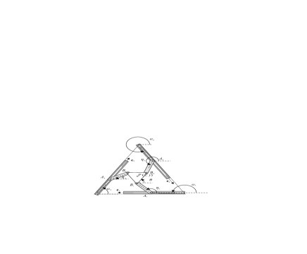
The trajectories of the points $A_{i}$ define an equilateral triangle whose geometric center is the point $O$, while the points $B_{1}$, $B_{2}$ and $B_{3}$, whose geometric center is the point $P$, lie at the corners of an equilateral triangle. We thus have $\alpha_{i}=\pi+(i-1)(2\pi/3)$, for $i=1,2,3$. Moreover, $l=l_{1}=l_{2}=l_{3}$, with $l_{i}$ denoting the length of $A_{i}B_{i}$ and $r=r_{1}=r_{2}=r_{3}$, with $r_{i}$ denoting the length of $B_{i}P$, in units of length that need not be specified in the paper. The layout of the trajectories of points $A_{i}$ is defined by the radius $R$ of the circle inscribed in the associated triangle.

2.1 Kinematic Relations

The velocity $\dot{\bf p}$ of point $P$ can be obtained in three different forms, depending on which leg is traversed, namely,

$$\dot{{\bf{p}}}=\dot{{\bf{a}}}_{1}+\dot{\eta}_{1}{\bf{E}}({\bf{b}}_{1}-{\bf{a}}_{1})+\dot{\theta}{\bf{E}}({\bf{p}}-{\bf{b}}_{1})$$ (1a)

$$\dot{{\bf{p}}}=\dot{{\bf{a}}}_{2}+\dot{\eta}_{2}{\bf{E}}({\bf{b}}_{2}-{\bf{a}}_{2})+\dot{\theta}{\bf{E}}({\bf{p}}-{\bf{b}}_{2})$$ (1b)

$$\dot{{\bf{p}}}=\dot{{\bf{a}}}_{3}+\dot{\eta}_{3}{\bf{E}}({\bf{b}}_{3}-{\bf{a}}_{3})+\dot{\theta}{\bf{E}}({\bf{p}}-{\bf{b}}_{3})$$ (1c)

with matrix ${\bf{E}}$ defined as

$${\bf E}=\left[\begin{array}[]{cr}0&~{}-1\\ 1&0\end{array}\right]$$

The velocity $\dot{{\bf{a}}_{i}}$ of points $A_{i}$ is given by

$$\dot{{\bf{a}}}_{i}=\dot{\rho}_{i}\frac{{\boldsymbol{\rho}}_{i}}{||{\boldsymbol{\rho}}_{i}||}=\dot{\rho}_{i}\left[\begin{array}[]{c}\cos(\alpha_{i})\\ \sin(\alpha_{i})\end{array}\right]=\dot{\rho}_{i}{\bf{e}}_{i}$$

where ${\bf{e}}_{i}$ is a unit vector in the direction of the $i$th prismatic joint.

We would like to eliminate the three idle joint rates $\dot{\eta}_{1}$, $\dot{\eta}_{2}$ and $\dot{\eta}_{3}$ from eqs.(1a-c), which we do upon dot-multiplying the former by $({\bf{b}}_{i}-{\bf{a}}_{i})^{T}$, thus obtaining

$$({\bf{b}}_{1}-{\bf{a}}_{1})^{T}\dot{{\bf{p}}}=({\bf{b}}_{1}-{\bf{a}}_{1})^{T}\dot{\rho}_{1}{\bf{e}}_{1}+({\bf{b}}_{1}-{\bf{a}}_{1})^{T}\dot{\theta}{\bf{E}}({\bf{p}}-{\bf{b}}_{1})$$ (2a)

$$({\bf{b}}_{2}-{\bf{a}}_{2})^{T}\dot{{\bf{p}}}=({\bf{b}}_{2}-{\bf{a}}_{2})^{T}\dot{\rho}_{2}{\bf{e}}_{2}+({\bf{b}}_{2}-{\bf{a}}_{2})^{T}\dot{\theta}{\bf{E}}({\bf{p}}-{\bf{b}}_{2})$$ (2b)

$$({\bf{b}}_{3}-{\bf{a}}_{3})^{T}\dot{{\bf{p}}}=({\bf{b}}_{3}-{\bf{a}}_{3})^{T}\dot{\rho}_{3}{\bf{e}}_{3}+({\bf{b}}_{3}-{\bf{a}}_{3})^{T}\dot{\theta}{\bf{E}}({\bf{p}}-{\bf{b}}_{3})$$ (2c)

Equations (2a-c) can now be cast in vector form, namely,

$${\bf A}{{\bf{t}}}={\bf B\dot{\boldsymbol{\rho}}}\quad{\rm with}\quad{\bf{t}}=\left[\begin{array}[]{c}\dot{{\bf{p}}}\\ \dot{\theta}\end{array}\right]\quad{\rm and}\quad\dot{\boldsymbol{\rho}}=\left[\begin{array}[]{c}\dot{\rho}_{1}\\ \dot{\rho}_{2}\\ \dot{\rho}_{3}\end{array}\right]$$ (3)

with $\dot{\boldsymbol{\rho}}$ thus being the vector of actuated joint rates.

Moreover, A and B are, respectively, the direct-kinematics and the inverse-kinematics matrices of the manipulator, defined as

$${\bf{A}} = \left[\begin{array}[]{cc}({\bf{b}}_{1}-{\bf{a}}_{1})^{T}&~{}~{}-({\bf{b}}_{1}-{\bf{a}}_{1})^{T}{\bf{E}}({\bf{p}}-{\bf{b}}_{1})\\ ({\bf{b}}_{2}-{\bf{a}}_{2})^{T}&~{}~{}-({\bf{b}}_{2}-{\bf{a}}_{2})^{T}{\bf{E}}({\bf{p}}-{\bf{b}}_{2})\\ ({\bf{b}}_{3}-{\bf{a}}_{3})^{T}&~{}~{}-({\bf{b}}_{3}-{\bf{a}}_{3})^{T}{\bf{E}}({\bf{p}}-{\bf{b}}_{3})\end{array}\right]$$ (4d)

$${\bf{B}} = \left[\begin{array}[]{ccc}({\bf{b}}_{1}-{\bf{a}}_{1})^{T}{\bf{e}}_{1}&0&0\\ 0&({\bf{b}}_{2}-{\bf{a}}_{2})^{T}{\bf{e}}_{2}&0\\ 0&0&({\bf{b}}_{3}-{\bf{a}}_{3})^{T}{\bf{e}}_{3}\end{array}\right]$$ (4h)

When A and B are nonsingular, we obtain the relations

$${\bf{t}}={\bf{J}}\dot{\boldsymbol{\rho}}{\rm,~{}~{}with~{}~{}}{\bf{J}}={\bf{A}}^{-1}{\bf{B}}\quad{\rm and}\quad\dot{\boldsymbol{\rho}}={\bf{K}}{\bf{t}}$$

with K denoting the inverse of J.

2.2 Parallel Singularities

Parallel singularities occur when the determinant of matrix A vanishes [8, 9]. At these configurations, it is possible to move locally the operation point $P$ with the actuators locked, the structure thus resulting cannot resist arbitrary forces, and control is lost. To avoid any performance deterioration, it is necessary to have a Cartesian workspace free of parallel singularities. For the planar manipulator studied, such configurations are reached whenever the axes $A_{1}B_{1}$, $A_{2}B_{2}$ and $A_{3}B_{3}$ intersect (possibly at infinity), as depicted in Fig. 3.

Figure 2: Parallel singularity

Figure 3: Serial singularity

In the presence of such configurations, moreover, the manipulator cannot resist a force applied at the intersection point. These configurations are located inside the Cartesian workspace and form the boundaries of the joint workspace [8].

2.3 Serial Singularities

Serial singularities occur when $\det({\bf{B}})=0$. In the presence of theses singularities, there is a direction along which no Cartesian velocity can be produced. Serial singularities define the boundary of the Cartesian workspace. For the topology under study, the serial singularities occur whenever $({\bf{b}}_{i}-{\bf{a}}_{i})^{T}{\bf{e}}_{i}=0$ for at least one value of $i$, as depicted in Fig. 3 for $i=2$.

3 Isoconditioning Loci

3.1 The Matrix Condition Number

We derive below the loci of equal condition number of the matrices A, B and K. To do this, we first recall the definition of condition number of an $m\times n$ matrix ${\bf{M}}$, with $m\leq n$, $\kappa({\bf{M}})$. This number can be defined in various ways; for our purposes, we define $\kappa({\bf{M}})$ as the ratio of the smallest, $\sigma_{s}$, to the largest, $\sigma_{l}$, singular values of ${\bf{M}}$, namely,

$$\kappa({\bf{M}})=\frac{\sigma_{s}}{\sigma_{l}}$$ (5)

The singular values $\left\{\sigma_{i}\right\}_{1}^{m}$ of matrix ${\bf{M}}$ are defined, in turn, as the square roots of the nonnegative eigenvalues of the positive-definite $m\times m$ matrix ${\bf{M}}{\bf{M}}^{T}$.

3.2 Non-Homogeneous Direct-Kinematics Matrix

To render the matrix ${\bf{A}}$ homogeneous, as needed to define its condition number, each term of the third column of ${\bf{A}}$ is divided by the characteristic length $L$ [10], thereby deriving its normalized counterpart $\overline{{\bf{A}}}$:

$$\overline{{\bf{A}}}=\left[\begin{array}[]{cc}({\bf{b}}_{1}-{\bf{a}}_{1})^{T}&~{}~{}-({\bf{b}}_{1}-{\bf{a}}_{1})^{T}{\bf{E}}({\bf{p}}-{\bf{b}}_{1})/L\\ ({\bf{b}}_{2}-{\bf{a}}_{2})^{T}&~{}~{}-({\bf{b}}_{2}-{\bf{a}}_{2})^{T}{\bf{E}}({\bf{p}}-{\bf{b}}_{2})/L\\ ({\bf{b}}_{3}-{\bf{a}}_{3})^{T}&~{}~{}-({\bf{b}}_{3}-{\bf{a}}_{3})^{T}{\bf{E}}({\bf{p}}-{\bf{b}}_{3})/L\end{array}\right]$$ (6)

which is calculated so as to minimize $\kappa(\overline{{\bf{A}}})$, along with the posture variables $\rho_{1}$, $\rho_{2}$ and $\rho_{3}$.

However, notice that B is dimensionally homogeneous, and need not be normalized.

3.3 Isotropic Configuration

In this section, we derive the isotropy condition on J to define the geometric parameters of the manipulator. We shall obtain also the value $L$ of the characteristic length. To simplify $\overline{{\bf{A}}}$ and B, we use the notation

$${\bf{l}}_{i} = ({\bf{b}}_{i}-{\bf{a}}_{i})$$ (7a)

$$k_{i} = ({\bf{b}}_{i}-{\bf{a}}_{i})^{T}{\bf{E}}({\bf{p}}-{\bf{b}}_{i})$$ (7b)

$$m_{i} = ({\bf{b}}_{i}-{\bf{a}}_{i})^{T}{\bf{e}}_{i}$$ (7c)

$$\gamma_{i} = \angle A_{i}B_{i}P$$ (7d)

We can thus write matrices $\overline{{\bf{A}}}$ and ${\bf{B}}$ as

$$\overline{{\bf{A}}}=\left[\begin{array}[]{cc}{\bf{l}}_{1}^{T}&-k_{1}/L\\ {\bf{l}}_{2}^{T}&-k_{2}/L\\ {\bf{l}}_{3}^{T}&-k_{3}/L\end{array}\right]\quad{\bf{B}}=\left[\begin{array}[]{ccc}m_{1}&0&0\\ 0&m_{2}&0\\ 0&0&m_{3}\end{array}\right]$$ (14)

Whenever matrix B is nonsingular, that is, when $m_{i}\neq 0$, for $i=1,2,3$, we have

$$\overline{{\bf{K}}}=\left[\begin{array}[]{ccc}{\bf{l}}_{1}^{T}/m_{1}&~{}~{}-k_{1}/(L~{}m_{1})\\ {\bf{l}}_{2}^{T}/m_{2}&~{}~{}-k_{2}/(L~{}m_{1})\\ {\bf{l}}_{3}^{T}/m_{3}&~{}~{}-k_{3}/(L~{}m_{3})\end{array}\right]$$

Matrix $\overline{{\bf{J}}}$, the normalized J, is isotropic if and only if $\overline{{\bf{K}}}\overline{{\bf{K}}}^{T}=\tau^{2}~{}{\bf{1}}_{3\times 3}$ for $\tau>0$ and $\overline{{\bf{K}}}=\overline{{\bf{J}}}^{-1}$, i.e.,

$$({\bf{l}}_{1}^{T}{\bf{l}}_{1}+k_{1}^{2}/L^{2})/m_{1}^{2}=\tau^{2}$$ (15a)

$$({\bf{l}}_{2}^{T}{\bf{l}}_{2}+k_{2}^{2}/L^{2})/m_{2}^{2}=\tau^{2}$$ (15b)

$$({\bf{l}}_{3}^{T}{\bf{l}}_{3}+k_{3}^{2}/L^{2})/m_{3}^{2}=\tau^{2}$$ (15c)

$$({\bf{l}}_{1}^{T}{\bf{l}}_{2}+k_{1}k_{2}/L^{2})/(m_{1}m_{2})=0$$ (15d)

$$({\bf{l}}_{1}^{T}{\bf{l}}_{3}+k_{1}k_{3}/L^{2})/(m_{1}m_{3})=0$$ (15e)

$$({\bf{l}}_{2}^{T}{\bf{l}}_{3}+k_{2}k_{3}/L^{2})/(m_{2}m_{3})=0$$ (15f)

From eqs.(15a-f), we can derive the conditions below:

$$||{\bf{l}}_{1}||=||{\bf{l}}_{2}||=||{\bf{l}}_{3}||$$ (16a)

$$||{\bf{p}}-{\bf{b}}_{1}||=||{\bf{p}}-{\bf{b}}_{2}||=||{\bf{p}}-{\bf{b}}_{3}||$$ (16b)

$${\bf{l}}_{1}^{T}{\bf{l}}_{2}={\bf{l}}_{2}^{T}{\bf{l}}_{3}={\bf{l}}_{2}^{T}{\bf{l}}_{3}$$ (16c)

$$m_{1}m_{2}=m_{1}m_{3}=m_{2}m_{3}$$ (16d)

In summary, the constraints defined in the eqs.(16a-d) are:

$\circ$

Pivots $B_{i}$ should be placed at the vertices of an equilateral triangle;

$\circ$

Segments $A_{i}B_{i}$ form an equilateral triangle;

$\circ$

The trajectories of point $A_{i}$ define an equilateral triangle an hence, $l=l_{1}=l_{2}=l_{3}$.

Notice that the foregoing conditions, except the second one, were assumed in $\S 2$.

3.4 The Characteristic Length

The characteristic length is defined at the isotropic configuration. From eqs.(15d-f), we determine the value of the characteristic length as,

$$L=\sqrt{\frac{-k_{1}k_{2}}{{\bf{l}}_{1}^{T}{\bf{l}}_{2}}}$$

By applying the constraints defined in eqs.(15a-d), we can write the characteristic length $L$ in terms of angle $\gamma$, i.e.

$$L=\sqrt{2}r\sin(\gamma)$$

where $\gamma=\gamma_{1}=\gamma_{2}=\gamma_{3}$, was defined in eq.(7d) and $\gamma\in[0~{}2\pi]$.

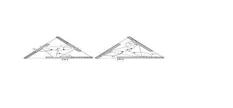
This means that the manipulator under study admits several isotropic configurations, two of which are shown in Figs. 4a and b, whereas the characteristic length $L$ of a manipulator is unique [2]. When $\gamma$ is equal to $\pi/2$, Fig. 4a, i.e., when $A_{i}B_{i}$ is perpendicular to $B_{i}P$, the manipulator finds itself at a configuration furthest away from parallel singularities. To have an isotropic configuration furthest away from serial singularities, we have two conditions: ${\bf{e}}_{i}^{T}{\bf{E}}({\bf{b}}_{i}-{\bf{a}}_{i})=0$ and $r=R/2$.

Figure 4: Two isotropic configurations with two values of $\rho$

3.5 Working Modes

The manipulator under study has a diagonal inverse-kinematics matrix B, as shown in eq.(5b), the vanishing of one of its diagonal entries thus indicating the occurrence of a serial singularity. The set of manipulator postures free of this kind of singularity is termed a working mode. The different working modes are thus separated by a serial singularity, with a set of postures in different working modes corresponding to an inverse kinematics solution.

The formal definition of the working mode is detailed in [8]. For the manipulator at hand, there are eight working modes, as depicted in Fig. 5.

Figure 5: The eight working modes of the $3PRR$ manipulator

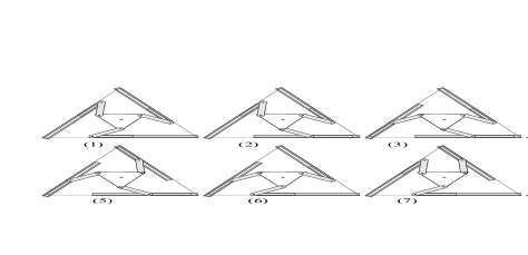
However, because of symmetries, we can restrict our study to only two working modes, if there are no joint limits. Indeed, working mode $1$ is similar to working mode $5$, because for the first one, the signs of the diagonal entries of ${\bf{B}}$ are all negative, and for the second are all positive. A similary reasoning is applicable to the working modes $2$-$6$, $3$-$7$ and $4$-$8$; likewise, the working modes $3$-$4$ and $7$-$8$ can be derived from the working modes 2 and 6 by a rotation of $120^{\circ}$ and $240^{\circ}$, respectively. Therefore, only the working modes $1$ and $2$ are studied. We label the corresponding matrices as $\overline{{\bf{A}}}_{i}$, ${\bf{B}}_{i}$, $\overline{{\bf{K}}}_{i}$ for the $i$th working mode.

3.6 Isoconditioning Loci

For each Jacobian matrix and for all the poses of the end-effector, we calculate the optimum conditioning according to the orientation of the end-effector. We can notice that for any orientation of the end-effector, there is a singular configuration.

Figure  6 depicts the isoconditioning loci of matrix $\overline{{\bf{A}}}$.

Figure 6: Isoconditioning loci of the matrix (a) $\overline{{\bf{A}}}_{1}$ and (b) $\overline{{\bf{A}}}_{2}$ with $R/r=2$ and $l/r=2$

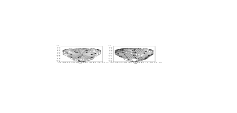
We depict in Fig. 7 the isoconditioning loci of matrix B. We notice that the loci of both working modes are identical. This is due to both the absence of joint limits on the actuated joints and the symmetry of the manipulator. For one configuration, only the signs of $m_{i}$ change from a working mode to another, but the condition number $\kappa$ is computed from the absolute values of $m_{i}$.

Figure 7: Isoconditioning loci of the matrix (a) ${\bf{B}}_{1}$ and (b) ${\bf{B}}_{2}$ with $R/r=2$ and $l/r=2$

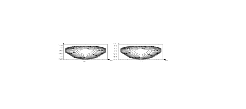
The shapes of the isoconditioning loci of $\overline{{\bf{K}}}$ (Fig. 8) are similar to those of the isconditioning loci of $\overline{{\bf{A}}}$; only the numerical values change.

Figure 8: Isoconditioning loci of the matrix (a) $\overline{{\bf{K}}}_{1}$ and (b) $\overline{{\bf{K}}}_{2}$ with $R/r=2$ and $l/r=2$

For the first working mode, the condition number of both matrices $\overline{{\bf{A}}}$ and $\overline{{\bf{K}}}$ decreases regularly around the isotropic configuration. The isoconditioning loci resemble concentric circles. However, for the second working mode, the isoconditioning loci of both matrices $\overline{{\bf{A}}}$ and $\overline{{\bf{K}}}$ resemble ellipses.

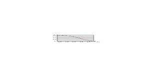
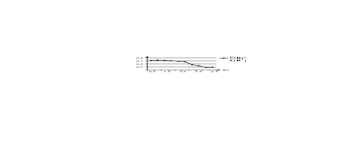
The characteristic length $L$ depends on $r$. Two indices can be studied according to parameter $R$: (i) the area of the Cartesian workspace, called $\cal S$, and (ii) the average of the conditioning, called $\overline{\kappa}$.

The first index is identical for the two working modes. Figure 9 depicts the variation of $S$ as a function of $R/r$, for $l/r=2$. Its maximum value is reached when $R/r=0.5$.

Figure 9: Variation of $\cal S$ as a function of $R/r$, with $l/r=2$

For the three matrices studied, $\overline{\kappa}$ can be regarded as a global performance index. This index thus allows us to compare the working modes. Figsures 10, 11 and 12 depict $\overline{\kappa}(\overline{{\bf{A}}})$, $\overline{\kappa}({\bf{B}})$ and $\overline{\kappa}(\overline{{\bf{K}}})$, respectively, as a function of $R/r$, with $l/r=2$.

Figure 10: $\overline{\kappa}(\overline{{\bf{A}}}_{1})$ and $\overline{\kappa}(\overline{{\bf{A}}}_{2})$ as a function of $R/r$, with $l/r=2$

Figure 11: $\overline{\kappa}({\bf{B}}_{1})$ and $\overline{\kappa}({\bf{B}}_{2})$ as a function of $R/r$, with $l/r=2$

Figure 12: $\overline{\kappa}(\overline{{\bf{K}}}_{1})$ and $\overline{\kappa}(\overline{{\bf{K}}}_{2})$ as a function of $R/r$, with $l/r=2$

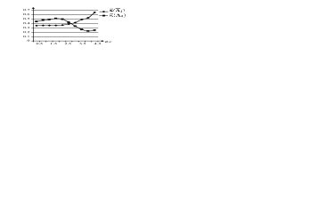
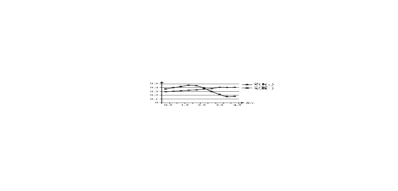
The value of $\overline{\kappa}(\overline{{\bf{A}}}_{1})$ increases with $R$. At the opposite, the maximum value of $\overline{\kappa}(\overline{{\bf{A}}}_{2})$ is reached when $R/r=2$. For both the working modes studied, $\overline{\kappa}({\bf{B}}_{1})$ and $\overline{\kappa}({\bf{B}}_{2})$ are identical for $R/r$ fixed. For the first working mode, the minimum value of $\overline{\kappa}(\overline{{\bf{K}}}_{1})$ and the maximum area of Cartesian workspace $\cal S$ occur at different values of $R/r$. This means that we must reach a compromise under these two indices. For the second working mode, there is an optimum of $\overline{\kappa}(\overline{{\bf{K}}}_{2})$ close to the optimum of $\cal S$, for $R/r=2$.

4 Conclusions

We produced the isoconditioning loci of the Jacobian matrices of a three-PRR parallel manipulator. This concept being general, it can be applied to any three-dof planar parallel manipulator. To solve the problem of nonhomogeneity of the Jacobian matrix, we used the notion of characteristic length. This length was defined for the isotropic configuration of the manipulator. The isoconditioning curves thus obtained characterize, for every posture of the manipulator, the optimum conditioning for all possible orientations of the end-effector. This index is compared with the area of Cartesian workspace and the conditioning average. The two optima being different, it is necessary to find another index to determine the optimum values. The results of this paper can be used to choose the working mode which is best suited to the task at hand or as a global performance index when we study the optimum design of this kind of manipulators.

References

- [1] [1] Lee, J., Duffy, J. and Hunt, K., A Pratical Quality Index Based on the Octahedral Manipulator, The International Journal of Robotic Research, Vol. 17, No. 10, October, 1998, 1081-1090.
- [2] [2] Angeles, J., Fundamentals of Robotic Mechanical Systems, Springer-Verlag, New York, 1997.
- [3] [3] Golub, G. H. and Van Loan, C. F., Matrix Computations, The John Hopkins University Press, Baltimore, 1989.
- [4] [4] Salisbury, J. K. and Craig, J. J., Articulated Hands: Force Control and Kinematic Issues, The International Journal of Robotics Research, 1982, Vol. 1, No. 1, pp. 4-17.
- [5] [5] Angeles, J. and López-Cajún, C. S. , Kinematic Isotropy and the Conditioning Index of Serial Manipulators, The International Journal of Robotics Research, 1992, Vol. 11, No. 6, pp. 560-571.
- [6] [6] Merlet, J. P., Les robots parallèles, 2nd édition, HERMES, Paris, 1997.
- [7] [7] Gosselin, C., Sefrioui, J., Richard, M. J., Solutions polynomiales au problème de la cinématique des manipulateurs parallèles plans à trois degré de liberté, Mechanism and Machine Theory, Vol. 27, pp. 107-119, 1992.
- [8] [8] Chablat, D. and Wenger, Ph., Working Modes and Aspects in Fully-Parallel Manipulator, Proceedings IEEE International Conference on Robotics and Automation, 1998, pp. 1964-1969.
- [9] [9] Gosselin, C. and Angeles, J., Singularity Analysis of Closed-Loop Kinematic Chains, IEEE, Transaction on Robotics and Automation, Vol. 6, pp. 281-290, June 1990.
- [10] [10] Ranjbaran, F., Angeles, J., González-Palacios, M. A. and Patel, R. V., The Mechanical Design of a Seven-Axes Manipulator with Kinematic Isotropy, Journal of Intelligent and Robotic Systems, 1995, Vol. 14, pp. 21-41.