Solute trapping and diffusionless solidification in a binary system

Abstract

Numerous experimental data on the rapid solidification of binary systems exhibit the formation of metastable solid phases with the initial (nominal) chemical composition. This fact is explained by complete solute trapping leading to diffusionless (chemically partitionless) solidification at a finite growth velocity of crystals. Special attention is paid to developing a model of rapid solidification which describes a transition from chemically partitioned to diffusionless growth of crystals. Analytical treatments lead to the condition for complete solute trapping which directly follows from the analysis of the solute diffusion around the solid-liquid interface and atomic attachment and detachment at the interface. The resulting equations for the flux balance at the interface take into account two kinetic parameters: diffusion speed $V_{DI}$ on the interface and diffusion speed $V_{D}$ in bulk phases. The model describes experimental data on nonequilibrium solute partitioning in solidification of Si-As alloys [M.J. Aziz et al., J. Cryst. Growth 148, 172 (1995); Acta Mater. 48, 4797 (2000)] for the whole range of solidification velocity investigated.

PACS numbers: 81.10.Aj; 05.70.Fh; 05.70.Ln; 81.30.Fb

I Introduction

The concept of “solute trapping” has been introduced to define the processes of solute redistribution at the interface which are accompanied by $(i)$ the increasing of the chemical potential bk1 and $(ii)$ the deviation of the partition coefficient for solute distribution towards unity from its equilibrium value (independently of the sign of the chemical potential) aziz4 .

In experimental investigations of rapid solidification, a complete solute trapping leading to diffusionless (chemically partitionless) solidification was first observed by Olsen and Hultgren and Duwez et al. in experiments on rapid solidification oh91 . They showed that rapidly solidifying alloy systems lead to the originating of supersaturated solid solution with the initial (nominal) chemical composition of the alloy. Later on, crystal microstructures with the initial chemical composition were found by Biloni and Chalmers in rapidly solidified pre-dendritic and dendritic patterns bicha .

Backer and Cahn bk1 have shown that with the finite solidification velocity in a Cd-Zn system the coefficient of the Cd distribution becomes equal to the unit that characterizes diffusionless solidification. This fact has been confirmed in many binary systems by Miroshnichenko mir . He investigated dendritic crystal microstructure after quenching from the liquid state by splat quenching and melt spinning methods. The results of Miroshnichenko’s microstructural analysis show that at a cooling rate greater than some critical value (depending on an alloy and experimental method this value is in the range $10^{5}-10^{6}$ K/s) a core of main stems of dendrites has initial (nominal) chemical composition of the alloy. A critical value for undercooling in the transition to purely thermally controlled growth with a homogeneous distribution of chemical composition in Ni-B solidifying samples processed by an electromagnetic levitation facility has been obtained by Eckler et al. eck . Finally, it is necessary to note that many eutectic systems undergo chemically partitionless solidification with an initial composition mir that can be explained by the transition to diffusionless solidification gh .

As a consequence, experimental investigations bk1 ; oh91 ; bicha ; mir ; eck show that with increasing driving force of solidification solute traps are much more pronounced by solidifying microstructure. At a finite value of the critical governing parameters (undercooling, cooling rate or temperature gradient) complete solute trapping occurs. Because the finite value of the governing parameter defines the concrete solidification velocity, complete solute trapping and diffusionless solidification begin to proceed with a fixed critical growth velocity of crystals.

The main purpose of the present paper is to describe a model for solute trapping and the transition from chemically partitioned to diffusionless solidification in a binary system. Using the local nonequilibrium approach to rapid solidification, an analysis of diffusion mass transport in bulk phases together with conditions of atomic attachment and detachment on the solid-liquid interface is given.

The paper is organized as follows. In Sec. II, previous investigations of solute trapping are shortly reviewed. In Sec. III, an analysis of solute diffusion leading to pronounced solute trapping and complete solute trapping is given. The nonequilibrium solute partitioning function for atoms on the interface is derived in Sec. IV. A comparison with previous models and experimental data on solidification of binary systems is presented in Sec. V. Finally, in Sec. VI conclusions of the work are summarized.

II Previous investigations

For the simplest case of an atomic system, let us consider an isobaric and isothermal binary system (the pressure $P$ and temperature $T$ are constant) with concentration $X_{A}$ and $X_{B}$ of atoms $A$ and $B$, respectively. In this article, we denote $X$ as the concentration of the atoms of $B$ sort. For a brief overview, we summarize the equilibrium and nonequilibrium solute distribution on the solid-liquid interface.

II.1 Equilibrium

In equilibrium, the concentration of atoms $X$ at the phase interface is not equal from both sides of the interface due to the different solubility of atoms in phases. During the equilibrium coexistence of phases (gas-solid, liquid-solid, gas-liquid) the atoms are distributed along the interface in consistency with the diagram of a phase state. A difference in atomic concentration in phases at the interface can be characterized by the equilibrium coefficient $k_{e}$ of the atomic distribution between phases. For equilibrium coexistence of phases (e.g., between crystal and melt, vapor and crystal, crystal and liquid), the coefficient $k_{e}$ can be expressed in the general form chernov1

$$k_{e}(X_{L},X_{S},T)=\frac{X_{S}^{e}}{X_{L}^{e}}\equiv\exp\left(-\frac{\Delta\mu^{\prime}}{RT}\right).$$ (1)

In Eq. (1), $X_{L}^{e}$ and $X_{S}^{e}$ are the mole fractions of the $B$ component in the liquid phase ($L$) or crystal ($S$), respectively, $R$ is the gas constant, and $\Delta\mu^{\prime}$ is the difference in chemical potentials described by

$$\Delta\mu^{\prime}=\Delta\mu_{B}^{\prime}-\Delta\mu_{A}^{\prime},$$ (2)

with

$$\Delta\mu_{B}^{\prime}=\mu_{BS}^{\prime}-\mu_{BL}^{\prime},\qquad\Delta\mu_{A}^{\prime}=\mu_{AS}^{\prime}-\mu_{AL}^{\prime},$$ (3)

where $\Delta\mu_{A}^{\prime}$ and $\Delta\mu_{B}^{\prime}$ are the driving forces for redistribution of atoms $A$ and $B$, respectively, which are defined by redistribution potentials $\mu_{A}^{\prime}$ and $\mu_{B}^{\prime}$ for phases $L$ and $S$. The differences $\Delta\mu_{A}^{\prime}$ and $\Delta\mu_{B}^{\prime}$, Eq. (3), define the sign of $\Delta\mu^{\prime}$ in Eq. (2). For instance, if $\Delta\mu^{\prime}$ is negative ($\Delta\mu_{A}^{\prime}>\Delta\mu_{B}^{\prime}$), one has $k_{e}<1$ - the case of smaller solubility of atoms $B$ in the phase $S$ in comparison with their solubility in the phase $L$.

As a general characteristic of phase equilibria in binary systems, expression (1), together with Eqs. (2) and (3), is usually considered as a measure of the driving force for atomic redistribution at the phase interface. It can also be considered as one of the main parameters for the construction of the diagrams of a phase state.

II.2 Nonequilibrium

Expressions (1)-(3) assume local equilibrium at the interface, which is a useful approximation for many systems transforming at small interface velocities. At a large driving force for the interface advancing and with increasing of the interface velocity, the local equilibrium is not maintained bk1 . Therefore, the condition for local interfacial equilibrium was relaxed by taking into account a kinetic interface undercooling and deviations from chemical equilibrium at the alloy’s solidification front chernov1 ; chernov .

A number of models hall ; chernov ; aziz4 ; chernov2 ; brice ; aziz3 have been proposed to account for solute trapping and related phenomena observed during rapid phase transformations. One of the well-established boundary conditions for solute redistribution can be taken from the continuous growth model (CGM) applied to solute trapping by Aziz and Kaplan aziz4 ; aziz3 ; aziz5 . The CGM assumes alloy solidification at a “rough interface”; i.e, all interface sites are potential sites for crystallization events. With a high solidification rate, the atom can be trapped on a high-energy site of the crystal lattice. This leads to a local nonequilibrium on the interface and to the formation of metastable solids (see examples in Ref. hghm ). As a result, the solute partitioning function at the solid-liquid interface is described by aziz3 ; aziz4

$$k(V)=\frac{k_{e}+V/V_{DI}}{1+V/V_{DI}},$$ (4)

where $V_{DI}$ is the speed of diffusion at the interface and $k_{e}$ is the value of the equilibrium partition coefficient given by Eq. (1), i.e., with the negligible interface motion, $V\rightarrow 0$. Equation (4) evaluates the ratio $X_{S}/X_{L}$ at the interface for dilute solutions of B (“solute”) in A (“solvent”).

The interfacial diffusion speed $V_{DI}$ is the kinetic parameter describing the deviation from chemical equilibrium at the interface. It has been defined as the ratio between the diffusion coefficient $D_{I}$ at the interface and the characteristic distance $\lambda$ for the diffusion jump aziz4 ; aziz3 : $V_{DI}=D_{I}/\lambda$. The distance $\lambda$ is assumed to be equal to the width of the solid-liquid interface (few interatomic distances) and the diffusion jumps are taken along the direction of growth. Therefore, this definition for $V_{DI}$ is corrected by results of molecular dynamic simulations cook . They include diffusion in all spatial directions; i.e., the diffusion speed is $V_{DI}=6D_{I}/\lambda$, where the factor of 6 accounts for the possibility of jumps along the six ($\pm x,y,z$) Cartesian axes.

Outcomes following from the solute partitioning function (4) were compared in the modeling of solute trapping using numerical computations based on the phase-field theory of alloys solidification. Wheeler et al. wbm2 naturally included an energy penalty for high composition gradients in the liquid that supresses the partitioning of solute at a rapidly moving interface and leads to solute trapping. They also showed that the construction of common tangents to the curves of free energy (in the spirit of Baker and Cahn bk2 ) has to be defined for nonequilibrium concentrations which already depend on the solidification velocity. In order to eliminate or reduce the solute trapping effect by the diffuse interface at small growth velocity, Karma and co-workers proposed an ad hoc suitable antitrapping condition to the diffusion flux karma_sol . These works wbm2 ; karma_sol showed that when the solute trapping effect comes to modeling alloy solidification with both phase and concentration fields, a crucial issue arises concerning the relative magnitudes of the gradients of the two fields within the solidification front as well as the relative thickness of the concentration jump interface. Additionally, Conti conti investigated the usual one-dimensional (1D) formulation of the phase field model without the concentration gradient corrections of Wheeler et al. wbm2 . He resolved the governing equations numerically for the interface temperature and the solute concentration field as a function of the growth velocity. The partition coefficient $k(V)$ is monotonically increasing towards unity at large growth rates following the predictions of the continuous growth model (4). However, in contrast to the results of natural experiments bk1 ; oh91 ; bicha ; mir ; eck , numeric predictions wbm2 ; conti were not able to reach the complete chemically partitionless (diffusionless) solidification at a finite solidification velocity.

One of the deficiencies of the function (4) is the difficulty to describe complete solute trapping at the finite solidification velocity: Equation (4) predicts $k\rightarrow 1$ only with $V\rightarrow\infty$. Contrary to this prediction, a transition to partitionless solidification occurs at a finite solidification velocity as it has been shown in numerous experiments oh91 ; bicha ; bk1 ; mir ; eck . Molecular dynamic simulations also show that the transition to complete solute trapping is observed at a finite interface velocity in rapid solidification of a binary system cook . Therefore, as an extension of Eq. (4), a generalized function for solute partitioning in the case of local nonequilibrium solute diffusion within the approximation of a dilute system has been introduced by Sobolev S1 . This yields

$$k(V)=\frac{(1-V^{2}/V_{D}^{2})k_{e}+V/V_{DI}}{1-V^{2}/V_{D}^{2}+V/V_{DI}},\qquad V<V_{D},$$

$$k(V)=1,\qquad V\geq V_{D}.$$ (5)

The diffusion speed $V_{D}$ introduced in Eq. (5) is the characteristic bulk speed. It is defined as a maximum speed for the solute diffusion propagation or as a speed for the front of solute diffusion profile. In particular, the speed $V_{D}$ is obtained by the speed of propagation of the plane harmonic wave away from the solid-liquid interface (see the Appendix in Ref. G2 ). As the velocity $V$ of the interface is comparable by magnitude to the speed $V_{D}$, the high frequency limit takes place: $\omega\tau_{D}>>1$, where $\omega$ is the real cyclic frequency of the plane harmonic wave and $\tau_{D}$ is the time for relaxation of the diffusion flux to its steady state. In this case, $V_{D}$ has to be considered finite and it is defined as $V_{D}=(D/\tau_{D})^{1/2}$, where $D$ is the diffusion coefficient in bulk liquid.

In the local equilibrium limit, i.e., when the bulk diffusive speed is infinite, $V_{D}\rightarrow\infty$, expression (5) reduces to the function $k(V)$ which takes into account the deviation from local equilibrium at the interface only as described by Eq. (4). The function (5) includes the deviation from local equilibrium at the interface (introducing interfacial diffusion speed $V_{DI}$) and in the bulk liquid (introducing diffusive speed $V_{D}$ in the bulk liquid). As Eq. (5) shows, complete solute trapping $k(V)=1$ proceeds at $V=V_{D}$. This result has been introduced by Sobolev from a postulation about the zero value for the diffusion coefficient at $V\geq V_{D}$. The next section further details that the condition for complete solute trapping follows directly from the analysis of solute diffusion flux.

III Diffusion mass transport and solute trapping

In 1D solidification along the $z$-axis, the mass balance is given by

$$\frac{\partial X}{\partial t}=-\frac{\partial J}{\partial z},$$ (6)

where $t$ is the time and $J$ is the diffusion flux. To consider solute trapping in 1D local nonequilibrium solidification, we take one of the results from a model of rapid phase transitions gj . Using this model, the evolution equation for diffusion flux $J$ along the z-axis is described by

$$J=M\left[\frac{\partial}{\partial z}\left(\frac{\partial s}{\partial X}+\varepsilon_{x}^{2}\frac{\partial^{2}X}{\partial z^{2}}\right)-\alpha_{j}\frac{\partial J}{\partial t}\right],$$ (7)

where $s$ is the entropy density, $\varepsilon_{x}$ the factor proportional to the correlation length, and $M$ is the diffusion mobility of atoms. The latter is defined by

$$M=T\overline{D},\qquad\overline{D}=D(\partial(\Delta\mu)/\partial X)^{-1},$$ (8)

where $D$ is the diffusion coefficient and $\Delta\mu$ is the difference of chemical potentials between solvent and solute. From known thermodynamic expressions j one can accept that

$$\frac{\partial s}{\partial X}=-\frac{\Delta\mu}{T},\qquad\alpha_{j}=\frac{\tau_{D}}{TD}\frac{\partial(\Delta\mu)}{\partial X}=\frac{\tau_{D}}{T\overline{D}},$$ (9)

where $\tau_{D}$ is the time for diffusion flux relaxation to its steady state. Then, omitting the term responsible for atomic correlation, i.e., assuming that $\varepsilon_{x}=0$, one can get from Eq. (7) the expression

$$J=M\left[\frac{1}{T}\frac{\partial(\Delta\mu)}{\partial z}-\frac{\tau_{D}}{T\overline{D}}\frac{\partial J}{\partial t}\right].$$ (10)

Using Eq. (8), the evolution equation (10) results as follows

$$\qquad J=-\overline{D}\frac{\partial(\Delta\mu)}{\partial z}-\tau_{D}\frac{\partial J}{\partial t}.$$ (11)

We find the solution for the diffusion flux $J$ which has significance in the analysis of solute trapping. Using the expression for the diffusion speed, $V_{D}=(D/\tau_{D})^{1/2}$, from Eqs. (6) and (11) one gets

$$\tau_{D}\frac{\partial^{2}J}{\partial t^{2}}+\frac{\partial J}{\partial t}=D\frac{\partial^{2}J}{\partial z^{2}}.$$ (12)

Equation (12) is a partial differential equation of hyperbolic type. It describes the flux $J$ in the so-called “hyperbolic evolution”, which proceeds with a sharp front of the profile for the solute transport. It occurs due to both the diffusive and propagative nature of the transport in the high frequency limit $\omega\tau_{D}>>1$ with $V\sim V_{D}$.

For a steady-state regime of interfacial motion Eq. (12) takes the form

$$D\left(1-\frac{V^{2}}{V_{D}^{2}}\right)\frac{d^{2}J}{dz^{2}}+V\frac{dJ}{dz}=0,$$ (13)

which is true in a reference frame moving at constant velocity $V$ with the interface $z=0$. A general solution of Eq. (13) is

$$J(z)=c_{1}+c_{2}\exp\left(-\frac{Vz}{D(1-V^{2}/V_{D}^{2})}\right).$$ (14)

To define a particular solution one can assume the following boundary conditions: the balance on the interface is $J(z=0)=V(X_{L}^{*}-X_{S}^{*})$, and the flux is limited by the expression $J(z\rightarrow\infty)=0$ far from the interface with $z\rightarrow\infty$. The latter condition gives $c_{1}=0$ for any velocity $V$ and one gets $c_{2}=0$ for $V\geq V_{D}$. Also, from the interfacial balance with $z=0$ one gets $c_{2}=V(X_{L}^{*}-X_{S}^{*})$ for $V<V_{D}$. As a result, solution (14) transforms into the particular solution

$$J(z)$$

$$=V(X_{L}^{*}-X_{S}^{*})\exp\left(-\frac{Vz}{D(1-V^{2}/V_{D}^{2})}\right),\qquad V<V_{D},$$

$$J(z)=0,\qquad V\geq V_{D},$$ (15)

where $X_{L}^{*}$ and $X_{S}^{*}$ are the liquid concentration and solid concentration, respectively, on the interface.

Solution (15) gives the condition for complete solute trapping with finite velocity $V\geq V_{D}$. This is expressed by the expression for the solute partitioning function

$$k(V)=X_{S}^{*}/X_{L}^{*}\neq 1,\qquad V<V_{D},$$

$$k(V)=1,\qquad X_{S}^{*}=X_{L}^{*},\qquad V\geq V_{D}.$$ (16)

The latter condition in Eq. (16) defines the equality of the concentrations in the phases and leads to complete solute trapping.

To obtain an explicit form for the solute partitioning function (16), we analyze the balance of diffusion fluxes on the interface. Taking again the steady state regime of solidification constant velocity $V$, from the system (6) and (11) one can obtain the equations

$$\frac{dJ}{dz}=V\frac{dX}{dz},\qquad J=-\overline{D}\frac{d(\Delta\mu)}{dz}+\tau_{D}V\frac{dJ}{dz},$$ (17)

from which we get the single equation for the diffusion flux $J$. This yields

$$J=-D\left(\frac{\partial(\Delta\mu)}{\partial X}\right)^{-1}\frac{d(\Delta\mu)}{dz}+D\frac{V^{2}}{V_{D}^{2}}\frac{dX}{dz}.$$ (18)

The above-defined thermodynamic parameter $\overline{D}$ and the diffusion speed $V_{D}$ in bulk have been taken into account. Defining the gradient of the difference of the chemical potentials as $d(\Delta\mu)/dz=[\partial(\Delta\mu)/\partial X]dX/dz$, Eq. (18) gives

$$J=-D\left(\frac{\partial(\Delta\mu)}{\partial X}\right)^{-1}\left[1-\frac{V^{2}}{V_{D}^{2}}\right]\frac{d(\Delta\mu)}{dz}.$$ (19)

This equation is a general expression for the steady diffusion flux into the liquid from the interface. Within the local equilibrium limit $V_{D}\rightarrow\infty$ one can obtain the known Fickian approximation which has been used previously for analysis of solute trapping Kurz-Fisher ; ahmad .

Analytical solutions GS for solidification under local nonequilibrium diffusion show that the concentration in both phases becomes equal to the initial (nominal) concentration and the diffusion flux is absent for $V\geq V_{D}$. It is also given by Eq. (15). Therefore, in addition to Eq. (19), one can finally obtain

$$J=-D\left(\frac{\partial(\Delta\mu)}{\partial X}\right)^{-1}\left[1-\frac{V^{2}}{V_{D}^{2}}\right]\frac{d(\Delta\mu)}{dz},\qquad V<V_{D},$$

$$J=0,\qquad V\geq V_{D}.$$ (20)

At the phase interface one assumes in Eq. (20), first, that the term $D((\partial\Delta\mu)/\partial X)^{-1}$ is proportional to concentration such that

$$D\left(\frac{\partial(\Delta\mu)}{\partial X}\right)^{-1}=\frac{D_{I}X_{L}^{*}}{RT}.$$ (21)

Second, the chemical inhomogeneity (solutal segregation) exists due to the jump of the chemical potential $\Delta\mu$ which has the interfacial gradient $-d(\Delta\mu)/dz\cong\Delta\mu/W_{0}$ at a small distance $W_{0}$ of the order of a few interatomic distances. Third, in an approximation of ideal (or even real) solutions, one can assume for the interfacial difference of chemical potentials $\Delta\mu=\Delta\mu^{L}(X)-\Delta\mu^{S}(X)\cong RT(\ln X_{L}^{e}-\ln X_{L}^{*})-RT(\ln X_{S}^{e}-\ln X_{S}^{*})=RT\ln(X_{S}^{*}/X_{L}^{*})-RT\ln(X_{S}^{e}/X_{L}^{e})=RT[\ln k(V)-\ln k_{e}]$, where $X_{L}^{e}$ and $X_{S}^{e}$ are equilibrium concentrations on the interface from the liquid phase and solid phase, respectively, and $k(V)$ is the ratio of concentrations on the interface defined by Eq. (16). Taking into account these last evaluations, one can get for the chemical potential gradient the expression

$$-\frac{d(\Delta\mu)}{dz}\cong\frac{RT}{W_{0}}\ln\frac{k(V)}{k_{e}}.$$ (22)

Integration of the balance (17) on the interface gives the flux

$$J=V(X_{L}^{*}-X_{S}^{*}).$$ (23)

Substituting Eqs. (21) and (22) into the expression for diffusion flux Eq. (20) with using the balance (23) gives the following expression for the solute partitioning function:

$$\left[1-\frac{V^{2}}{V_{D}^{2}}\right]\ln\frac{k(V)}{k_{e}}=\frac{V}{V_{DI}}[1-k(V)],\qquad V<V_{D},$$

$$k(V)\equiv X_{S}^{*}/X_{L}^{*}=1,\qquad V\geq V_{D},$$ (24)

where $V_{DI}=D_{I}/W_{0}$ is the speed for solute diffusion on the interface.

Equation (24) gives the evaluation of solute trapping effect through the solute partitioning function $k(V)$ derived initially from the analysis of the evolution equation (7) for the diffusion flux $J$. This equation takes into account finite diffusion speeds on the interface and in bulk liquid. The introduction of these two speeds is a consequence of the local nonequilibrium both on the interface and in bulk liquid. As Eq. (24) shows, the complete solute trapping $k(V)=1$ proceeds at $V=V_{D}$. Equation (24) transforms into a previously known expression for the function $k(V)$ derived in Refs. Kurz-Fisher ; ahmad with relaxing local equilibrium on the interface and using local equilibrium in bulk liquid ($V_{D}\rightarrow\infty$) for the diluted binary system ($X_{L}^{*}<<1$).

IV Solute partitioning function

We use a model of diffusion in which particles move by diffusion jumps in random time between two phases (states). This model was called the “two-level model of diffusion” and it was introduced in the context of various application, e.g., in chromatography ge or for a longitudinal solute dispersion in a tube with flowing water (Taylor’s dispersion) tay1 .

Let $P_{i}(t,z)$ be the probability density of a particle position in the phase $i=L$ or in the phase $i=S$ at the moment $t$. Then local conservation of the probability density in a point with coordinate $z$ belonging to the phase $i$ is defined by

$$\frac{\partial P_{i}}{\partial t}=-\frac{\partial J_{i}}{\partial z}.$$ (25)

If the interface moves with a velocity comparable to the solute diffusion speed $V_{D}$ in bulk phases, then the flux $J_{i}(t,z)$ of the density probability depends on the prehistory of the diffusion process. The flux, therefore, is defined by

$$J_{i}(t,z)=-\int^{t}_{-\infty}D_{i}(t-t^{*})\frac{\partial P_{i}(t^{*},z)}{\partial z}dt^{*}.$$ (26)

The relaxation function $D_{i}(t-t^{*})$ can be chosen in the form $D_{i}(t-t^{*})=D_{i}(0)\exp[-(t-t^{*})/\tau_{D}]$ of exponential decay. In such a case, Eq. (26) is reduced to the Maxwell-Kattaneo equation

$$\tau_{D}\frac{\partial J_{i}}{\partial t}+J_{i}+D_{i}(0)\frac{\partial P_{i}}{\partial z}=0.$$ (27)

It is accepted in Eq. (27) that $D_{i}(0)$ is the diffusion coefficient at the final moment of relaxation prehistory so that $D_{i}(0)=D$. System (25) and (27) gives a single equation of a hyperbolic type for the density of probability

$$\tau_{D}\frac{\partial^{2}P_{i}}{\partial t^{2}}+\frac{\partial P_{i}}{\partial t}=D_{i}\frac{\partial^{2}P_{i}}{\partial z^{2}},$$ (28)

or for the flux,

$$\tau_{D}\frac{\partial^{2}J_{i}}{\partial t^{2}}+\frac{\partial J_{i}}{\partial t}=D_{i}\frac{\partial^{2}J_{i}}{\partial z^{2}}.$$ (29)

As was shown in Ref. cz , the density of probability described by Eq. (28) gives a positive entropy production for the particle exchange between two levels (between two subsystems or phases).

Integration of Eq. (28) by an infinitesimal layer including an interface leads to the balance

$$\left[D_{i}\frac{\partial P_{i}}{\partial z}+\tau_{D}\frac{\partial(VP_{i})}{\partial t}+J_{i}\right]\bigg{|}^{L}_{S}=0.$$ (30)

In the steady-state regime one can get the following equation for the i-th phase

$$D_{i}\frac{\partial P_{i}}{\partial z}+\tau_{D}\frac{\partial(VP_{i})}{\partial t}+J_{i}=D_{i}\frac{dP_{i}}{dz}-\tau_{D}V^{2}\frac{dP_{i}}{dz}+J_{i}$$

$$=D_{i}\left(1-\frac{V^{2}}{V_{Di}^{2}}\right)\frac{dP_{i}}{dz}+J_{i},$$ (31)

which is true in a reference frame moving with constant velocity $V$ and placed on the interface where the balance (25) is described as $dJ_{i}/dz=VdP_{i}/dz$. Using Eq. (31), the balance (30) is

$$J_{L}-J_{S}$$

$$=-\left[D_{L}\left(1-\frac{V^{2}}{V_{DL}^{2}}\right)\frac{dP_{L}}{dz}-D_{S}\left(1-\frac{V^{2}}{V_{DS}^{2}}\right)\frac{dP_{S}}{dz}\right].$$

(32)

In Eq. (32) we introduce the speeds $V_{DL}$ and $V_{DS}$ of interfacial solute diffusion from the liquid and solid phases, respectively. They are defined by

$$V_{DL}=D_{L}/l_{D}=\nu_{L}l_{D},\qquad V_{DS}=D_{S}/l_{D}=\nu_{S}l_{D},$$ (33)

where $D_{L}$ and $D_{S}$ are the diffusion coefficients in the phases, $l_{D}$ scales for diffusion within which the diffusion jumps occur in phases (or on the interface), and $\nu_{L}$ and $\nu_{S}$ are the frequencies of diffusion jumps in phases (or on the interface). From the theory of the transitive state christ one can define the frequencies of atomic jumps as

$$\nu_{L}=\nu_{0}\exp\left(-\frac{Q_{D}}{RT}\right),$$

$$\nu_{S}=\nu_{0}\exp\left(-\frac{Q_{D}+\Delta\mu^{\prime}}{RT}\right),$$ (34)

where $\nu_{0}$ is the attempt frequency of atomic jumps of the order of the vibrational frequency chernov1 ; vin , $Q_{D}$ the activation barrier for atomic diffusion through the interface, and $\Delta\mu^{\prime}$ is the difference of chemical potentials defined by Eqs. (2) and (3). Obviously, interfacial equilibrium exists for

$$\nu_{S}/\nu_{L}=\exp[-\Delta\mu^{\prime}/(RT)]\equiv k_{e}.$$ (35)

From the interfacial balance (32) there follows

$$J_{L}-J_{S}=-\left(1-\frac{V^{2}}{V_{DL}^{2}}\right)\frac{d}{dz}\left[D_{L}P_{L}-D_{S}(V)P_{S}\right],$$ (36)

where $D_{S}(V)$ is the function of the interfacial velocity $V$ defined by

$$D_{S}(V)=D_{S}\frac{1-V^{2}/V_{DS}^{2}}{1-V^{2}/V_{DL}^{2}}$$

$$=\left\{\begin{array}[]{ll}0,&V_{DS}<<V_{DL},\\ \\ D_{S},&V_{DS}\approx V_{DL},\\ \\ D_{S}(1-V^{2}/V_{DL}^{2})^{-1},&V_{DS}\rightarrow\infty.\end{array}\right.$$ (42)

The function (42) describes the following cases: (a) $V_{DS}\rightarrow 0$, negligible diffusion in solid ($D_{S}=0$) in comparison with the diffusion in liquid; (b) $V_{DS}\approx V_{DL}$, approximate equality for diffusion speeds in the liquid and solid around the interface; and (c) $V_{DS}\rightarrow\infty$, condition of local equilibrium in the diffusion field of the solid (that occurs with high frequency jumps of atoms in solid).

From now on, the above case (b) for approximate equality of diffusion speeds in phases around the interface is taken. First, we use the finite difference $-dx=l_{D}$ in the balance (32). Second, we take into account that the factor $(1-V^{2}/V_{DL}^{2})$ is related to the bulk diffusion. Finally, using the definition (33), the balance (32) is described by

$$J_{L}-J_{S}=\left(1-\frac{V^{2}}{V_{D}^{2}}\right)[V_{DL}P_{L}-V_{DS}P_{S}],$$ (43)

where $V_{D}$ is the solute diffusion speed in bulk liquid around the interface. Using Eqs. (33)-(35), this balance can be rewritten as

$$J_{L}-J_{S}=V_{DL}\left(1-\frac{V^{2}}{V_{D}^{2}}\right)[P_{L}-k_{e}P_{S}].$$ (44)

For the concentrated binary system the probabilities $P_{L}$ and $P_{S}$ in Eq. (44) are directly proportional to the atomic concentrations in phases. This leads to

$$P_{L}=X_{S}(1-X_{L})/\Omega,\quad P_{S}=X_{L}(1-X_{S})/\Omega,$$ (45)

where $\Omega$ is the atomic volume. Therefore, Eq. (44) can be rewritten as

$$J_{L}-J_{S}=\left(1-\frac{V^{2}}{V_{D}^{2}}\right)$$

$$\times[X_{S}(1-X_{L})-k_{e}X_{L}(1-X_{S})]\frac{V_{DL}}{\Omega}.$$ (46)

We further use the already obtained result (20) according to which the diffusion flux is absent at $V\geq V_{D}$. Then, the difference (46) of fluxes on the interface takes the form

$$J_{L}-J_{S}=\left(1-\frac{V^{2}}{V_{D}^{2}}\right)$$

$$\times[X_{S}(1-X_{L})-k_{e}X_{L}(1-X_{S})]\frac{V_{DL}}{\Omega},\qquad V<V_{D},$$

$$J_{L}=J_{S},\qquad V\geq V_{D}.$$ (47)

The net flux (47) must be equal to the diffusion flux

$$J_{D}=(X_{L}-X_{S})\frac{V}{\Omega}.$$ (48)

From the equality of Eqs. (47) and (48) one gets

$$(X_{L}-X_{S})\frac{V}{V_{DI}}=\left(1-\frac{V^{2}}{V_{D}^{2}}\right)$$

$$\times[X_{S}(1-X_{L})-k_{e}X_{L}(1-X_{S})],\qquad V<V_{D},$$

$$X_{L}=X_{S},\qquad V\geq V_{D},$$ (49)

in which $V_{DI}=V_{DL}$ is the diffusion speed on the interface from the liquid phase. Equation (49) can be easily resolved regarding the function $k(V)=X_{S}/X_{L}$ of nonequilibrium solute partitioning. This yields

$$k(V,X_{L}^{*})$$

$$=\displaystyle\frac{(1-V^{2}/V_{D}^{2})k_{e}+V/V_{DI}}{(1-V^{2}/V_{D}^{2})[1-(1-k_{e})X_{L}^{*}]+V/V_{DI}},\quad V<V_{D},$$

$$k(V,X_{L}^{*}=X_{0})=1,\qquad V\geq V_{D},$$ (50)

where $X_{L}^{*}$ is the solute concentration in the liquid at the interface.

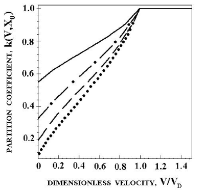
Figure 1: Predictions of the model given by Eq. (52). Constants of the binary system are equilibrium partition coefficient $k_{e}=0.1$, bulk diffusion speed $V_{D}=25$ (m/s), and interface diffusion speed $V_{DI}=20$ (m/s). The curves present: diluted system, $(1-k_{e})X_{0}<<1$ (dotted line); slightly concentrated system, $X_{0}=0.10$ (dashed line); concentrated system $X_{0}=0.25$, (dash-dotted line); and equiconcentrated system, $X_{0}=0.50$ (solid line).

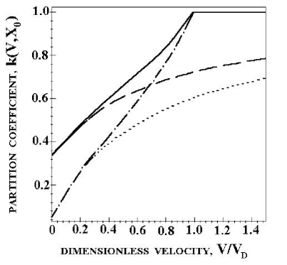
Figure 2: Nonequilibrium solute partitioning function $k(V,X_{0})$ given by the various models. Constants of the binary system are nominal concentration of a solute $X_{0}=0.05$ mole fraction, equilibrium partition coefficient $k_{e}=0.22$, bulk diffusion speed $V_{D}=19$ (m/s), and interface diffusion speed $V_{DI}=16$ (m/s). The dotted line is given by the model of Aziz aziz3 for the diluted system $(1-k_{e})X_{0}<<1$, the dashed line is given by the model of Aziz and Kaplan aziz4 , the dash-dotted line is given by the model of Sobolev S1 for diluted system, and the solid line is predicted by the present model given by Eq. (52).

V Discussion and comparison with experimental data

Expression (50) gives the general functional dependence of solute partitioning at the phase interface for concentrated binary systems, and with application to rapid solidification, it exhibits the two known limits. In the first limit, when solidification proceeds with local nonequilibrium at the interface only, i.e., with $V_{D}\rightarrow\infty$, Eq. (50) leads to the solute partitioning function of Aziz and Kaplan aziz4 . In the second limit, as the concentration $X_{L}^{*}$ of the second dissolved component becomes small, i.e., the term $(1-k_{e})X_{L}^{*}$ might be negligible in comparison with the unity, Eq. (50) transforms into Eq. (5) as suggested by Sobolev S1 .

From the analytical solution of the problem of rapid solidification under the steady-state regime GS , the concentration at the planar interface is given by

$$X_{L}^{*}=\frac{X_{0}}{k(V)},\qquad V<V_{D},$$

$$X_{L}^{*}=X_{0},\qquad V\geq V_{D},$$ (51)

where $X_{0}$ is the nominal (initial) concentration of the solute in the system. In accordance with the solutions obtained in Refs. GS , a source of concentration perturbations, i.e., the solid-liquid interface, moving at a velocity $V$ equal to or higher than the maximum speed $V_{D}$ of these perturbations, cannot change the concentration or create the concentration profile ahead of itself. As a result for the interface, one obtains in Eq. (51) that $X_{L}=X_{S}=X_{0}$ with $V\geq V_{D}$. Then the substitution of Eq. (51) into Eq. (50) leads to the following expression for nonequilibrium solute partitioning function:

$$k(V,X_{0})$$

$$=\frac{(1-V^{2}/V_{D}^{2})[k_{e}+(1-k_{e})X_{0}]+V/V_{DI}}{1-V^{2}/V_{D}^{2}+V/V_{DI}},V<V_{D},$$

$$k(V,X_{0})=1,\qquad V\geq V_{D}.$$ (52)

Figure 1 demonstrates the behavior of solute partitioning, Eq. (52), as a function of the interface velocity at various nominal solute concentrations. As the system deviates from a diluted one, the trapping of a solute becomes much more pronounced. Also, Eq. (52) shows that, independently from the solute concentration within the system, the complete solute trapping $k(V,X_{0})=1$ proceeds when the interface velocity becomes equal to or greater than the diffusion speed, i.e., with $V\geq V_{D}$. The condition of equality of concentrations in the liquid and solid [see Eqs. (49) and (50)] means that the lines of the nonequilibrium kinetic liquidus and solidus in the kinetic phase diagram are merging. It can also be considered as the characteristics of diffusionless processes.

As a general outcome, Eq. (52) includes the following important cases for nonequilibrium phase transformations: (i) the dilute limit described by Aziz’s model aziz3 , Eq. (4),

$$(1-k_{e})X_{0}<<1,~{}~{}and~{}V_{D}\rightarrow\infty,$$

(ii) the dilute limit described by Sobolev’s solute partitioning function, Eq. (5),

$$(1-k_{e})X_{0}<<1,~{}~{}and~{}with~{}the~{}finite~{}V_{D},$$

(iii) the concentrated system described by Aziz and Kaplan’s model, Ref. aziz4 ,

$$V_{D}\rightarrow\infty,~{}~{}for~{}arbitrary~{}concentration~{}X_{0}.$$

In comparison with the present model’s prediction described by Eq. (52) these limits are plotted in Fig. 2.

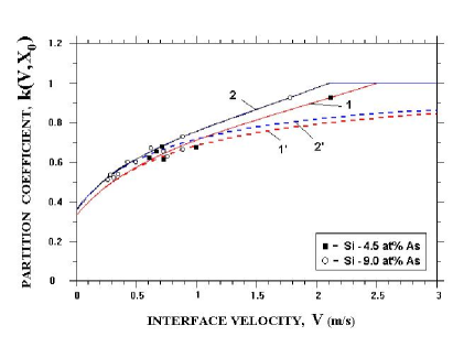
Figure 3: Solute partitioning versus interface velocity for experimental data aziz1 ; aziz2 on solidification of Si-As alloys. Curves $1^{\prime}$ and $2^{\prime}$ are given by Eq. (52) with $V_{D}\rightarrow\infty$ for 4.5 at.% and 9.0 at.% of As in Si, respectively (that gives the model of Azis and Kaplan aziz4 ). They describe experiment at small and moderate solidification velocities. Curves $1$ and $2$ are given by (52) with the finite speed $V_{D}$ for 4.5 at.% and 9.0 at.% of As in Si, respectively. These show ability to describe experiment in a whole region of investigated solidification velocities for both alloys. Data for calculations are given in Table 1.

Figure 3 exhibits theoretical predictions for solute partitioning in comparison with experimental data on the solidification of Si-As alloys. Introducing the deviation from equilibrium at both the interface and bulk liquid allows one to describe the whole set of experimental data. Particularly, the complete solute trapping is predicted by Eq. (52) for Si-4.5 at.%As with $V_{D}=2.5$ m/s and for Si-9.0 at.%As with $V_{D}=2.1$ m/s (Table 1). This provides a much better agreement with experiments than that shown by the Aziz-Kaplan model.

As can be seen in Fig. 3, predictions of the model of Azis and Kaplan [Eq. (52) with $V_{D}\rightarrow\infty$] disagree with experimental data in the region $1.7<V$ (m/s)$<2.2$ of solidification velocities. One may note that at the same solidification velocity, i.e., below about V = 2 (m/s), the ”interface temperature - velocity” relationship also exhibits a clear deviation from experimental data (see Fig. 11 in Ref. aziz2 ). One may also attribute this deviation to the increasing influence of local nonequilibrium solute diffusion around the interface and intensive solute trapping. Thermodynamic analysis and numeric evaluations confirm the idea about the pronounced influence of local equilibrium in bulk liquid on solute trapping and ”interface temperature - velocity” relationship at high solidification velocity G2 ; Gmater2 . This example confirms that local nonequilibrium in the solute diffusion field is responsible for nonequilibrium effects appearing in rapid solidification (such as solute trapping and solute drag) and essential influence on the interface response functions (temperature, concentration, velocity) Gmater2 . Thus, the agreement between Eq. (52) and experimental data demonstrates the pronounced effect of deviation from local equilibrium in bulk liquid on solute trapping at higher solidification velocity.

Table 1: Interface diffusion speed $V_{DI}$ and bulk diffusion speed $V_{D}$ for binary systems used in the calculations of the partitioning function $k(V,X_{0})$ at the solid-liquid planar interface. Equilibrium partition coefficient is taken as $k_{e}$=0.3 from Refs. aziz1 ; aziz2 .

Model	Binary system	$V_{DI}$ (m/s)	$V_{D}$ (m/s)	Reference
Aziz and Kaplan’s model, Ref. aziz4	Si - 4.5 at.% As	0.46	–	aziz1
		0.37	–	aziz2
Aziz and Kaplan’s model, Ref. aziz4	Si - 9 at.% As	0.46	–	aziz1
		0.37	–	aziz2
Sobolev’s solute partitioning function, Eq. (5)	Si - 4.5 at.% As	0.75	2.7	S1
	and Si - 9 at.% As
Present model, Eq. (52)	Si - 4.5 at.% As	0.8	2.5	current data
	Si - 9 at.% As	0.8	2.1	G2

Summarizing the behavior for solute partitioning shown in Figs. 1-3, one can conclude that during rapid solidification the consequences of deviations from local chemical equilibrium are threefold. First, the partition coefficient becomes dependent on the growth velocity. Second, the liquidus and solidus lines approach each other. For these two cases it can be enough to introduce into the theory deviation from local equilibrium at the interface only. Third, in the extreme case (if the solidification velocity is equal to or greater than the atomic diffusive speed in bulk liquid) the partition coefficient $k(V)$ becomes unity and the liquidus and solidus lines coincide. This leads to a solid being far from chemical equilibrium upon diffusionless solidification. Such three conditions are of special importance in the preparation of metastable supersaturated solutions hghm .

VI Conclusions

Solute trapping in rapid solidification of a binary alloy’s system has been considered. It has been shown that the condition for complete solute trapping leading to diffusionless solidification follows directly from the solution for the diffusion task. This task assumes both the low-frequency regime (purely diffusion) and high-frequency regime (diffusion and propagative regime) of atomic motion in a phenomenological statement.

The two-level model has been used to define the solute partitioning function. This model has been used previously (e.g., in chromatography and for investigation of longitudinal solute dispersion), and it has been formally reduced to expressions for an extended version of the continuous growth model. The extended version adopts two kinetic parameters: solute diffusion speed $V_{DI}$ on the interface and solute diffusion speed $V_{D}$ in bulk liquid.

A condition of complete solute trapping at the finite solidification velocity equal to the diffusion speed, $V=V_{D}$, has been found. This fact is expressed by the general expression (16) for the solute partitioning function. This condition defines the equality of the concentration in the phases and describes complete solute trapping. Analysis leads to concrete forms for the solute partitioning function. The first function is given by Eq. (24) and the second function for solute partitioning is described by Eq. (50). Both these functions predict a sharp finishing of solute trapping and the onset of diffusionless crystal growth at the solidification velocity $V$ equal to the solute diffusion speed $V_{D}$ in bulk liquid. A concrete expression for the liquid concentration $X_{L}^{*}$ at the interface allows us to give predictions comparable with experimental data.

The model predicts the complete behavior for the solute partitioning function dependent on the solidification velocity and alloy concentration. In comparison with the experimental data of Aziz et al. on solidification of Si-As alloys [M.J. Aziz et al., J. Cryst. Growth 148, 172 (1995); Acta Mater. 48, 4797 (2000)], the model well predicts deviation of the solute partitioning from equilibrium and complete solute trapping (Fig. 3). The transition from chemically partition growth to diffusionless growth at $V=V_{D}$ occurs sharply. As has been shown for dendritic growth GD1 such a sharp transition leads to an abrupt exchange of growth kinetics in consistency with experimental data.

- (1) J.C. Baker and J.W. Cahn, Acta Metall. 17, 575 (1969); in Solidification, edited by T.J. Hughel and G.F. Bolling (American Society of Metals, Metals Park, OH, 1971) p.23.
- (2) M.J. Aziz and T. Kaplan, Acta Metall. 36, 2335 (1988).
- (3) W.T. Olsen and R. Hultgren, Trans. AIME, 188 1323 (1950); P. Duwez, R.H. Willens, and W. Klement (Jr.) J. Appl. Phys. 31, 1136 (1960).
- (4) H. Biloni and B. Chalmers, Transactions AIME 233, 373 (1965).
- (5) I.S. Miroshnichenko, Quenching From the Liquid State (Metallurgia, Moscow, 1982).
- (6) K. Eckler, R.F. Cochrane, D.M. Herlach, B. Feuerbacher, and M. Jurisch, Phys. Rev. B 45, 5019 (1992).
- (7) P.K. Galenko and D.M. Herlach, Phys. Rev. Lett. 96, 150602 (2006).
- (8) A.A. Chernov, in Modern Crystallography, edited by M. Cardona, P. Fulde and H.-J. Queisser, Springer Series in Solid-State Science Vol.36 (Springer, Berlin, 1984), Vol.III, Chap.4.
- (9) R.N. Hall, J. Phys. Chem. 57, 836 (1953).
- (10) A.A. Chernov, Sov. Phys. Uspekhi 13, 101 (1970).
- (11) A.A. Chernov, in Rost Kristallov, edited by A.V. Shubnikov and N.N. Sheftal, Vol.3, (Akademia Nauk SSSR, Moscow, 1959) [English translation: ”Growth of Crystals”, vol.3 (Consultants Buro, New York, 1962) p.35]; V.V Voronkov and A.A. Chernov, Sov. Phys. Crystallogr. 12, 186 (1967).
- (12) J.C. Brice, The Growth of Crystals from the Melt (North-Holland, Amsterdam, 1965), p. 65; K.A. Jackson, G.H. Gilmer, and H.J. Leamy, in Laser and Electron Processing of Materials, edited by C.W. White and P.C. Peercy (Academic Press, New York, 1980), p. 104; R.F. Wood, Appl. Phys. Lett. 37, 302 (1980); D.E. Temkin, Sov. Phys. Crystallogr. 32(6), 782 (1988).
- (13) M.J. Aziz, J. Appl. Phys. 53, 1158 (1982).
- (14) M.J. Aziz and W.J. Boettinger, Acta Metall. Mater. 42, 527 (1994); M.J. Aziz, Metall. Mater. Trans 27A, 671 (1996).
- (15) D. Herlach, P. Galenko, and D. Holland-Moritz, Metastable Solids From Undercooled Melts (Elsevier, Amsterdam, 2007).
- (16) S.J. Cook and P. Clancy, J. Chem. Phys. 99, 2175 (1993).
- (17) A.A. Wheeler, W.J. Boettinger, and G.B. McFadden, Phys. Rev. E 47, 1893 (1993); W.J. Boettinger, A.A. Wheeler, B.T. Murray, and G.B. McFadden, Mater. Sci. Eng. A 178, 217 (1994).
- (18) J. C. Baker and J. W. Cahn, Solidification (ASM, Metals Park, OH, 1971), p. 23.
- (19) A. Karma, Phys. Rev. Lett. 87, 115701 (2001); J.J. Hoyt, M. Asta, and A. Karma, Mater. Sci. Eng. R 41(6), 121 (2003); J.C. Ramirez, C. Beckermann, A. Karma, and H.-J. Diepers, Phys. Rev. E 69, 051607 (2004); B. Echebarria, R. Folch, A. Karma, and M. Plapp, Phys. Rev. E 70, 061604 (2004).
- (20) M. Conti, Phys. Rev. E 56, 3717 (1997).
- (21) S.L. Sobolev, Phys. Status Solidi A 156, 293 (1996).
- (22) P. Galenko, Phys. Rev. B 65, 144103 (2002).
- (23) P. Galenko and D. Jou, Phys. Rev. E 71, 046125 (2005).
- (24) D. Jou, J. Casas-Vazquez, and G. Lebon, Extended Irreversible Thermodynamics, 2nd Edition (Springer, Berlin, 1996).
- (25) W. Kurz and D.J. Fisher, Fundamentals of Solidification, 3rd ed. (Trans Tech, Aedermannsdorf, 1992).
- (26) N.A. Ahmad, A.A. Wheeler, W.J. Boettinger, and G.B. McFadden, Phys. Rev. E 58, 3436 (1998).
- (27) P. Galenko and S. Sobolev, Phys. Rev. E 55, 343 (1997); P.K. Galenko and D.A. Danilov, J. Cryst. Growth 216, 512 (2000); Phys. Lett. A 272, 207 (2000); Phys. Rev. E 69, 051608 (2004).
- (28) J.C. Giddings and H. Eyring, J. Phys. Chem. 59, 416 (1955); J.C. Giddings, J. Chem. Phys. 26, 169 (1955).
- (29) G.I. Taylor, Proc. R. Soc. London, Ser. A 219, 186 (1953); ibidem 223, 446 (1954); Van Den C. Broeck, Physica A 186, 677 (1990).
- (30) J. Camacho and M. Zakari, Phys. Rev. E 50, 4233 (1994).
- (31) J.W. Christian, The Theory of Transformations in Metals and Alloys, 2nd Edition (Pergamon Press, Oxford, 1975), P. 1, Chapt. 3.
- (32) G.H. Vineyard, J. Phys. Chem. Solids 3, 121 (1957).
- (33) J.A. Kittl, M.J. Aziz, D.P. Brunco, and M.O. Thompson, J. Cryst. Growth 148, 172 (1995).
- (34) J.A. Kittl, P.G. Sanders, M.J. Aziz, D.P. Brunco, and M.O. Thompson, Acta Mater. 48, 4797 (2000).
- (35) P. Galenko, Mater. Sci. Eng. A 375-377, 493 (2004).
- (36) P.K. Galenko and D.A. Danilov, Phys. Lett. A 235, 271 (1997); J. Cryst. Growth 197, 992 (1999).