Superconductivity in zigzag CuO chains

Abstract

Superconductivity has recently been discovered in Pr₂Ba₄Cu₇O_15-δ with a maximum $T_{c}$ of about 15K. Since the CuO planes in this material are believed to be insulating, it has been proposed that the superconductivity occurs in the double (or zigzag) CuO chain layer. On phenomenological grounds we propose a theoretical interpretation of the experimental results in terms of a new phase for the zigzag chain, labelled by C₁S${}_{\frac{3}{2}}$. This phase has a gap in the relative charge mode and a partial gap in the relative spin mode. It has gapless uniform charge and spin excitations and can have a divergent superconducting susceptibility, even for repulsive interactions. A microscopic model for the zigzag CuO chain is proposed, and on the basis of density matrix renormalization group (DMRG) and bosonization studies, we adduce evidence that supports our proposal.

Introduction - The discovery of high-$T_{c}$ superconductivity has raised the possibility of new mechanisms of superconductivity in strongly correlated electron systems, which are radically different from the well established BCS-Eliashberg mechanism. However, the lack of theoretical techniques for obtaining well controlled solutions of even the simplest models of strongly correlated fermions in dimensions greater than one has seriously limited the understanding of such mechanisms.

An important exception is one dimensional systems, where powerful analytical and numerical techniques are available. A one dimensional quantum system cannot have superconducting long-range order even at zero temperature, as a consequence of the Mermin-Wagner theorem. Nevertheless, such a system can have a superconducting susceptibility which diverges as $T\rightarrow 0$. Therefore, an array of coupled one dimensional systems can become a “bulk” superconductor with a reasonably high $T_{c}$ even in the limit where the inter-chain coupling is very weak. This mechanism of superconductivity has been studied extensively Q1DSC . It serves as one of the only well-established proofs of principle for superconductivity in a model with purely repulsive interactions.

Among the candidates for an experimental realization for this mechanism are the organic conductors and the ladder compound Sr_14-xCa_xCu₂₄O₄₁. Recently, superconductivity was discovered in Pr₂Ba₄Cu₇O_15-δ (Pr-247) in a certain region of oxygen reduction $\delta$, with a maximum $T_{c}$ of about 15KYamadaSC ; YamadaSC1 ; YamadaNQR . This material is isostructural with Y₂Ba₄Cu₇O_15-δ (YBCO-247). However, the two materials display a dramatic difference in their electronic behavior: the copper-oxide planes in YBCO are conducting, and are believed to play a crucial role in the high-$T_{c}$ superconductivity in this material. In Pr-247 (as well as in the closely related material Pr-248) the copper-oxide planes remain antiferromagnetic with large moments even upon doping. To the best of our knowledge, the conductivity of a single crystal of Pr-247 has not been measured yet. In Pr-248, the conductivity is strongly anisortopic in the $a-b$ plane (with $\sigma_{a}/\sigma_{b}$ of up to 1000, where $a$ is the chain directionResAnisotropy1 ; ResAnisotropy2 ; ResAnisotropy3 ). This strongly suggests that the copper-oxide planes in these materials are insulating, and that most of the conductivity occurs in the metallic copper-oxide chain layers. Since the double (or zigzag) chains are much more structurally robust than the single chains, they are much less disordered and therefore are expected to be better conductors.

Assuming that the electrical conductivity in Pr-247 (as in Pr-248) comes mostly from the double chains it follows that the superconductivity must originate in these chains as well. While this assumption remains to be tested, existing NQR experimentsSasakiNQRarchive which measure the site-resolved spin-lattice relaxation rate ($1/T_{1}$) have shown that only the double chain copper nuclear spins show any sharp feature (a cusp) in their $1/T_{1}(T)$ curves at the superconducting transition temperature, supporting the idea that the superconductivity is intimately related to the double chains. This possibility can have important implications in other materials which also share the same zigzag CuO chain structure, such as YBCO-247, YBCO-248 and the ladder compounds.

The purpose of this paper is to study the possibility of superconductivity in zigzag CuO chains. This problem has been addressed in several previous papersYamadaTheory ; DMRG_zigzag_ladder ; Nakano_fluc_exchange . In Ref. [YamadaTheory, ], the CuO zigzag chain was treated in the weak coupling limit and in the Hartree-Fock approximation. Ref. [DMRG_zigzag_ladder, ] studied a zigzag Hubbard ladder using DMRG. In Ref. [Nakano_fluc_exchange, ] weak coupling fluctuation exchange (FLEX) theory was used to study superconductivity in the zigzag chains.

In this paper, we start from the experimental data, and analyze the experimental constraints on the zigzag chain superconductivity scenario. Then, we present a microscopic model for a single zigzag chain, which contains in our view an important piece of physics that has been omitted in previous studies, namely the oxygen $p_{y}$ orbitals and the ferromagnetic Hund’s rule coupling on the oxygen sites. The model is studied using numerical density matrix renormalization group (DMRG) calculations, as well as analytic renormalization group (RG) and strong coupling methods. The solution of the model shows features that are in agreement with experiment, namely the absence (or extremely small magnitude) of the spin gap and a tendency towards superconductivity.

I Possible phases of the zigzag chain

Our main assumption is that the zigzag CuO chains in Pr-247 are weakly coupled, so the basic properties of the system at $T>T_{c}$ can be understood in terms of the properties of decoupled chains. Let us review briefly a mechanism of superconductivity in weakly coupled 1d systems. A 1d system typically has several types of fluctuating order which coexist with each other (for example, superconducting and spin or charge density wave orders). Even though none of these can truly become long-range ordered in the isolated 1d system at generic (incommensurate) filling, the susceptibility of the system to these types for order can become large at low temperature. Then, treating the inter-chain coupling at the mean-field level, the critical temperature is determined by the Stoner criterion: $J\chi(T_{c})=1$, where $J$ is the inter-chain coupling and $\chi(T)$ is the susceptibility to the type of order considered. Assuming that the inter-chain coupling constants of the various types of order are all of comparable size, the type of order that is most likely to be selected is the one which has the largest (i.e. most divergent) susceptibility at low temperature.

A single-component 1d electron system with repulsive interactions can generically be described at low energies as a Luttinger liquid with one gapless spin and one gapless charge mode. Such a system is usually a poor superconductor, with a superconducting susceptibility $\chi_{SC}\sim T^{1/K_{c}-1}$, where $K_{c}$ is the charge Luttinger parameter. Since typically $K_{c}<1$, the superconducting susceptibility is non-divergent while the CDW and SDW susceptibilities both diverge.

Multi-component 1d systems are more promising in this respect. The problem of two coupled Luttinger liquids has been studied extensively, and it is found to be in a “Luther-Emery” phase over a wide range of parameters. In this phase, only the total charge mode remains gapless while all other spin and charge modes are gapped. It is therefore similar to the phase of a single component system with a spin gap caused by attractive interactions, although the identity of the physical correlation functions in the two systems is somewhat different. If we label the 1d phases as C_nS_m, where $n$ and $m$ are the numbers of gapless charge and spin modes respectivelyBalentsFisher , the Luther-Emery phase is C₁S₀. Since the entire spin sector is gapped, the dominant fluctuations in this system are superconducting fluctuations and $4k_{F}$ CDW fluctuations, with susceptibilities $\chi_{SC}\sim T^{1/2K_{+,c}-2}$ and $\chi_{CDW,4k_{F}}\sim T^{2K_{+,c}-2}$ respectively. (Here, $K_{+,c}$ is the total charge mode Luttinger parameter.) Near half filling, it has been shown SchultzLadderLowDope that $K_{+,c}\sim 1$ and therefore superconducting fluctuations always dominate. The interpretation of superconductivity in Pr-247 as deriving from a Luther-Emery phase was proposed in Ref. [YamadaTheory, ].

An important observation is that in this scenario, the spin gap $\Delta_{s}$ must be significantly larger than $T_{c}$. At temperatures higher than $\Delta_{s}$, the spin modes are essentially gapless, and the exponents controlling the susceptibilities would cross over to new exponents of a gapless phase. In the regime $T_{c}<T<\Delta_{s}$ “pseudogap” behavior should be observed: a gap appears in the spectrum, but this gap is not associated with any type of long-range order.

However, NQR measurements of the spin-lattice relaxation rate $1/T_{1}$ above $T_{c}$ show no evidence of gapped (i.e. thermally activated) behaviorYamadaNQR ; SasakiNQRarchive . Assuming that the relaxation process is mostly due to local magnetic field fluctuations (rather than electric field gradient fluctuations), this implies that there is no spin gap in the zigzag chains. The $1/T_{1}$ signal seems to follow a non-trivial power law as a function of temperature, which implies a power law decay of spin-spin correlations. For a discussion of the interpretation of $1/T_{1}$ NMR measurements, see [ScalapinoNMR, ].

The preceding analysis leads us to the phenomenological idea that the zigzag chain is in a phase with gapless spin excitations. Two uncoupled chains are in a C₂S₂ phase. Inter-chain interactions can gap some of these modes. For example, we can consider a C₁S₂ or a C₁S₁ phase. In these cases, the spin-spin correlations behave as a power law (since the total spin mode is gapless). However, some of the relative spin and charge modes (the modes that correspond to fluctuations of the charge of the two chains relative to each other) are gapped, which can enhance superconducting (as well as other) susceptibilities. In the rest of this paper, we will advocate an explanation of superconductivity in Pr-247 in terms of such a phase, whose existence will be established in a microscopic model for the zigzag chain.

The most likely candidate phase that emerges from our analysis is what we will call a C₁S${}_{\frac{3}{2}}$ phase, in which the relative charge mode and “half” of the relative spin mode are gapped. (We give a more precise definition for these terms in Appendix A.) The resulting susceptibilities in this phase are

$$\chi_{SC} \sim T^{1/2K_{+,c}-\frac{5}{4}}$$ (1)

$$\chi_{CDW,4k_{F}} \sim T^{2K_{+,c}-2}$$ (2)

$$\chi_{CDW,2k_{F}} \sim \chi_{SDW,2k_{F}}\sim T^{K_{+,c}/2-\frac{5}{4}}$$ (3)

Note that the superconducting susceptibility is divergent for $K_{+,c}>0.4$, and is the dominant one when $K_{+,c}>1$.

We comment that the proposed C₁S${}_{\frac{3}{2}}$ phase is likely not to be a true $T=0$ phase: it will be ultimately unstable to formation of a C₁S₀ phase. Nevertheless, if the gap in the total spin sector is small compared to $T_{c}$, the physics above $T_{c}$ is best described in terms of a C₁S${}_{\frac{3}{2}}$. Such a hierarchy of gaps is found to emerges in the microscopic model that will be studied here (see Section IV.1).

Finally, the Luttinger exponent $K_{+,c}$ that controls the low-energy properties of the system depends on microscopic details, and is therefore difficult to estimate theoretically. However, since the power with which the spin susceptibility depends on temperature also depends on $K_{+,c}$, it can be extracted from a measurement of this susceptibility. From the NQR measurement of $1/T_{1}T\sim\chi_{SDW}$ we extract the value $K_{+,c}\approx 3/2$. Note that this corresponds to a regime of dominant superconducting fluctuations with $\chi_{SC}\sim T^{-11/12}$.

II The model

Figure 1: The geometry of the zigzag CuO chain. Squares mark copper atoms and circles are oxygen atoms. Also shown are a copper $d_{x^{2}-y^{2}}$ orbitals and an oxygen $p_{x}$ orbitals. The dotted box marks the unit cell.

We now present a model for a single zigzag CuO chain. The geometry of the zigzag chain is shown in Fig. 1. Of this structure, we will ignore the outer oxygens, leaving two copper and two oxygen atoms per unit cell. The relevant orbitals are the $3d_{x^{2}-y^{2}}$ on the Cu sites, and the $2p_{x}$ and $2p_{y}$ orbitals on the O sites. We assume that the on-site Coulomb repulsion is large on both Cu and O sites, so that doubly occupied states can be projected out, leaving an effective magnetic exchange interaction. The Hamiltonian for holes can then be written as

$$H=H_{0}+H_{ex}$$ (4)

Here $H_{0}$ is the hopping Hamiltonian and $H_{ex}$ is the magnetic spin exchange Hamiltonian. Let us first consider the terms in $H_{0}$. A $3d$ Cu orbital can hybridize strongly with the $p_{x}$ orbital of its neighbor O in the same chain, or a $p_{y}$ orbital of the neighboring oxygen in the opposite chain. However, it cannot hybridize with the nearest $p_{x}$ orbital in the opposite chain or a $p_{y}$ orbital in the same chain due to symmetry. Further neighbor hopping matrix elements (such as a direct oxygen-oxygen hopping $t_{pp}$ shown in Fig. 1) will be neglected, except in section IV.2 where their effect on the main results will be examined. For simplicity, we also also project out the $p_{y}$ orbitals, since they essentially “belong” to the neighbor Cu $d$ orbital, in the sense that $H_{0}$ only connects a $p_{y}$ to that $d$ orbital. The effect of the $p_{y}$ orbitals will be reintroduced as an effective interaction in $H_{ex}$. Taking these considerations into account, $H_{0}$ is simply

$$H_{0} = t_{pd}\sum_{i,\alpha,\sigma}\hat{P}\left(d_{i,\sigma,\alpha}^{\dagger}p_{x,i+1,\sigma,\alpha}-p_{x,i,\sigma,\alpha}^{\dagger}d_{i,\sigma,\alpha}+h.c.\right)\hat{P}$$ (5)

$$+ \varepsilon\sum_{i,\alpha,\sigma}p_{x,i,\sigma,\alpha}^{\dagger}p_{x,i,\sigma,\alpha}$$

Here $d_{i,\sigma,\alpha}$ and $p_{x,i,\sigma,\alpha}$ are hole annihilation operators in $3d$ Cu and $2p_{x}$ O orbitals respectively, $\hat{P}$ is a projection operator that imposes the no-double occupancy constraint, $i$ is the unit cell index, $\sigma=\uparrow,\downarrow$ is the spin index and $\alpha=1,2$ is the chain index. The oxygen sites have an on-site potential $\varepsilon>0$.

Next, we consider $H_{ex}$. This has the form

$$H_{ex} = J_{1}\sum_{i,\alpha}\left(\mathbf{S}_{d,i,\alpha}\mathbf{\cdot S}_{p_{x},i,\alpha}-\frac{1}{4}n_{d,i,\alpha}n_{p_{x},i,\alpha}\right.$$ (6)

$$+ \left.\mathbf{S}_{p_{x},i,\alpha}\cdot\mathbf{S}_{d,i+1,\alpha}-\frac{1}{4}n_{p_{x},i,\alpha}n_{d,i+1,\alpha}\right)$$

$$- J_{2}\sum_{i}\left(\mathbf{S}_{d,i,1}\mathbf{\cdot S}_{p_{x},i,2}-\frac{1}{4}n_{d,i,1}n_{p_{x},i,2}\right)$$

Here $\mathbf{S}_{d}=\sum_{\sigma,\sigma^{\prime}}d_{\sigma}^{\dagger}\vec{\sigma}_{\sigma\sigma^{\prime}}d_{\sigma^{\prime}}$ where $\vec{\sigma}=\left(\sigma^{x},\sigma^{y},\sigma^{z}\right)$ are Pauli matrices, $n_{d}=\sum_{\sigma}d_{\sigma}^{\dagger}d_{\sigma}$ and similar definitions for $\mathbf{S}_{p_{x}}$, $n_{p_{x}}$. $J_{1}>0$ is the usual antiferromagnetic superexchange interaction. $J_{2}$, however, has a qualitatively different physical origin: it comes from projecting out the state with a doubly occupied oxygen site with one $p_{x}$ state and one $p_{y}$ state occupied by holes. Since the two holes belong to different orbitals, they are subject to a ferromagnetic Hund’s rule interactionRiceLadders . Therefore the effective exchange interaction is ferromagnetic $(J_{2}>0)$ in this case. (Note the minus sign in Eq. 6.)

The model we have derived for the zigzag chain has several new features that distinguish it from the well-studied Hubbard ladder model. Firstly, as we have seen, the inter-chain hopping is small relative to the intra-chain bandwidth. (It arises only from further neighbor hoppings, such as the O-O hopping.) The coupling between the two chains thus comes mostly from the electron-electron interactionsSheltonLadders . Secondly, the inter-chain effective exchange interaction is ferromagnetic.

III Half filling

It is instructive to consider the case of half filling in the double chain, which we consider as the parent insulating state. In this case (i.e. one hole per Cu site), there is a charge gap of order ${\varepsilon}$. Then the problem essentially reduces to that of the zigzag Heisenberg chain, described by the effective Hamiltonian

$$H_{eff} = \tilde{J}_{1}\sum_{i,\alpha}\mathbf{S}_{d,i,\alpha}\mathbf{\cdot S}_{d,i+1,\alpha}$$ (7)

$$-\tilde{J}_{2}\sum_{i}\left(\mathbf{S}_{d,i,1}\mathbf{\cdot S}_{d,i,2}+\mathbf{S}_{d,i,1}\mathbf{\cdot S}_{d,i+1,2}\right)$$

Note that $\tilde{J}_{1},\tilde{J}_{2}$ are different from $J_{1},J_{2}$ in (6) $-$ they arise from projecting out the $p_{x}$ orbitals. However, we still find that $\tilde{J}_{1}>0$, $\tilde{J}_{2}>0$. The model (7) was studied in Ref. [WhiteZigzag, ] by a combination of DMRG and bosonization, for $\tilde{J}_{2}$ both positive and negative. It was found that for $\tilde{J}_{2}>0$, the coupling between the two chains is irrelevant. This is due to the fact that the interaction between the two chains in Eq. (7) is geometrically frustrated. Later studies found that the interaction actually contains a marginally relevant operatorItoiZigzag ; NersesyanZigzag , but the RG flow is extremely slow, so the system can still be regarded as gapless for all practical purposeItoiZigzag . This is an important difference between the zigzag ladder and the simple Hubbard ladder; the latter has a large spin gap $\Delta_{s}\sim J/2$ at half filling.

IV DMRG simulations

IV.1 $t_{pp}=0$ case

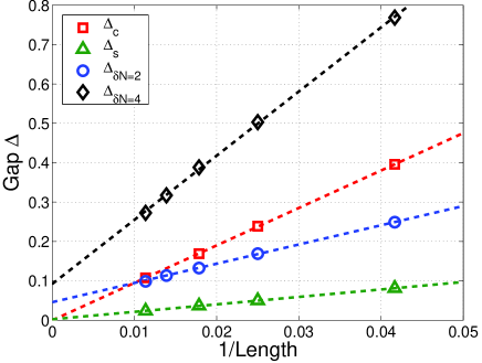
Figure 2: Calculated gaps from DMRG, measured in units of $t_{pd}$, as a function of $1/L$, where $L$ is the number of Cu sites in the system. $\Delta_{c}$ is the charge gap, $\Delta_{s}$ is the spin gap, and $\Delta_{\delta_{N}=2}$ and $\Delta_{\delta_{N}=4}$ are the gaps for transferring one and two holes from one chain to the other (see text). The dashed lines are linear extrapolations.

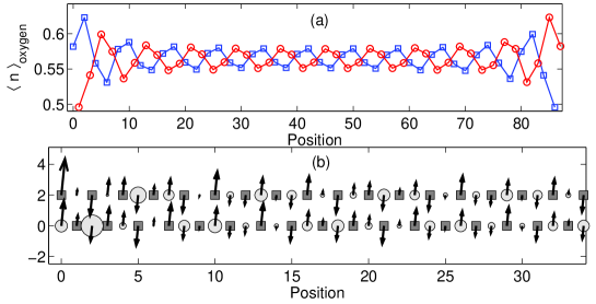
Figure 3: (a) The average hole density on oxygen sites as a function of position. Blue Squares (red circles) mark the upper (lower) chain from the DMRG simulation with $\langle n\rangle=1.25$ holes per Cu site. (b) $\langle S^{z}_{i}\rangle$ as a function of position. Copper sites are marked by squares, and oxygen sites - by circles. The size of the circles represents the average hole density on the oxygen sites (bigger circles mean larger hole density).

The doped zigzag chain cannot be understood as simply as the half filled one. Moreover, it is not entirely clear what doping level leads to superconductivity in Pr-247; counting charges (and assuming that the valence of the Pr ions is $+3$), there are $9/7-2\delta/7$ doped holes per copper site on average, and superconductivity occurs when $\delta\gtrsim 0.3$ (see [YamadaSC1, ]). However, these holes are distributed in an unknown manner between the plane, single chain, and double chain Cu sites. Therefore, we have performed DMRG simulations with a finite doping concentration which we take, somewhat arbitrarily, to be 0.25 “doped holes” per Cu (i.e. the density of holes is taken to be $n=1.25$ per Cu site). The following parameters were used in Eq. (4): $t_{pd}=1$, $\varepsilon=0.5$, and $J_{1}=J_{2}=0.5$ The values for $t_{pd},J_{1}$, and $\varepsilon$ are comparable to values that are commonly used in effective $t-J$ models for the copper-oxide planes in the cuprates. In the simulations described in this section, the direct oxygen-oxygen hopping, $t_{p,p}$, was neglected. (The effect of non-zero $t_{p,p}$ is examined in the next subsection.) Up to $m=2700$ states per block where kept for the longest systems ($L=88$ Cu sites), resulting in an average truncation error of about $10^{-6}$. The energies where extrapolated to zero truncation errors using the standard procedureWhiteExtrap . The convergence of the ground state energy as a function of the number of sweeps improves dramatically when a small perpendicular copper - oxygen term is added to the hopping Hamiltonian (5), with $t_{\perp}=0.01$. We have checked that the physical results are not affected by adding this term.

In Fig. 2 we plot various gaps in the spectrum as a function of $1/L$. $\Delta_{c}=E_{N+2}+E_{N-2}-2E_{N}$ is the charge gap, and $\Delta_{s}=E_{S^{z}=2}-E_{S^{z}=1}$ is the spin gap. We define the spin gap relative to the $S^{z}=1$ state, since the ground state is found to have spin one for the systems considered here. In addition, we have calculated the gap to the state with one or two holes transferred from one chain to the other: $\Delta_{\delta N=2}=E_{\delta N=2}-E_{\delta N=0}$ and $\Delta_{\delta N=4}=E_{\delta N=4}-E_{\delta N=0}$, where $\delta N=N_{2}-N_{1}$ is the difference between the number of holes in the two chains. The direct measurement of $\Delta_{\delta N}$ is possible due to the fact that $N_{1}$ and $N_{2}$ (the numbers of holes on each chain) are separately conserved. In the presence of a small inter-chain hopping term, this conservation law is weakly violated. However, it is still possible to measure $\Delta_{\delta N}$ by applying an inter-chain potential difference $\Delta V$. When $\Delta V=\Delta_{\delta N}$, one hole is transferred from one chain to the other. This transition is smoothed by the inter-chain hopping term, with a width proportional to $t_{\perp}$. For $t_{\perp}=0.01$, we found that this does not considerably limit the accuracy in the determination of $\Delta_{\delta N}$.

The gaps were extrapolated linearly with $1/L$ to the thermodynamic limit ($L\rightarrow\infty$). The charge gap $\Delta_{c}$ extrapolates to very close to zero. The spin gap $\Delta_{s}$ also extrapolates to a very small value, which is indistinguishable from zero to the accuracy of our calculations. However, $\Delta_{\delta N=2}$ and $\Delta_{\delta N=4}$ clearly extrapolate to finite values. The linear extrapolation results are $\Delta_{\delta N=2}(1/L\rightarrow 0)\approx 0.046$, $\Delta_{\delta N=4}(1/L\rightarrow 0)\approx 0.097$.

Let us assume that, as the simulation suggests, $\Delta_{c}=\Delta_{s}=0$. In terms of the classification by the number of gapless bosonic modes, this implies that we must have at least one gapless charge mode and one gapless spin mode. However, since $\Delta_{\delta N}\neq 0$ at least some of the relative spin and charge modes of the two chains are gapped by the inter-chain coupling. The fact that $\Delta_{\delta N=4}\neq 0$ in the thermodynamic limit implies that the relative charge mode is gapped. This is because it involves transferring two holes from one chain to the other, and two holes can be combined to a singlet and therefore carry no spin.

Fig. 3a shows the average hole density on the oxygen sites in a chain of $L=88$ Cu sites. The density profile shows pronounced density oscillations with a period of $\lambda_{c}=4a$ where $a$ is the lattice constant. For the density of holes in the simulation, this corresponds to a wavevector of $4k_{F}$. Fourier transforming the density profile reveals that the $2k_{F}$ component is almost completely absent, which is characteristic of systems with strong repulsion. Note also that the relative charge densities in the two chains appear rigidly locked to each other so that the charge oscillations are strictly staggered, further evidence of the existence of a relative charge gap.

A zigzag chain model similar to Eq. (4) was studied in Ref. [OgataRice, ], and a spin gap was found. However, in that study there where no oxygen sites and it was assumed that $J_{2}<0$ (i.e. antiferromagnetic) and $|J_{2}|>J_{1}$. The ferromagnetic case was studied (in a different context) in Ref. [FMZigzag, ], and their results seem consistent with ours (at least over a certain range of parameters).

In Fig. 3b we show $\langle S_{i}^{z}\rangle$ along with the oxygen site density (represented by the size of the circles) in the same system. A weak Zeeman field $\mathbf{H}=0.01\mathbf{\hat{z}}$ was applied to the first and last Cu sites on the chain in order to select a direction in spin space. The main periodicity in the spin density is $\lambda_{s}=8a$, or $2k_{F}$. Note that a peak in the hole number density is always accompanied by a $\pi$ phase shift in the spin density wave. Some features of the pattern of the charge and spin density can be understood from a strong coupling approach, as discussed in section V A.

IV.2 $t_{pp}\neq 0$ case

So far, we have neglected the oxygen-oxygen hopping $t_{pp}$. This term is expected to be significantly smaller than $t_{pd}$, because of its longer range. Estimates from LDA calculations LDA give $t_{pp}\sim 0.27t_{pd}$YamadaTheory .

As we saw, the DMRG simulation with $t_{pp}=0$ revealed a finite gap to the relative charge mode between the two chains. In such a phase, single particle inter-chain hopping is irrelevantSheltonLadders . Therefore, this phase is expected to be robust over a finite range of $t_{pp}$. However, this argument cannot tell us what is the range of stability. In order to study the effect of a finite $t_{pp}$, we have performed simulations including an oxygen-oxygen hopping term $H_{pp}$. Using the same notation as in Eq. (5), $H_{pp}$ is given by

$$H_{pp}=-t_{pp}\sum_{i,\sigma}\hat{P}\left(p_{x,i,\sigma,1}^{\dagger}p_{x,i+1,\sigma,2}+p_{x,i,\sigma,2}^{\dagger}p_{x,i,\sigma,1}+h.c.\right)\hat{P}$$ (8)

In the presence of this term, the method we used previously to determine whether there is a relative charge gap (based on measuring the energy gap for transferring one hole from one chain to the other) is no longer applicable because now the charges on the two chains are not conserved separately. Consequently, the charge difference cannot be controlled in the calculation. Instead, we used an alternative method to determine in which phase the system is. The local spin and charge densities on each chain where measured and Fourier transformed. We define

$$n_{q} = \frac{1}{\sqrt{L/2}}\sum_{i=1}^{L/2}e^{-iqx_{i}}n_{p_{x},i,1}$$

$$S_{q}^{z} = \frac{1}{\sqrt{L/2}}\sum_{i=1}^{L/2}e^{-iqx_{i}}S_{d,i,1}^{z}$$ (9)

Here $n_{p_{x},i,1}=\sum_{\sigma}p_{x,i,\sigma,1}^{\dagger}p_{x,i,\sigma,1}$, $S_{d,i,1}^{z}=\frac{1}{2}\sum_{\sigma}\sigma d_{i,\sigma,1}^{\dagger}d_{i,\sigma,1}$ and $L$ is the length of the chain (number of Cu sites). Due to the open boundary conditions, $n_{q}$ and $S_{q}^{z}$ show pronounced peaks at certain wavevectors. (These are known as “Friedel-like” oscillationsWhiteFriedel .) These peaks occur at the wavevectors of the gapless spin/charge modes of the system. A 1D version of Luttinger’s theoremAffleck1dLuttinger states that there must be a gapless mode at a certain wavevector, corresponding in our case to $4k_{F}$ of a single chain, where $2k_{F}=\pi n$ ($n$ is the number of holes per Cu site). In addition, there could be other gapless modes at other wavevectors (e.g., charge or spin modes at $2k_{F}$ for each chain, etc.). If there is only a single gapless charge mode, as we found in the case $t_{pp}=0$, then we expect to find gapless modes (and therefore peaks in the Fourier transformed local spin/charge densities of a finite system with open boundary conditions) only at a single wavevector, plus its harmonics. If, on the other hand, the relative charge gap closes and there is more than one gapless charge mode, there is no reason why these modes cannot have different wavevectors (these are the analogues of the two Fermi wavevectors in the non-interacting ladder problem). This way, the phase transition from a phase with a single gapless charge mode to a phase with two gapless modes can be identified.

The results of the DMRG calculations are shown in Fig. 4. No additional peaks appear at new wavevectors and the spin/charge profiles do not change qualitatively until $t_{pp}\sim 0.5-0.6t_{pd}$. This shows that the phase with a single gapless charge mode is robust at least up to $t_{pp}=0.5t_{pd}$, which is higher than the value estimated from band structure calculations for the zigzag CuO chain.

V Analytical results in special limits

V.1 $t_{pd}\rightarrow 0$ limit

We start from a qualitative strong coupling description, in which we assume that $t_{pd}^{2}/\varepsilon\ll J_{1},J_{2}$. As we saw, at half filling the inter-chain coupling $J_{2}$ is frustrated, so the low-energy spectrum is essentially like that of two decoupled chains. A typical snapshot of the spin configuration in this state is depicted in Fig. 5a.

We now consider a lightly hole doped system. Since all the copper sites are occupied, the doped holes reside on oxygen sites. Fig. 5b shows two neighbor holes on opposite chains. Since $J_{1}>0$, every doped hole induces a $\pi$ shift in the phase of the spin density wave around it. The doped hole locally relieves the frustration of the inter-chain ferromagnetic coupling $J_{2}$, causing a net coupling between the spin fluctuations on the two chains. This coupling is proportional to the hole concentration $x$ times $J_{2}$. The hole can move along the chain via a second order process in $t_{pd}$ without disturbing the local spin order. Note that some exchange energy is gained also near the neighbor hole in the opposite chain.

However, if two neighbor holes are in the same chain (as shown in 5c), the situation is different. Now we cannot satisfy the $J_{2}$ terms near both holes, and the inter-chain coupling is partially frustrated. Therefore, the lowest energy states will be ones in which the holes appear in alternating order in the two chains. The holes are free to move so as to reduce their zero point kinetic energy, as long as they do not pass each other.

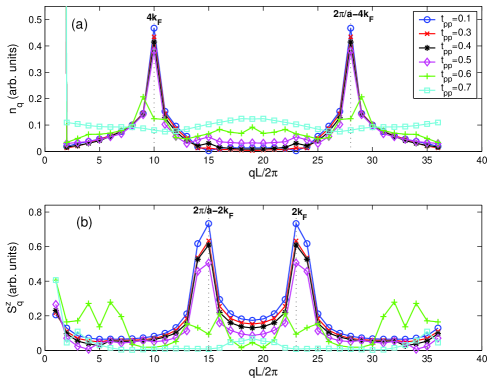
Figure 4: (Color online.) Fourier transforms of the charge (a) and spin (b) profiles (defined in Eq. (9)) calculated by DMRG in a system of length $L=72$ Cu sites. Various values of $t_{pp}$ (Eq. (8)) were used. ($t_{pp}$ is measured in units of $t_{pd}$.) Both profiles change qualitatively and new peaks appear between $t_{pp}=0.5t_{pd}$ and $0.6t_{pd}$, which signals a phase transition to a phase with two independent gapless charge modes.

The qualitative picture in the small $t_{pd}$ limit can explain some of the features in Fig. 3b. As mentioned previously, the peaks in the charge density on the O sites are accompanied by $\pi$ phase shifts in the spin density wave on the Cu sites, which can be understood as coming from the antiferromagnetic coupling between neighboring Cu and O spins. The fact that the hole density oscillations are $\pi$ phase shifted between the two chains, is reminiscent of the alternating order between the chains described above. Moreover, the spin on the O site with maximum local density is always parallel to the spin of the nearest Cu on the opposite chain, due to the ferromagnetic coupling between them. The DMRG picture is therefore qualitatively very similar to Fig. 5 even though $t_{pd}$ is not small.

In fact, we suspect that the present analysis is qualitatively correct for small enough $x$ independent of the magnitude of $t_{pd}$. For a single hole in an antiferromagnetic chain, a $\pi$ phase shift in the antiferromagnetic correlations appears to be generic. Beyond that, the energy which favors alternating holes on the two chains is purely geometric in origin, and so only requires that the holes be sufficiently dilute.

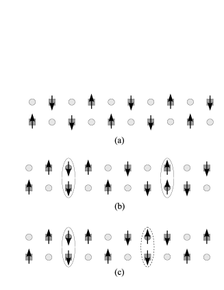
Figure 5: Typical pattern of the spin correlations in various situations. Copper (oxygen) sites are shown as square (circles). (a) The undoped chain. The intra-chain interaction is antiferromagnetic, while the ferromagnetic inter-chain interaction is frustrated. (b) Two doped holes, one in each chain. Note that the phase of the spin fluctuation shifts by $\pi$ around the doped holes. The spin of each doped holes is parallel to the spin of the nearest copper site in the opposite chain, which gains some ferromagnetic interchain exchange energy. (c) Two doped holes in the same chain. This is similar to (b), except that now the inter-chain ferromagnetic exchange energy of the hole on the right is lost. Putting two neighboring doped holes in the same chain is less favorable energetically.

V.2 RG and Bosonization treatment

Another limit of the zigzag chain model (4) that can be treated analytically is the weak inter-chain coupling limit ($|J_{2}|\ll J_{1},t$). In this limit, only the low-energy degrees of freedom of the decoupled chains are affected by the inter-chain coupling. These degrees of freedom can be described as two Luttinger liquids. The inter-chain coupling can then be treated using perturbative RG. The nature of the strong-coupling fixed point can be understood using abelian bosonization. This is a standard procedureBalentsFisher ; CongjunFradkin .

As we will see, in the weak inter-chain coupling limit a spin gap is predicted, in contradiction to DMRG results of section IV.1. The discrepancy can be explained by the fact that the inter-chain coupling is not small. Rather, we will use bosonization to parameterize an effective low energy model which is consistent with the numerical results. This model is then used to calculate low-energy susceptibilities of the system.

The Hamiltonian is written as

$$H=H_{LL}+H_{int}$$ (10)

Here $H_{LL}$ is a Luttinger liquid Hamiltonian that describes the low energy degrees of freedom of each chain, and $H_{int}$ is the inter-chain coupling Hamiltonian,

$$H_{LL}=H_{0,s}+H_{0,c}$$ (11)

where $H_{0,s}$ and $H_{0,c}$ are bosonic Hamiltonians for the spin and charge modes of each chain:

$$H_{0,s}=\frac{u_{s}}{2}\sum_{i=1,2}\int dx\left[K_{s}\left(\partial_{x}\theta_{i,s}\right)^{2}+\frac{1}{K_{s}}\left(\partial_{x}\varphi_{i,s}\right)^{2}\right]$$ (12)

$$H_{0,c}=\frac{u_{c}}{2}\sum_{i=1,2}\int dx\left[K_{c}\left(\partial_{x}\theta_{i,c}\right)^{2}+\frac{1}{K_{c}}\left(\partial_{x}\varphi_{i,c}\right)^{2}\right]$$

and $i=1,2$ is the chain index. SU$\left(2\right)$ symmetry gives the constraint $K_{s}=1$, while $K_{c}<1$ depends on the details of the intra-chain microscopic interactions. Here $\phi$ and $\theta$ represent dual fields, i.e. $[\partial_{x}\theta_{a}(x),\phi_{b}(x^{\prime})]=i\delta_{a,b}\delta(x-x^{\prime})$, and are related to the density and current operators, e.g. $\rho_{i}=\sqrt{2/\pi}\partial_{x}\phi_{i,c}$ and $j_{i}=u_{c}\sqrt{2/\pi}\partial_{x}\theta_{i,c}$ where $\rho_{i}$ and $j_{i}$ are, respectively, the electron density and current density on chain $i$. At half filling, the charge sector will also have a non-linear term $g_{u}\cos(\sqrt{8\pi}\varphi_{c,i})$, which corresponds to $4k_{F}$ umklapp scattering. The spin sector should include marginally irrelevant operators, which we have not written here.

Next, we consider the interaction term between the two chains. This term is most conveniently written in terms of the corresponding fermionic degree of freedom, $\psi_{i,\sigma}$, with $i=1,2$ for the two chains, which is in turn written in terms of the right and left moving fermions, $\psi_{i,\sigma}\sim e^{ik_{F}x}\psi_{i,R,\sigma}+e^{-ik_{F}x}\psi_{i,L,\sigma}$, where $2k_{F}=\pi n$ is the Fermi wavevector ($n$ is the total density of holes). Taking a naive continuum limit of the $J_{2}$ term in (6), we get:

$$H_{int} = J_{2}a\int dx{\LARGE\{}\ \mathbf{S}_{1}\left(x\right)\cdot\mathbf{S}_{2}\left(x\right)+\mathbf{S}_{1}\left(x\right)\cdot\mathbf{S}_{2}\left(x+a\right)$$ (13)

$$- \frac{1}{4}\left[n_{1}\left(x\right)n_{2}\left(x\right)+n_{1}\left(x\right)n_{2}\left(x+a\right)\right]{\LARGE\}}$$

Here $\mathbf{S}_{i}\left(x\right)=\psi_{i}^{\dagger}\left(x\right)\vec{\sigma}\psi_{i}\left(x\right)$, $n_{i}\left(x\right)=\psi_{i}^{\dagger}\left(x\right)\psi_{i}\left(x\right)$, and $a$ is the lattice constant. This form satisfies the requirement that the Hamiltonian is symmetric with respect to $\mathbf{S}_{1}\left(x\right)\rightarrow\mathbf{S}_{2}\left(x\right)$, $\mathbf{S}_{1}\left(x\right)\rightarrow\mathbf{S}_{2}\left(x+a\right)$ and similarly for the $n_{i}$’s, which corresponds to a reflection that interchanges the two chains, followed by a translation by one Cu-O distance.

In bosonized form, the most relevant part of (13) is written as:

$$H_{int} = -\frac{\sin(\frac{\delta a}{2})}{(\pi a)^{2}}\int dx\sin\left(\sqrt{4\pi}\varphi_{-,c}-\frac{\delta a}{2}\right)$$ (14)

$$\times\left[g_{1}\hat{\mathcal{O}}_{s1}+g_{2}\hat{\mathcal{O}}_{s2}\right]$$

Here $\hat{\mathcal{O}}_{s1}\equiv\left[\cos\left(\sqrt{4\pi}\varphi_{-,s}\right)+\cos\left(\sqrt{4\pi}\theta_{-,s}\right)\right]$ and $\hat{\mathcal{O}}_{s2}\equiv\left[\cos\left(\sqrt{4\pi}\varphi_{-,s}\right)+\cos\left(\sqrt{4\pi}\varphi_{+,s}\right)\right]$ where $\varphi_{\pm,c}=\left(\varphi_{1,c}\pm\varphi_{2,c}\right)/\sqrt{2}$ are the even/odd charge modes of the two chains, and similarly for $\varphi_{\pm,s}$ and $\theta_{\pm,s}$. We have defined $\delta=\pi(n-\frac{1}{a})$, where $n$ is the density of holes per unit length. ($\delta$ is a wavevector whose length is proportional to the amount of doping away from half filling.) At half filling, additional umklapp terms appear. $g_{1}$ and $g_{2}$ are dimensionless coupling constants, whose bare values at the initial scale are: $g_{1}=-g_{2}=\frac{J_{2}a}{2}$. Under RG, $g_{1}$ and $g_{2}$ will flow, and need not remain equal in magnitude. However, additional couplings are prevented as long as the exact SU$(2)$ spin-rotational symmetry is respected. Specifically, there are three distinct cosines of spin fields, but only two independent coupling constants.

Note that the inter-chain coupling (13) vanishes in the limit $\delta\rightarrow 0$, i.e. at half filling. This is due to the frustration of the inter-chain coupling in that limit. (See section III. ) Then marginal operators need to be considered. These produce an extremely small gap in the spectrum, especially in the $J_{2}<0$ case ItoiZigzag , so the system can be considered as essentially gapless at half fillingWhiteZigzag ; ItoiZigzag .

Away from half filling, both the $g_{1}$ and $g_{2}$ terms in (14) are relevant, and produce a gap in the spectrum. They both have the same scaling dimension of $1+K_{+,c}<2$ (assuming that $K_{\pm,s}=1$). The system flows to a strong coupling fixed point at which the $\varphi_{-,c}$, $\varphi_{+,s}$ and $\theta_{-,s}$ fields are pinned. Then the only gapless mode is the total charge mode, and the system is in a C₁S₀ phase, similar to the generic situation in the Hubbard ladderBalentsFisher .

However, the DMRG result indicates that while there is a substantial gap in the relative charge mode, the gap in the total spin sector is either zero or very small (see Fig. 2). This discrepancy is likely to be caused by less relevant (sub-leading) operators, not included in Eq. (14), whose bare coefficients are of order unity (since we are not initially at weak coupling). The neglect of these operators in the initial stages of the RG transformation is a quantitatively unreliable approximation. Taking the DMRG result into account, we hypothesize that the effective value of $g_{2}$ at the fixed point is close to 0 (since non-zero $g_{2}$ is what induces a full spin-gap). If this is true, then over a broad intermediate range of energies, the system is governed by the unstable fixed point with $g_{2}=0$ and non-zero $g_{1}$.

We would like to stress that the smallness of the spin gap is not a result of fine tuning, but rather appears (from the numerics) to be a ubiquitous property of the model. (The same result is obtained over a range of different parameters and doping levels.) In contrast, if the inter-chain coupling $J_{2}$ is artificially turned to be antiferromagnetic, a spin gap appears in the numerical simulation. Therefore the small spin gap seems to be a feature of the ferromagnetic $J_{2}$ case.

Note that the phase with $g_{1}\neq 0$, $g_{2}=0$ is unusual, because neither the field $\varphi_{-,s}$ nor its dual $\theta_{-,s}$ can be pinned (since $\hat{\mathcal{O}}_{s1}$ contains the cosine terms containing both fields with equal magnitude). The properties of this phase, which follow closely from an earlier analysis of the Heisenberg ladder by Shelton, Nersessyan and TsvelikSheltonTsvelik , are explored in appendix A. The main conclusion is that essentially “half” of the relative spin mode is gapped, and the other half is gapless. Therefore we denote this phase as C₁S${}_{\frac{3}{2}}$.

V.3 Physical susceptibilities

Given that the system is in a C₁S${}_{\frac{3}{2}}$ phase, the physical susceptibilities can be calculated in a similar way to that described in [SheltonTsvelik, ], with addition of the charge modes. For an example of such a calculation, see appendix A. The leading temperature dependence of these susceptibilities depends only on the total charge Luttinger parameter $K_{+,c}$. The superconducting susceptibility is

$$\chi_{SC}\sim T^{\frac{1}{2K_{+,c}}-\frac{5}{4}}$$ (15)

for both singlet and triplet pairing, which gives that the superconducting susceptibility is divergent for $K_{+,c}>0.4$ (i.e. even for strongly repulsive interactions).

Other susceptibilities are $2k_{F}$ SDW and CDW, with

$$\chi_{SDW,2k_{F}}\sim\chi_{CDW,2k_{F}}\sim T^{\frac{K_{+,c}}{2}-\frac{5}{4}}$$ (16)

and $4k_{F}$ CDW:

$$\chi_{CDW,4k_{F}}\sim T^{2K_{+,c}-2}$$ (17)

The superconducting susceptibility is the most divergent one for $K_{+,c}>1$.

Assuming that the relative charge mode $\varphi_{-,c}$ is gapped, it is possible to extract $K_{+,c}$ from the density profile in the DMRG simulation (see Fig. 3). The density profile is expected to behave as $\langle n_{i}\rangle\sim\cos(4k_{F}x_{i})/[L\sin(\pi x_{i}/L)]^{K_{+,c}}$, which is essentially the square root of the $4k_{F}$ part of the density-density correlation function WhiteFriedel . The amplitude of the $4k_{F}$ CDW near the middle of the chain, $A_{x_{i}=L/2}$, thus decays as $L^{-K_{+,c}}$. Fitting $A_{x_{i}=L/2}$ of chains with different lengths to this expression, we obtain $K_{+,c}=0.6\pm 0.05$.

Since NQR measures of the spin-lattice relaxation rate have been done on superconducting Pr-247, it is interesting to extract the temperature dependence of this quantity from the theory. Assuming that the main relaxation mechanism is the coupling of the nuclear spins to fluctuations of the local magnetic field due to electronic spins, $1/T_{1}$ is given byScalapinoNMR :

$$\frac{1}{T_{1}}=\frac{1}{2N}\sum_{q\alpha}\left|A_{\alpha}\left(q\right)\right|^{2}S^{\alpha\alpha}\left(q,\omega_{R}\right)$$ (18)

where $A_{\alpha}\left(q\right)$ is the form factor of the hyperfine Hamiltonian, $\omega_{R}$ is the nuclear spin resonance frequency, and $S^{\alpha\alpha}\left(q,\omega_{R}\right)$ is the electronic spin structure factor. $\omega_{R}$ is typically smaller than any other energy scale in the problem, so we will assume $\omega_{R}=0$.

The spin structure factor in the C₁S${}_{\frac{3}{2}}$ is expected to be of the form:

$$S^{\alpha\alpha}\left(q,\omega=0\right)\sim A\ln q+Bq^{\frac{K_{+,c}}{2}-\frac{5}{4}}$$ (19)

where $A$ and $B$ are constants. The two terms here are the two main contributions to $S^{\alpha\alpha}(q,\omega=0)$ which come the vicinity of the points $q=0,2k_{F}$. Integrating (19) over $q$, we get the dominant temperature dependence of the spin-lattice relaxation rate:

$$\frac{1}{T_{1}}\sim AT\ln T+BT^{\frac{K_{+,c}}{2}-\frac{1}{4}}$$ (20)

NQR measurementsYamadaNQR ; SasakiNQRarchive show that $T_{1}^{-1}$ behaves as a power law of temperature, with different exponents above and below $T_{c}$. The fact that a power law is seen above $T_{c}$ is a clear evidence for the absence of a spin gap, and is consistent with a C₁S${}_{\frac{3}{2}}$ phase. According to the measurement, $\frac{1}{T_{1}}\propto T^{0.5}$ above $T_{c}$. Comparing this behavior to (20), we see that it corresponds to $K_{+,c}\simeq 1.5$. This is consistent with dominant superconducting correlations.

The value of $K_{+,c}$ extracted from the NQR data is substantially larger than the one extracted from our DMRG calculation. Clearly, this is a significant discrepancy. However, it is well known that $K_{+,c}$ is a non-universal exponent, and in this case it depends strongly on microscopic details of the problem. Since the detailed aspects of the microscopic model are certainly not “realistic,” we do not feel that any microscopic calculation can be expected to predict the experimental value of $K_{+,c}$ reliably. A better strategy is thus to extract $K_{+,c}$ directly from experiments. As we saw, in the superconducting sample this yields a value of $K_{+,c}$ that corresponds to dominant superconducting fluctuations.

The NQR measurement was done on with a sample with an oxygen content $\delta=0.5$ which is close to the optimal value for superconductivity. We are not aware of any similar NQR data on samples with a different O content and $T_{c}$. Were such data obtained, we would predict a smaller power should govern the $T$ dependence of $1/T_{1}(T)$, corresponding to a lower $K_{+,c}$.

VI Conclusions

To summarize, we have considered the possibility of zigzag chain-driven superconductivity in Pr₂Ba₄Cu₇O_15-δ. Assuming that the chains are weakly coupled, this implies that the single zigzag chain must have a large superconducting susceptibility. This, in conjunction with the fact that Cu NQR experiments do not show any spin gap above $T_{c}$, raises the possibility that the zigzag chain is in a phase in which some, but not all, of the modes of the two-component electron gas are gapped. We have shown evidence for such a phase using a microscopic copper-oxygen model for the zigzag chain.

The gapping of some of the relative spin and charge modes enhances superconducting (as well as other) fluctuations at low temperatures. The pairing operator is composed of one hole from each chain with zero center of mass momentum. Since there is no spin gap, triplet and singlet superconducting fluctuations are equally enhanced.

Acknowledgements. We thank S. Sasaki and Y. Yamada for discussions and for sharing their data with us before publication. S. Moukouri and S. R. White are acknowledged for their help with setting up the DMRG code. Discussions with E. Altman, O. Vafek and C. Wu are gratefully acknowledged. We thank A. M. Tsvelik for critically reading this manuscript. E.B. also thanks the hospitality of the Weizmann institute, were part of this work was done. This work was supported in part by NSF grant # DMR -551196 at Stanford.

Appendix A The C₁S${}_{\frac{3}{2}}$ phase

We would like to describe a phase of the two-component electron gas with a gap in the relative spin and charge sectors, but no gap in the total spin and charge sectors. This is the phase that seems to emerge from the DMRG results. (See Fig. 2.) Starting from the Hamiltonian $H=H_{LL}+H_{int}$, where $H_{LL}$ is a Luttinger liquid intra-chain Hamiltonian (11) and $H_{int}$ is the most relevant part of a generic SU$\left(2\right)$ invariant inter-chain interaction (Eq. 14), we see that in order for the spin gap to vanish we must have $g_{2}=0$ in (14)). The remaining term is then proportional to $\hat{\mathcal{O}}_{s1}=\cos\left(\sqrt{4\pi}\varphi_{-,s}\right)+\cos\left(\sqrt{4\pi}\theta_{-,s}\right)$. The total scaling dimension of this term with respect to the Luttinger liquid fixed point is $1-K_{-,c}$, with $K_{-,c}<1$, so it will grow under an RG transformation. At some scale, $g_{1}$ becomes of the order of unity, and we can replace $\sin\left(\sqrt{4\pi}\varphi_{-,c}\right)$ and $\cos\left(\sqrt{4\pi}\varphi_{-,c}\right)$ by their mean value (since the field $\varphi_{-,c}$ will be pinned to the minimum of the potential). However, since the interaction contains the cosines of the conjugate fields $\varphi_{-,s}$ and $\theta_{-,s}$ with an equal weights, both fields fluctuate strongly at the fixed point, and neither is pinned. We are faced with the problem of how to describe the low-energy properties of the resulting phase.

A remarkably elegant solution for this problem is given in a paper by Shelton et al [SheltonTsvelik, ]. They considered the problem of two weakly coupled spin $\frac{1}{2}$ chains, but the results are readily generalized to our case by neglecting the fluctuations in the $\varphi_{-,c}$ field, replacing it by its mean value. The Hamiltonian (10) can then be solved by re-fermionizing of the fields $\varphi_{\pm,s}$. We introduce two Dirac fermions, $\psi$ and $\chi$, as follows:

$$\psi_{R,L} = \frac{1}{\sqrt{2\pi a}}e^{i\sqrt{\pi}\left(\theta_{+,s}\pm\varphi_{+,s}\right)}$$

$$\chi_{R,L} = \frac{1}{\sqrt{2\pi a}}e^{i\sqrt{\pi}\left(\theta_{-,s}\pm\varphi_{-,s}\right)}$$ (21)

where $R$ and $L$ denote right or left moving fields. The Hamiltonian for $\psi$ is then just a free Dirac Hamiltonian:

$$H_{+}=u_{s}\int dx\left(\psi_{R}^{\dagger}\frac{1}{i}\frac{d}{dx}\psi_{R}-\psi_{L}^{\dagger}\frac{1}{i}\frac{d}{dx}\psi_{L}\right)$$ (22)

The interaction Hamiltonian $H_{int}$ (13) becomes quadratic in $\chi$, giving

$$H_{-} = u_{s}\int dx\left(\chi_{R}^{\dagger}\frac{1}{i}\frac{d}{dx}\chi_{R}-\chi_{L}^{\dagger}\frac{1}{i}\frac{d}{dx}\chi_{L}\right)$$ (23)

$$+ \frac{iM}{4}\int dx\left(\chi_{R}^{\dagger}\chi_{L}+\chi_{L}^{\dagger}\chi_{R}^{\dagger}-\text{H.c.}\right)$$

Here $M$ depends on $g_{1}$ and the average of the $\varphi_{-,c}$ part in (13). (23) is most conveniently diagonalized by writing $\chi$ in terms of two Majorana fermions. Adopting the notation of [SheltonTsvelik, ], we write

$$\xi_{\nu} = \frac{\chi_{\nu}+\chi_{\nu}^{\dagger}}{\sqrt{2}}$$

$$\rho_{\nu} = \frac{\chi_{\nu}-\chi_{\nu}^{\dagger}}{i\sqrt{2}}$$ (24)

with $\nu=R,L$. Plugging this into (23), we get:

$$H_{-}=H_{0}\left[\xi\right]+H_{M}\left[\rho\right]$$ (25)

$$H_{0}\left[\xi\right]=\frac{u_{s}}{2}\int dx\left(\xi_{R}\frac{1}{i}\frac{d}{dx}\xi_{R}-\xi_{L}\frac{1}{i}\frac{d}{dx}\xi_{L}\right)$$ (26)

$$H_{M}\left[\rho\right] = \frac{u_{s}}{2}\int dx\left(\rho_{R}\frac{1}{i}\frac{d}{dx}\rho_{R}-\rho_{L}\frac{1}{i}\frac{d}{dx}\rho_{L}\right)$$ (27)

$$+\frac{iM}{2}\int dx\left(\rho_{R}\rho_{L}-\rho_{L}\rho_{R}\right)$$

The field $\xi$ is thus massless, while $\rho$ is massive, with a mass $M$. In that sense, “half” of the field $\varphi_{-,s}$ is gapped. The total spin sector, on the other hand, is completely massless. We therefore denote this phase as a C₁S${}_{\frac{3}{2}}$ phase.

Setting $g_{2}\neq 0$ in (13) will gap out also the total spin mode, giving a C₁S₀ phase. Moreover, adding less relevant inter- or intra-chain operators to (13) would generate the $g_{2}$ term, even if it is not present in the bare Hamiltonian. However, the DMRG calculation presented in section IV.1 indicates that the spin gap $\Delta_{s}$ is much smaller than $\Delta_{\delta N}$, the gap to transferring one hole from one chain to the other, which is related to a gap in the relative spin/charge modes. Therefore, at intermediate energies (or temperatures) between $\Delta_{s}$ and $\Delta_{\delta N}$, the physics is expected to be dominated by the unstable C₁S${}_{\frac{3}{2}}$ fixed point.

Next, let us find the long-distance behavior of the correlation functions of physical operators in the C₁S${}_{\frac{3}{2}}$ phase. For concreteness, we will focus on the pair field operator $\Delta_{SC}=\psi_{1R,\uparrow}\psi_{2L,\downarrow}$. This operator creates a pair of holes in the two chains with opposite momenta and spins. In bosonized form, this operator becomes

$$\Delta_{SC}\sim e^{i\sqrt{\pi}\left(\theta_{+c}+\theta_{-,s}+\varphi_{-,c}+\varphi_{+,s}\right)}$$ (28)

$\theta_{+c}$ is a free bosonic field, whose long-range correlations are $\left\langle e^{i\sqrt{\pi}\theta_{+,c}\left(x\right)}e^{i\sqrt{\pi}\theta_{+,c}\left(0\right)}\right\rangle\sim x^{-\frac{1}{2K_{+,c}}}$. Similarly, $\left\langle e^{i\sqrt{\pi}\varphi_{+,s}\left(x\right)}e^{i\sqrt{\pi}\varphi_{+,s}\left(0\right)}\right\rangle\sim x^{-\frac{1}{2}}$, since $\varphi_{+,s}$ is a free field with $K_{+,s}=1$, as dictated by the SU$\left(2\right)$ symmetry. This correlation function is expected to have logarithmic corrections due to marginal operators, which we have neglected. The $\varphi_{-,c}$ field is massive, so at long distances we can replace $e^{i\sqrt{\pi}\varphi_{-,c}}$ by its expectation value. The treatment of $e^{i\sqrt{\pi}\theta_{-,s}}$ is more subtle, since as we have mentioned, this field is “half gapped” in the C₁S${}_{\frac{3}{2}}$ phase. It is nevertheless possible to calculate its correlations, following a method used in [SheltonTsvelik, ]. We describe this method briefly here. The relative spin sector, which is described as two independent Majorana theories, can be further mapped onto two 2d Ising models. Since one of the Majorana fields is massless and the other is massive, one of the corresponding Ising fields is at criticality and the other is away from criticality. It can be shown that the four operators $\sin\left(\sqrt{\pi}\theta_{-,s}\right)$, $\cos\left(\sqrt{\pi}\theta_{-,s}\right)$, $\sin\left(\sqrt{\pi}\varphi_{-,s}\right)$, $\cos\left(\sqrt{\pi}\varphi_{-,s}\right)$ have the following correspondance to the order and disorder operators of the two Ising modelsSheltonTsvelik ; ShankarBosonization :

$$\cos\sqrt{\pi}\varphi_{-,s} = \mu_{1}\mu_{2}\text{, \ \ \ }\sin\sqrt{\pi}\varphi_{-,s}=\sigma_{1}\sigma_{2}$$

$$\cos\sqrt{\pi}\theta_{-,s} = \mu_{1}\sigma_{2}\text{, \ \ \ }\sin\sqrt{\pi}\theta_{-,s}=\sigma_{1}\mu_{2}$$ (29)

Here $\sigma_{1}$, $\mu_{1}$, $\sigma_{2}$, $\mu_{2}$ are the order/disorder operators of the two Ising models labelled 1 and 2. Note that the scaling dimension of all the operators in the left hand side of (29) at criticality is $\frac{1}{4}$, which is consistent with the fact that the dimension of the Ising operators at criticality is $\frac{1}{8}$. Carrying out the correspondence to the Ising model carefully, one finds that the Ising model labelled by 1 is in its disordered phase, so $\left\langle\mu_{1}\right\rangle\neq 0$, $\left\langle\sigma_{1}\right\rangle=0$. The other Ising model labelled by 2 is critical, and therefore $\left\langle\sigma_{2}\left(x\right)\sigma_{2}\left(0\right)\right\rangle\sim x^{-\frac{1}{4}}$, and similarly for $\mu_{2}$. Thus at long distances, $\left\langle e^{i\sqrt{\pi}\theta_{-,s}\left(x\right)}e^{i\sqrt{\pi}\theta_{-,s}\left(0\right)}\right\rangle\sim x^{-\frac{1}{4}}$. The exponent of this correlation function is just half of the exponent that one gets for a free $\theta_{-,s}$ field. This can be understood as a consequence of the fact that “half” of the $-,s$ mode is gapped. Therefore, correlation function of $\Delta_{SC}$ behaves as

$$\left\langle\Delta_{SC}^{\dagger}\left(x\right)\Delta_{SC}\left(0\right)\right\rangle\sim\frac{1}{x^{\frac{1}{2K_{+,c}}+\frac{3}{4}}}$$ (30)

which gives a superconducting susceptibility that behaves as $\chi_{SC}\left(T\right)\sim T^{\frac{1}{2K_{+,c}}-\frac{5}{4}}$. The correlation functions of other physical operators (CDW, SDW etc.) can be calculated in a similar manner.

It is interesting to note that the Hamiltonian (14) with $g_{2}=0$ is equivalent to the integrable super-symmetric super-Sine-Gordon modelTsvelikSSGmodel .

References

- (1) For a review, see E. W. Carlson, D. Orgad, S. A. Kivelson, and V. J. Emery, Phys. Rev. B 62, 3422 (2000).
- (2) M. Matsukawa, Y. Yamada, M. Chiba, H. Ogasawara, T. Shibata, A. Matsushita, Y. Takano, Physica C 411 (2004) 101.
- (3) Y. Yamada, A. Matsushita, Physica C 426 (2005) 213.
- (4) S. Watanabe, Y. Yamada and S. Sasaki, Physica C 426 (2005), 473.
- (5) S. Sasaki, S. Watanabeb and Y. Yamadac, Journal of Magnetism and Magnetic Materials 310, 696-697 (2007); S. Sasaki, S. Watanabe, Y. Yamada, F. Ishikawa, K. Fukuda and S. Sekiya, unpublished (to be submitted to Phys. Rev. Lett.).
- (6) S. Horii, U. Mizutani, H. Ikuta, Y. Yamada, J. H. Ye, A. Matsushita, N. E. Hussey, H. Takagi and I. Hirabayashi, Phys. Rev. B 61, 6327 (2000).
- (7) M. N. McBrien, N. E. Hussey, P. J. Meeson, S. Horii and H. Ikuta, J. Phys. Soc. Jpn. 71, 701 (2002).
- (8) N. E. Hussey, M. N. McBrien, L. Balicas, J. S. Brooks, S. Horii, and H. Ikuta, Phys. Rev. Lett. 89, 086601 (2002).
- (9) K. Sano, Y. Ōno and Y. Yamada, J. Phys. Soc. Jpn 74, 2885 (2005).
- (10) K. Okunishi, Phys. Rev. B75, 174514 (2007).
- (11) T. Nakano, K. Kuroki and S. Onari, cond-mat/0701160.
- (12) S. Gopalan, T.M. Rice and M. Sigrist, Phys. Rev. B49, 8901 (1994).
- (13) L. Balents and M. P. A. Fisher , Phys. Rev. B53, 12133 (1996).
- (14) C. Wu, W. V. Liu and E. Fradkin, Phys. Rev. B68, 115104 (2003)
- (15) H. J. Schulz, Phys. Rev. B59, R2471(1999).
- (16) A model of two Luttinger liquids coupled by Hubbard and exchange interactions (but not by direct hopping) was studied in: D. G. Shelton and A. M. Tsvelik, Phys. Rev. B53, 14036 (1996).
- (17) M. Ogata, M. U. Luchini and T. M. Rice, Phys. Rev. B44, 12083(R) (1991).
- (18) S. Nishimoto, T. Shirakawa and Y. Ohta, Journal of Magnetism and Magnetic Materials 310, 669–671 (2007).
- (19) S. R. White and I. Affleck, Phys. Rev. B 54, 9862 (1996).
- (20) C. Itoi and S. Qin, Phys. Rev. B 63, 224423 (2001).
- (21) A. A. Nersesyan, A. O. Gogolin, and F. H. L. Eßler, Phys. Rev. Lett. 81, 910 (1998).
- (22) J. Bonča, J. E. Gubernatis, M. Guerrero, E. Jeckelmann and S. R. White, Phys. Rev. B 61, 3251 (2000).
- (23) C. Ambrosch-Draxl, P. Blaha and K. Schwarz, Phys. Rev. B 44, 5141 (1991).
- (24) S. R. White, I. Affleck and D. J. Scalapino, Phys. Rev. B65, 165122 (2002).
- (25) M. Yamanaka, M. Oshikawa and I. Affleck, Phys. Rev. Lett. 79, 1110 - 1113 (1997).
- (26) D. G. Shelton, A. A. Nersesyan and A. M. Tsvelik, Phys. Rev. B53, 8521 (1996).
- (27) N. Bulut, D. W. Hone, D.J. Scalapino and N. E. Bickers, Phys. Rev. B41, 1797 (1990).
- (28) R. Shankar, ”Bosonization: How to make it work for you in Condensed Matter Physics”, BCSPIN School at Kathmandu (1991), in Current Topics in Condensed Matter and Particle Physics, edited by J. Pati, Q. Shafi, and Yu Lu (World Scientific, Singapore, 1993).
- (29) A. M. Tsvelik, Sov. J. Nucl. Phys. 47, 172 (1988).